Observations and modeling of the elasto–gravity signals preceding ...

This is the author’s version of the work. It is posted here by permission of the AAAS for personal use, not for redistribution. The definitive version was published in Science Journal, 358, 1164-1168, doi :10.1126/science.aao0746, 2017.

Observations and modeling of the elasto–gravity signals preceding direct seismic waves Martin Vallée,1∗ Jean Paul Ampuero,2 Kévin Juhel,1 Pascal Bernard,1 Jean-Paul Montagner,1 Matteo Barsuglia3 1

Institut de Physique du Globe de Paris, Sorbonne Paris Cité, Université Paris Diderot, CNRS, France

2

Seismological Laboratory, California Institute of Technology, USA 3 AstroParticule et Cosmologie, Université Paris Diderot,

CNRS/IN2P3, CEA/Irfu, Observatoire de Paris, Sorbonne Paris Cité, France ∗

To whom correspondence should be addressed; E-mail: [email protected]

After an earthquake, the earliest deformation signals are not expected to be carried by the fastest (P) elastic waves, but by the speed–of–light changes of the gravitational field. However, these perturbations are weak and, so far, their detection has not been accurate enough to fully understand their origins and to use them for a highly valuable rapid estimate of the earthquake magnitude. We show that gravity perturbations are particularly well observed with broadband seismometers at distances between 1000 and 2000 kilometers from the source of the 2011, Mw=9.1, Tohoku earthquake. We can accurately model them by a new formalism, taking into account both the gravity changes and the gravity–induced motion. These prompt elasto–gravity signals open the window for minute timescale magnitude determination for great earthquakes. 1

One sentence summary : Earthquakes generate quantifiable signals before direct elastic waves, offering a new early way for magnitude determination.

Earthquakes involve the displacement of large amounts of mass, which modifies the gravity field. This effect is not restricted to a permanent gravity change due to the final mass redistribution (e.g. 1–3), but is also induced by the transient density perturbations carried by seismic waves. During the wave propagation, an observer feels attracted by the compressed parts of the medium and repelled by its dilated parts, with a global net effect depending on the earthquake mechanism. The gravity perturbations are transmitted at the speed of light (3.105 km/s), far faster than the first–arriving (P) elastic waves that travel at 6 to 10 km/s in the crust and upper mantle. Additionnally, at distances close from a large earthquake, the information provided by elastic waves is complex to convert in terms of event magnitude, even when the area is densely instrumented by seismometers. In the case of the 2011, Mw = 9.1, Tohoku earthquake the near–real–time magnitude provided by the authoritative Japan Meteorological Agency (4) was 7.9, and was corrected only 3 hours later to 8.8 (5). This underestimation is due to the fact that real–time local magnitudes are generally derived from instrumental peak amplitudes, which are poorly correlated with moment magnitude when the earthquake is large. Detection of the gravity perturbations would provide a much faster method for identifying fault ruptures. The theoretical relations between the elastic and gravitational fields are well known (e.g. 6), and analytical computations predicted the expected gravity change ∆gP before the arrival of the P waves, in full–space (7) and half–space (8) models. The amplitude of ∆gP increases with increasing elastic deformation of the medium and this growth is faster when the earthquake seismic moment rises quickly. Therefore the large magnitude and short duration earthquakes offer the best observation potential. As shown by (7) and (9), the optimal distances for detecting ∆gP are not the closest ones from the earthquake. As long as the earthquake is in its accel2

erating phase, with seismic moment growing faster than quadratically with time, the gravity acceleration expected just before the arrival of the hypocentral P–wave grows with the distance to the earthquake. For a very large earthquake of magnitude 9 for which the accelerating phase lasts on the order of 100 s, the gravity signal is expected to increase with distance at least up to 800 km from the earthquake. This effect stems from the fact that an earthquake source is not instantaneous, and from the increasing duration of the pre–P observation window with distance. It is, however, not the only reason why close distances can be unfavorable to observe the early gravity signals with seismometers or gravimeters coupled to the ground. A previously overlooked phenomenon arises from ground accelerations themselves induced by the gravity changes, which tend to reduce the observability of the signal at early times. The Tohoku earthquake in Japan (11 March 2011, Mw magnitude 9.1) was a suitable event to search for such prompt gravity–induced signals. The earthquake shares a similar magnitude with the 26 December 2004 Sumatra earthquake, but benefits from a shorter source duration and a better seismic station coverage. We retrieved all the regional broadband seismic data available at the IRIS data center (10) at distances up to 3000 km from the earthquake, as well as the broad band data from the F–net Japan network (11). Vertical waveforms are cut at the P–wave arrival time, deconvolved from the instrument acceleration response, and bandpass filtered between 0.002 and 0.03 Hz, in order to get rid of most of the oceanic noise. We use 2– pole high–pass and 6–pole low–pass causal Butterworth filters, and the simple data processing procedure is provided in the data file S1 (12). We hereafter denote the observed signals as aPz . We further select waveforms based on a signal–to–noise criterion, requiring that aPz remains in the ±0.8 nm/s2 range in the 30 minutes–long window preceding the earthquake. Most of the 9 regional stations thus selected (Fig. 1) are known as high–quality stations from the IRIS and GEOSCOPE global networks (10,13,14). This data set is complemented by two stations from the F–net network (FUK and SHR), selected to improve azimuthal and distance coverage 3

without adding redundancy. The range of distances considered here, from 400 to 3000 km, extends the analysis made by Montagner et al. (9) based on gravimetic and seismic data located about 500 km from the epicenter. Their results were promising because they show that a signal is very likely to be present (from a statistical point of view), even at these short distances. We show aPz at the selected stations, including the 30 minutes–long pre–signal window used to evaluate data quality (Fig. 1B). In the time frame between the earthquake origin time and the P–wave arrival, most stations show a consistent downward acceleration trend, particularly pronounced at stations located 1000 to 2000 km West from the earthquake (MDJ, FUK, INCN, NE93, BJT), where it reaches 1.6 nm/s2 . Even if this recorded acceleration is more than 105 times smaller than the following elastic P–wave train (Fig. S1), it remains above the seismic noise for such a large earthquake. The modeling of such signals first requires clarifying the relation between aPz and the physical fields. After correction from its response in acceleration, a seismometer is essentially sensitive to the difference between the gravity perturbation and the ground acceleration (e.g. 6). Combining the upward seismometry convention for aPz with the downward convention for the pre–P gravity perturbation ∆gzP and ground acceleration u¨Pz , this leads to aPz = ∆gzP − u¨Pz . We neglect additional contributions from the free–air and Bouguer gravity changes, on the basis of their smaller amplitudes compared to the two other terms (12). ∆gzP originates from the space– time evolution of the displacement u generated by the earthquake (6–8), and can therefore be modelled in a realistic Earth model by an elastic wave propagation simulation. We use here the AXITRA code (15), based on a discrete wavenumber summation (16), as further detailed in the supplementary material (12). In Fig. 2, ∆gzP is shown for two stations at different distances, INU in Japan and MDJ in NorthEast China. In both cases, the perturbation is initially positive, because at early times the contributions to ∆gzP come from the volume elements located below the earthquake, which are compressed by the P waves. At MDJ station, the sign of the 4

perturbation changes due to the increasing effect of the volume elements located closer from the station, which are dilated by the P waves (Fig. S2). The same effect explains the minor inflexion observed at INU station when approaching the P wave arrival. The discrepancy between ∆gzP and aPz , in particular at INU station, indicates that the ground acceleration u¨Pz cannot be neglected. Such pre–P ground acceleration exists because the gravity perturbation ∆gP , occurring simultaneously with the earthquake rupture, itself acts as a secondary source of elastic deformation in the whole Earth (17). We first calculated ∆gP not only at the station, but at all locations where this secondary source can create waves arriving at the station before the hypocentral P wave arrival (in an homogeneous medium, this would be a ball centered on the station with a radius equal to the distance between station and hypocenter). We then applied on each of these secondary source locations a body–force equal to ρ∆gP (where ρ is the density), and compute their radiated elastic waves with a seismic wave simulation method. Their overall wave field provides u¨Pz (12, Figs. S3 and S4). This new approach accounts for both gravity changes and gravity–induced motion, and offers a concrete method able to reproduce aPz . It also explains why aPz can be referred to as the elasto–gravity signal preceding the P–waves arrival. We found that u¨Pz tends to compensate ∆gzP at early times, as shown in Fig. 2 for both INU and MDJ stations. This effect, predicted by Heaton (17), can also be understood from the insightful infinite medium configuration in which there is a theoretical full cancellation of ∆gP by u ¨ P (12), that our modeling approach reproduces very well (Fig. S4). The Earth surface, and to a less extent the heterogeneities inside the Earth, break the symetries leading to this full space cancellation (12), and realistic simulations show that u¨Pz and ∆gzP diverge before the hypocentral P arrival time (Fig. 2). As a consequence, the difference between these two quantities offer a much larger observation potential than predicted by (17) using an oversimplification of the Earth’s response. For the INU station, we show that u¨Pz is stronger than ∆gzP , which leads to 5

the negative aPz signal recorded at this station. A ground–attached gravimeter would record the same, implying that it is paradoxically less sensitive to the gravitational field perturbations than to its induced effects. Recording exclusively the positive (and stronger) gravity perturbation would require an instrument uncoupled to the ground. The global feedback effect is less drastic when the station is further away from the earthquake, as illustrated in Fig. 2 with the MDJ station. In this case, for about 60 s we observed an almost full cancellation of the signal, but the last 100 seconds before the P wave arrival were increasingly dominated by ∆gzP . This explains why the observed signal is very pronounced at MDJ station, and at the neighboring INCN, FUK, NE93 and BJT stations. We gathered the observed elasto–gravity signals and present our modeling results for the 11 regional stations (Fig. 3). The data and synthetics are systematically in very good agreement. The oscillations present at the shortest considered period (33 s), also in pre–earthquake time windows, are related to the Earth natural noise. The modelling helps us understand several important features of the waveforms. The observability of the signals reaches a maximum at about 1000–1500 km from the earthquake, as illustrated by the high–quality MDJ station. These distances are favorable because the hypocentral P wave arrives 130–190 s after origin time, when the Tohoku earthquake already released most of its seismic moment (12). Closer to the earthquake, the pre–P time window is short relative to the earthquake duration and the canceling effects between ∆gzP and u¨Pz (Fig. 2) reduce even more the window where the signal can be observed. At further distances (e.g. ULN and XAN stations), where the latter two effects marginally affect the signal, the weaker amplitude is simply due to the distance dependence of ∆gzP (7). Finally, independently of the distance, we observed and modelled the strong azimuthal effect due to the earthquake focal mechanism. As the Tohoku earthquake is a thrust event occurring on the North–South–striking, shallow–dipping subduction interface, ∆gzP is very small for the stations to the North (MA2 and SHR). 6

These observations of the elasto–gravity signals preceding the P waves, and their successful quantitative modeling, strongly motivate their use for an early magnitude estimate of the megathrust earthquakes. Based on the proportionality in infinite space between ∆gzP and the second temporal integral of the moment time function m of the earthquake (7), we expect a strong dependency of aPz on the earthquake magnitude. We show in Fig. 3 the synthetic signals for a realistic Tohoku–type earthquake, downscaled to Mw = 8.5. Keeping the assumption of a triangular moment rate function m ˙ (12), scaling relationships (18, 19) predict such an earthquake to have m ˙ growing twice slower and with twice shorter duration than the Tohoku earthquake. As expected from the respective moment time evolutions, the signal amplitudes of the simulated Mw = 8.5 earthquake are about half the ones of the Tohoku earthquake at early times (INU and MAJO stations), and become increasingly smaller at late times, approaching the moment ratio value of 1/8. Even in this simulation where the Mw = 8.5 earthquake lasts 70 s (which is short for such a magnitude; 19, 20), |aPz | never exceeds 0.5 nm/s2 . This simple test therefore shows that detection of pre–P acceleration amplitudes reaching 1 nm/s2 is a direct evidence of an earthquake with a seismic moment at least twice larger (Mw > 8.7), hundreds to thousands of kilometers away. This estimate can be refined when a large earthquake has been detected and its epicenter has been located with local data (which can be done in the tens of seconds following origin time). In this case, based on the theoretical or empirical (with classical triggering techniques) P–wave arrival time at regional stations, it is straightforward to extract the pre–P–wave arrival time window. Compared to the usual post–P–wave time window recording the complex regional elastic wave field, the former window provides both an earlier and simpler way to evaluate how large the earthquake was. In this respect, Fig. 3 can be directly used to get a reliable lower bound of a megathrust earthquake magnitude. As the Tohoku earthquake has a short duration compared to its magnitude (12,19,20), it is unlikely that a smaller magnitude earthquake generates larger 7

aPz values at a given distance. Observing values of ' 1.5nm/s2 about 1300 km from the earthquake (case of MDJ, FUK or INCN stations), just before the P wave arrival time, is therefore an evidence of the occurrence of a Mw > 9 earthquake. If such an approach were followed for the Tohoku earthquake, using these stations where the P arrival times are less than 180 s, a lower bound of its huge magnitude would have been reliably detected 3 minutes after origin time. Using additional elasto–gravity signals recorded at further distances (like ULN or XAN stations) delays the time at which a first magnitude can be provided, but offers the potential to provide an exact magnitude determination. Such data can indeed better detect that the earthquake has stopped growing (7), a necessary condition to move from a lower bound estimation to an exact determination. The possibility to detect, 3 minutes after origin time, that the Tohoku earthquake had a magnitude larger than 9 has to be compared with our current ability to quantify large earthquakes magnitude. The determination of the moment magnitude in the minutes following an earthquake is possible with local data (e.g. 21,22), but for large magnitude events, this is complicated by finite–source effects. Currently, moment magnitudes are more efficiently determined at distances far from the source (23–25), with a fundamental limitation imposed by the time needed for elastic wave propagation. Even the fastest available methods (24) are unlikely to provide a reliable magnitude estimate within the first 20 minutes following the earthquake. Synthetic signals of the Mw = 8.5 earthquake show that maximum amplitudes are everywhere lower than 0.5 nm/s2 , making individual detections difficult, even with excellent broad–band seismometers located in quiet sites. We therefore emphasize the strong benefit of installing and maintaining high–quality sensors at regional distances from potential large earthquakes, such that stacking or coherence techniques can be applied to detect early gravity signals from earthquakes in the 8–9 magnitude range. At lower magnitudes, the potential detection of such signals depends on our ability to separate the gravity signal from the background seismic 8

noise. This can be done in principle by measuring the gradient of the gravity perturbation between two or more seismically isolated test masses. Relevant technologies are being developed in the context of low frequency gravitational–wave detectors, with concepts such as torsion bars antennas (26,27), superconducting gravity gradiometers (28,29) and atom interferometers (30,31). In the first two concepts, the test masses are linked to the ground by a common frame; the displacements driven by the seismic noise and affecting the gravity measurement can be made very similar for the two masses and they are hence rejected by the differential measurement. In an atom interferometer, the phase of a laser beam is sensed by its interaction with two or more atomic clouds, giving an intrinsic partial immunity to the background seismic noise. The gravity gradient is however much weaker than the gravity itself and making its measurement feasible should motivate further research to overcome additional challenges besides the suppression of seismic noise.

References and notes 1. S. Okubo, Gravity and potential changes due to shear and tensile faults in a half–space. J. Geophys. Res. 97, 7137–7144 (1992). 2. Y. Imanishi et al., A network of superconducting gravimeters detects submicrogal coseismic gravity changes. Science 306, 476–478 (2004). 3. K. Matsuo, K. Heki, Coseismic gravity changes of the 2011 Tohoku–Oki earthquake from satellite gravimetry. Geophys. Res. Lett. 38, L00G12 (2011). 4. Japan Meteorological Agency, http://www.jma.go.jp/jma/indexe.html 5. Y. Okada, Preliminary report of the 2011 off the Pacific coast of Tohoku Earthquake, http://www.bosai.go.jp/e/pdf/Preliminary\_report110328.pdf (2011). 9

6. F.A. Dahlen, J. Tromp, Theoretical Global Seismology (Princeton Univ. Press, Princeton, 1998). 7. J. Harms et al., Transient gravity perturbations induced by earthquake rupture. Geophys. J. Int. 201, 1416–1425 (2015). 8. J. Harms, Transient gravity perturbations from a double–couple in a homogeneous half space. Geophys. J. Int. 205, 1153–1164 (2016). 9. J.-P. Montagner et al., Prompt gravity signal induced by the 2011 Tohoku–Oki earthquake. Nat. Commun. 7, 13349 doi:10.1038/ncomms13349 (2016). 10. Incorporated Research Institutions for Seismology (IRIS), http://ds.iris.edu/ ds/nodes/dmc/ 11. F–net Broadband Seismograph Network, http://www.fnet.bosai.go.jp 12. Information on materials and methods is available at the Science Web site. 13. GEOSCOPE Observatory, http://geoscope.ipgp.fr/index.php/en/ 14. Waveform Quality Center, Lamont–Doherty Earth Observatory, http://www.ldeo. columbia.edu/\textasciitildeekstrom/Projects/WQC/MONTHLY\_HTML/ 15. F. Cotton, O. Coutant, Dynamic stress variations due to shear faults in a plane–layered medium. Geophys. J. Int. 128, 676–688 (1997). AXITRA code can be accessed on https://www.isterre.fr/staff-directory/member-web-pages/oliviercoutant/article/logiciels-softwares 16. M. Bouchon, A simple method to calculate Green’s functions for elastic layered media. Bull. Seismol. Soc. Am. 71, 959–971 (1981). 10

17. T. Heaton, Response of a gravimeter to an instantaneous step in gravity. Nat. Commun. 8, 1348 doi:10.1038/s41467-017-01348-z (2017). 18. H. Houston, Influence of depth, focal mechanism, and tectonic setting on the shape and duration of earthquake source time functions. J. Geophys. Res. 106, 11137–11150 (2001). 19. M. Vallée, Source time function properties indicate a strain drop independent of earthquake depth and magnitude. Nat. Commun. 4, 2606 doi:10.1038/ncomms3606 (2013). 20. L. Ye, T. Lay, H. Kanamori, L. Rivera, Rupture characteristics of major and great (M w ≥ 7.0) megathrust earthquakes from 1990 to 2015: 1. Source parameter scaling relationships. J. Geophys. Res. 121, 826–844 (2016). 21. M.E. Pasyanos, D.S. Dreger, B. Romanowicz, Towards real–time determination of regional moment tensors. Bull. Seismol. Soc. Am. 86, 1255–1269 (1996). 22. B. Delouis, FMNEAR: Determination of focal mechanism and first estimate of rupture directivity using near–source records and a linear distribution of point sources. Bull. Seismol. Soc. Am. 104, 1479–1500 (2014). 23. G. Ekström, M. Nettles, A.M. Dziewonski, The global CMT project 2004–2010: centroid– moment tensors for 13,017 earthquakes. Phys. Earth Planet. Inter. 200–201, 1–9 (2012). 24. H. Kanamori, L. Rivera, Source inversion of W phase: speeding up seismic tsunami warning. Geophys. J. Int. 175, 222–238 (2008). 25. M. Vallée, J. Charléty, A.M.G. Ferreira, B. Delouis, J. Vergoz, SCARDEC : a new technique for the rapid determination of seismic moment magnitude, focal mechanism and

11

source time functions for large earthquakes using body wave deconvolution. Geophys. J. Int. 184, 338–358 (2011). 26. M. Ando et al., Torsion–bar antenna for low–frequency gravitational–wave observations. Phys. Rev. Lett. 105, 161101 (2010). 27. D.J. McManus et al., Mechanical characterisation of the TorPeDO: a low frequency gravitational force sensor. Class. Quantum Grav. 34, in press (2017). 28. A-M.V. Moody, H.J. Paik, E.R. Canavan, Three–axis superconducting gravity gradiometer for sensitive gravity experiments. Review of Scientific Instruments 73, 3957–3974 (2002). 29. J.H. Paik et al., Low–frequency terrestrial tensor gravitational–wave detector. Class. Quant. Grav 33, 07503 (2016). 30. M. Hohensee et al., Sources and technology for an atomic gravitational wave interferometric sensor. General Relativity and Gravitation 43, 1905–1930 (2011). 31. R. Geiger, Future gravitational wave detectors based on atom interferometry, in An Overview of Gravitational Waves: Theory and Detection (edited by G. Auger and E. Plagnol, World Scientific, 2017). 32. K. Aki, P.G. Richards, Quantitative Seismology (2nd Edn, University Science Books, Sausalito, 2002). 33. G. Müller, The reflectivity method: a tutorial. J. Geophys. 58, 153–174 (1985). 34. G. Müller, Earth–flattening approximation for body waves derived from geometric ray theory improvements, corrections and range of applicability. J. Geophys. 42, 429–436 (1977). 12

35. A.M. Dziewonski, D.L. Anderson, Preliminary reference Earth model. Phys. Earth Plan. Int. 25, 297–356 (1981). 36. A.M. Dziewonski, T.A. Chou, J.H. Woodhouse, Determination of earthquake source parameters from waveform data for studies of global and regional seismicity. J. Geophys. Res. 86, 2825–2852 (1981). 37. Q. Bletery et al., A detailed source model for the Mw9.0 Tohoku–Oki earthquake reconciling geodesy, seismology and tsunami records. J. Geophys. Res. 119, 7636–7653 (2014). 38. L.R. Johnson, Green’s function for Lamb’s problem. Geophys. J. Int. 37, 99–131 (1974).

Acknowledgments We are grateful to the developers of AXITRA, and more specifically to Olivier Coutant, for making his code publicly available, both in the moment tensor and in the single force configurations. We thank engineers involved in the installation, maintenance, and data distribution of broadband seismic stations. High–quality signals come from the GSN (https://doi.org/10. 7914/SN/IU), NCDSN (https://doi.org/10.7914/SN/IC), NIED/F–net, GEOSCOPE (https://doi.org/10.18715/GEOSCOPE.G) and NECESS/UT (https://doi.org/ 10.7914/SN/YP_2009) networks, all publicly available at the IRIS data management center (http://ds.iris.edu/ds/nodes/dmc/), IPGP data center (http://datacenter. ipgp.fr/) or F–net data center (http://www.fnet.bosai.go.jp/top.php). Global CMT (http://www.globalcmt.org/) source parameters of the Tohoku earthquake were very valuable for this study. The careful reviews of three anonymous reviewers were very valuable to clarify observational and theoretical aspects of the initial manuscript. We acknowledge Thomas Heaton for stimulating discussions which pushed us to carefully study 13

the role of the gravity–induced acceleration. Jan Harms provided valuable comments on the relations between gravity and elastic perturbations. Most numerical computations were performed on the S–CAPAD platform, IPGP, France. We acknowledge the financial support from the GEOSCOPE program (funded by CNRS-INSU and IPGP), the UnivEarthS Labex program at Sorbonne Paris Cite (ANR–10–LABX–0023 and ANR–11–IDEX–0005–02) and the Agence Nationale de la Recherche through the grant ANR–14–CE03–0014–01. The SAC (http://ds.iris.edu/ds/nodes/dmc/software/downloads/sac/) and GMT (http://gmt.soest.hawaii.edu/projects/gmt) free softwares were used for data processing and figures preparation.

14

A

B

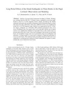
Figure 1: Observations of the pre–P signals on broadband seismometers. A) Map of the selected stations located in the 400–3000km hypocentral distance range. The red star shows the Tohoku earthquake epicenter. B) Acceleration signals aPz in the 0.002–0.03Hz frequency range, represented in a time window starting 30 minutes before the earthquake origin time and terminating at the P wave arrival at each station (1nm/s2 scale is shown to the right). Names of the station and their hypocentral distances in kilometers (following Earth surface) are shown to the left of each signal. In the time window between origin time and P wave time arrival, signals are drawn with a thick red curve. 15

INU

MDJ

Figure 2: Reconstruction of the observed elasto–gravity signals from the effects of the gravity variation and its induced acceleration. Examples at close distances (INU (GEOSCOPE) station in Japan) and at optimal distances in terms of signal observability (MDJ (IC) station in NorthEast China) are shown. The induced acceleration u¨Pz cancels the gravity variation ∆gzP at early times, and can dominate (INU) or only affect (MDJ) ∆gzP when approaching the P hypocentral time.

16

ULN 3044km

XAN 3041km

MA2 2438km

BJT 2276km

NE93 1897km

INCN 1398km

1nm/s

2

FUK 1390km

MDJ 1284km

SHR 673km

INU Tohoku observation Tohoku simulation Mw=8.5 simulation

587km

MAJO 427km

−100

0 100 200 300 Time relative to Tohoku earthquake origin time (s)

Figure 3: Agreement between observed and modeled aPz signals, and influence of the earthquake magnitude. Red (observed) and black (simulated) curves are in good agreement at all distances and azimuths from the Tohoku earthquake. The simulation for a fictitious Mw = 8.5 earthquake (dashed blue curve) shows large amplitude differences, directly illustrating the magnitude determination potential existing in these prompt elasto–gravity signals.

17

Supplementary Materials • Materials and Methods • Figs. S1 to S4 • References (32–38) • Data file S1

18

Supplementary materials for : Observations and modeling of the elasto–gravity signals preceding direct seismic waves Martin Vallée,∗ Jean Paul Ampuero, Kévin Juhel, Pascal Bernard, Jean-Paul Montagner, Matteo Barsuglia ∗

correspondence to : [email protected]

This PDF file includes: • Materials and Methods • Figs. S1 to S4 • References (32–38) Other Supplementary Materials for this manuscript include the following: Data file S1 (Trait_hplp_and_visu_SAC_for_reproduction.tar): procedure to reproduce the prompt elasto-gravity signals (shown in Figure 1), starting from the raw broadband signals. By first reading the ’README’ file of this directory, the user has : • Detailed information about the data processing strategy • A practical way to reproduce numerically the signals (starting from the raw data and metadata included in the directory), using a procedure written for the widely used SAC software. 1

Materials and Methods Modeling of the prompt elasto–gravity signals

At point r, the elastic displacement u generated by an earthquake located at rs and with normalized moment tensor Mij can be written as (e.g. 32): ui (r, t) = Mjk m(t) ∗ Gij,k (r, rs ; t)

(S1)

where Gij is the Green’s function and m is the temporal moment function of the earthquake (its integral is the earthquake seismic moment). In a realistic medium, Gij has to be calculated numerically, which is done here using AXITRA (15). This code is based on the discrete wavenumber approach (16) combined with the reflectivity technique (33), and allows to calculate the Green function in a vertically stratified medium. Earth flattening (33,34) is introduced to correct for sphericity, as some stations are several thousands of kilometers away from the earthquake. We use here the PREM model (35) in the mantle combined with a continental crustal thickness of 40 km. We use the parameters of the Global Centroid Moment Tensor (23) for the source coordinates (latitude=37.52, longitude=143.05, depth=20km), origin time (2011/03/11, 05:46:22.8) and static moment tensor Mij controlled by (strike, dip, rake) = (203◦ , 10◦ , 88◦ ). We adopt as moment function m the temporal integral of the isosceles triangular GCMT moment rate function (140 s duration). Its time integral is the GCMT seismic moment (M0 = 5.31 1022 N.m). The centroid formalism only takes into account the first order terms of the effects generated by the spatial and temporal extents of the seismic source (36). However, the source of the Tohoku earthquake is compact (250 km x 150 km , e.g. 37) and the gravity perturbations are long–period (7), hence the centroid source description is completely appropriate for most of the stations considered here. We only expect that this simplified formalism can affect the modeling accuracy at 2

the closest stations (MAJO, INU and SHR), located at distances shorter than 700 km. The latter stations are however mostly included to illustrate why their elasto-gravity signals are smaller than the ones of stations located further away (limited time window compared to earthquake duration and strong cancelling effect of the gravity perturbations by the induced accelerations), and the point-source modeling is sufficient for these purposes. At time t, the volume VsP affected by u is controlled by the travel–time of the fastest (P) elastic waves : VsP (t) = {r0 ∈ V / T P (rs , r0 ) < t},

(S2)

where V is the volume of the Earth and T P (r, r0 ) is the P–wave travel–time between r and r0 . In an homogeneous medium, VsP is an open ball, centered in rs and growing with time (Fig. S3); at t = TP , where TP = T P (rs , r0 ) is the P–wave travel–time between the source and the station located in r0 , its radius is the distance between rs and r0 . Once u is calculated using equation (S1) on a grid meshing the volume VsP (TP ), the early gravity perturbation ∆gP at times t < T P (rs , r) can be calculated with the relation (6,7): P

Z

∆g (r, t) = G VsP (t)

ρ(r0 )[u(r0 , t) − 3(er0 r .u(r0 , t))er0 r ] 0 dr |r0 − r|3

(S3)

where G is the gravitational constant, ρ is the density, and er0 r = (r0 − r)/|r0 − r|. Equation (S3) adequately takes into account the density variations in the volume due to compression and dilation, as well as the contributions of the deformation of the Earth’s surface and other material interfaces during wave propagation. Observing that ρ∆gP is instaneously non-zero everywhere in the medium (equation S3), and realizing that this term is itself a distribution of body forces generating elastic waves, there is an evolving volume VgP that is a source of elastic waves arriving in r0 before TP : ( {r0 ∈ V / T P (r0 , r0 ) < TP − t} VgP (t) = ∅ 3

if t ≥ 0 if t < 0

(S4)

In an homogeneous medium, VgP is an open ball centered in r0 , initially with radius equal to the distance between r0 and rs , and shrinking with time (Fig. S3). In any medium, there is no intersection between VgP (t) and VgP (t) for any time t (because ∀r ∈ V, (T P (r0 , r) + T P (rs , r)) ≤ TP , the only case of equality being when r is on the P ray between rs and r0 ). In VgP , the gravity perturbation is therefore the unique acting force and the associated waves arriving in r0 before TP travel in an otherwise unperturbed medium. We can then use again the Green function representation, with the gravity perturbations acting as force source terms. Taking into account the contribution of all gravity perturbations, the acceleration in r0 at t < TP is : u¨Pz (r0 , t)

d2 = 2 dt

TP

Z

Z VgP (τ )

0

ρ(r0 )∆giP (r0 , τ )Giz (r0 , r0 ; t − τ )dr0 dτ

(S5)

Considering that Giz (r0 , r0 ; t − τ ) = 0 if (t − τ ) < T P (r0 , r0 ) (before the arrival of the P waves), Equation (S5) can be written: u¨Pz (r0 , t)

d2 = 2 dt

Z 0

TP

Z VgP (t−T P (r0 ,r0 ))

ρ(r0 )∆giP (r0 , τ )Giz (r0 , r0 ; t − τ )dr0 dτ

(S6)

or in convolutive form : u¨Pz (r0 , t)

d2 = 2 dt

Z V0P (t)

ρ(r0 )∆giP (r0 , t) ∗ Giz (r0 , r0 , t)dr0

(S7)

where ( {r0 ∈ V / T P (r0 , r0 ) < t} V0P (t) = VgP (t − T P (r0 , r0 )) = ∅

if t ≤ TP if t > TP

(S8)

V0P (t) has the physical interpretation to be the location of the gravity perturbations that generate elastic waves in r0 at a given time t (< TP ). In an homogeneous medium, V0P is an open ball, centered in r0 and growing with time (Fig. S3); at t = TP , its radius is the distance between rs and r0 . In order to practically compute u¨Pz with equation (S7), ∆gP and Giz are calculated on a grid meshing V0P (TP ), using equation (S3) and again the AXITRA code, respectively.

4

Combining equations (S3) and (S7) provides access to the prompt elasto–gravity signal recorded in r0 : ∀t < TP , aPz (r0 , t) = ∆gzP (r0 , t) − u¨Pz (r0 , t)

(S9)

The theoretical cancellation between ∆gzP and u¨Pz in an homogeneous medium (see the demonstration in the last subsection of the Material and Methods) provides a way to validate the suitability of this approach in a specific case, both from the theoretical and numerical points of view. As shown in Fig. S4, this cancellation is well reproduced when deepening the source and the receiver and considering an homogeneous Earth model instead of the PREM model. This strongly supports the modeling of the elasto–gravity signals provided in this study.

Evaluation of the contribution of additional terms Other terms contributing to aPz :

In equation (S9), we neglect the additional effect on the seismometer of the gravity perturbations related to the Earth displacement uPz at the station. This additional term can be written KuPz , where the K factor represents the free–air gravity effect (2g/R, where g is gravity at the surface and R the Earth radius) minus the Bouguer anomaly (2πρG). Evaluation of these terms at the surface gives K ' 2.10−6 s−2 . When compared to u¨Pz , this term would be of comparable (or larger) amplitude only for very low frequencies, and has a quadratic decay with increasing frequencies. Practically, even at the lowest frequency considered here (0.002Hz), its relative amplitude is K/(4π 2 0.0022 ) ' 0.012. The associated perturbations are at least two orders of magnitude lower than the contributions of ∆gzP and u¨Pz considered in equation (S9).

5

Validity of the non-gravitational approximation of the wave equation

Seismological problems involving the elastic and gravitational fields can be exactly formulated by a self–gravitating set of equations where both fields are coupled (e.g. equation 4.3 in 6, coupled with the Poisson equation). This takes in particular into account that seismic waves induce gravity perturbations, which in turn modify the seismic wavefield. These effects are not considered in equations (S1) and (S5-S7), where the Green’s functions are computed with the AXITRA method in a non-gravitating medium (considering therefore the classical elasto– dynamic wave equation). However, the relative amplitude of the gravitational effects in the p wave equation at a given frequency f depends on the factor (f0 /f )2 where f0 = ρG/π (see page 142 in 6). In the crust and upper mantle, ρ = 3000 − 5000 kg/m3 , which means that even at the lowest frequencies considered here (0.002 Hz), the gravitational effects are on the order of 2%. Thus on the one hand, we can consider that inside VsP , u is accurately computed using the classical elasto–dynamic equation with a force term representing the earthquake source, which leads to equation (S1). And on the other hand, inside VgP , we can consider that u¨Pz is accurately computed using the classical elasto–dynamic equation with ρ∆gP as a body–force term (equations S5-S7). The complete resolution of the wave equations in a self-gravitating Earth, which is usually done by a normal–mode approach (e.g. 6), is therefore not required in this study. The present approach has the practical advantage to compute the prompt elasto–gravity signals without modelling the full wavefield at the station. Normal–mode summation methods would instead require a very high accuracy in order to reproduce these tiny signals without being affected by the much larger amplitude elastic waves (105 to 106 times larger, see Fig. S1)

6

¨ P in an infinite medium Full cancellation of ∆gP by u

We start from the study of Harms et al. (7), who derived the gravity perturbation ∆g induced by the seismic wavefield u generated by an earthquake source f in an infinite elastic space of density ρ0 . Ignoring self–gravitational coupling, the governing equations for that problem are: ¨ =∇·σ+f ρ0 u ∇2 ψ = −4πρ0 G ∇ · u ∆g = −∇ψ

(S10) (S11) (S12)

where σ is the stress tensor and ψ the gravitational potential. The solution features transient gravity changes before the arrival of P waves, which Harms et al. (7) coined “prompt gravity perturbations”. This prompt gravity perturbation is the restriction of the ∆g gravity perturbation to times shorter than the hypocentral P–wave arrival time at a given location, and is noted ∆gP as in the main text. Here we show that, in an infinite medium, before the arrival of “direct P waves” from the earthquake source contained in the direct wave field u, the ground acceleration ¨ P induced by ∆gP is exactly equal to ∆gP . u The momentum equation governing the gravity–induced wavefield uP , involving the stress tensor σ P , is ¨ P = ∇ · σ P + ρ0 ∆gP ρ0 u

(S13)

Because u = 0 before direct P waves arrive, we have ignored the term related to advection through the pre–existing gravity gradient ρ0 u · ∇g0 (where g0 is the initial gravity, see equation 4.3 in 6). In a self–gravitating Earth, the equations above should be solved simultaneously. p Because here we focus on frequencies significantly higher than f0 = ρ0 G/π, we can neglect the complete self–gravitational coupling and treat these equations sequentially, similarly as what has been done in the first subsection of the Material and Methods. 7

We use the conventional decomposition of the earthquake source and the direct wave field into P and S terms derived from potentials: f = ∇Φ + ∇ ∧ Ψ

(S14)

u = ∇φs + ∇ ∧ ψs

(S15)

In this formalism, P and S waves are decoupled, and a source term with a scalar potential Φ generates a pure P wave displacement with scalar potential φs . On the one hand, taking the gradient of equation (9) in Harms et al. (7), which is valid at all times, we get ∇ψ = −4πρ0 G ∇φs

(S16)

As this equation is a fortiori true before the arrival of the P waves, we have: ∆gP = 4πρ0 G ∇φs

(S17)

On the other hand, taking the gradient of equation (16) in Harms et al. (7), valid before direct P waves arrive, we get ∇ψ¨ = −4πG∇Φ

(S18)

−ρ0 ∇ψ¨ = 4πρ0 G ∇Φ ,

(S19)

Writing equation (S18) as

we recognize in the left hand side the second time derivative of the source term ρ0 ∆gP (= −ρ0 ∇ψ) that induces uP in equation (S13). Because the governing equations are linear, we infer that the wave field displacement uP induced by −ρ0 ∇ψ is related to the wave field displacement ∇φs induced by ∇Φ with ¨ P = 4πρ0 G ∇φs u

(S20)

Comparing equations (S17) and (S20), we conclude that ¨P ∆gP = u 8

(S21)

This result shows that, in an infinite medium, an accelerometer or gravimeter coupled to the elastic medium, is insensitive to the prompt gravity perturbation ∆gP because of exact ¨ P . Numerical simulations mimicking cancellation by the gravity–induced ground acceleration u the full-space configuration (Fig. S4) well reproduce this theoretical finding. However, this exact cancellation is not expected to hold in a half–space, owing to free surface effects. After the direct seismic waves reach the free surface, equation (S16) is no longer valid, but requires an additional term that involves the surface deformation (8). One particular situation is tractable and provides some insight. Before direct P waves from a buried source ¨ P is arrive at the free surface, ∆gP is the same as in an infinite space and the derivation of u still valid if in equation (S20) we replace ∇φs by the displacement field ∇φ˜s generated by ∇Φ in a half–space in the absence of ∇ ∧ Ψ. Note that ∇φ˜s is not the same as the ∇φs that may be obtained as an intermediate step in the derivation of the Green’s function for Lamb’s problem (e.g. 38), because the sources are different: ∇Φ in our problem and (∇Φ + ∇ ∧ Ψ) in Lamb’s problem. This difference is significant because P and S potentials are coupled by the free surface boundary conditions. Note also that the source ∇Φ is not localized at a point but distributed over the half space: Φ(r, t) =

Mij (t) ∂ 2 1/r 2π ∂xi ∂xj

(S22)

for a double–couple point–source (a generalization of equation 17 in Harms et al. 7). The resulting ∇φ˜s is not a pure P wave field, but includes S waves generated at the free surface. ¨ P but not to ∆gP . Clearly, in this situation, u ¨ P and ∆gP are not These S waves contribute to u equal.

9

ULN 3044km

XAN 3041km

MA2 2438km

BJT 2276km

NE93 1897km

INCN 0.1mm/s2

1398km

FUK 1390km

MDJ 1284km

1nm/s2

SHR 673km

INU 587km

MAJO

saturated

427km

−800

−600 −400 −200 0 200 Time relative to Tohoku earthquake origin time (s)

400

Figure S1: Acceleration signals in the pre– and and post–P–wave time window. Signals are filtered in the 0.002–0.03Hz frequency range, in a time window starting 800 s before the earthquake origin time and terminating 100 s after the P–wave arrival (green tick) at each station. Station names and their hypocentral distances in kilometers (following Earth surface) are shown to the left of each signal. Before the P–wave arrival, acceleration signals (aPz ) and their corresponding scales (1nm/s2 ) are shown in red (as in Figure 1). After the P–wave arrival, acceleration signals and their corresponding scales (0.1mm/s2 ) are shown in black. At this 1:100000 scale, post–P– wave signals have similar or larger amplitudes than pre–P–wave signals, meaning that the P–wave elastic signals are typically more 105 times larger than aPz . This value is even larger if comparing with later elastic arrivals (approaching 106 ), but few stations allow this comparison because of saturation of the signals. This saturation already affects the MAJO station in the 100 s time window following the P–wave arrival.

10

WEST Earth surface

EAST Tohoku earthquake

MDJ

r0

t1

Depth

div u > 0

div u < 0

t2 Figure S2: Illustration of the origins of the ∆gzP temporal variations, for stations West from the Tohoku earthquake. We here take the MDJ station (located in r0 ) as an example. The blue circles represent two isochrones of the hypocentral P–wave travel–time; the t1 isochrone illustrates early times after the earthquake origin and t2 times closer from the P–wave arrival time at MDJ. As a result of the focal mechanism of the Tohoku earthquake, the blue area is compressed by the P waves (∇·u < 0) and the green areas are dilated by the P waves (∇·u > 0). For a station located at the Earth Rsurface, there are no contributions from Earth surface effects to ∆gzP and we have ∆gzP = −G V ρ ∇ · u (err0 .ez )/r2 dr, where ez is the unit vertical vector. From the latter equation, we can figure out which parts of the volume have a dominant effect on ∆gzP at a given time t: the closest regions from the station where ∇ · u 6= 0 and err0 .ez 6= 0 are expected to be the main contributors to ∆gzP . For t = t1 and t = t2 , these regions are indicated by the red ellipses. As the sign of ∇ · u changes for these two ellipses, we expect ∆gzP to be positive at early times and to become later negative, as numerically simulated in Fig. 2.

11

A 0 < 𝑡1 < 𝑇𝑃

𝑉𝑠𝑃 𝑡1

𝑉0𝑃 𝑡1

𝑉𝑔𝑃 𝑡1

B 0 < 𝑡1 < 𝑡2 < 𝑇𝑃

𝑉𝑔𝑃 𝑡2 𝑉𝑠𝑃 𝑡2

𝑉0𝑃 𝑡2

Figure S3: Illustration of the volumes contributing to the prompt elasto–gravity signals in an homogeneous medium. The star and triangle are the earthquake and the receiver, respectively. A and B show the configuration at two increasing times before the P hypocentral arrival–time TP . VsP (shaded with red) is the volume affected by elastic displacements directly induced by the earthquake. VgP (filled with green dots) is the volume where gravitational perturbations induced by the displacements in VsP generate elastic waves arriving before TP at the receiver. V0P (t) (shaded with blue) is the volume that is at the orgin of the latter elastic waves arriving at t at the receiver. All these volumes are open balls in this homogeneous medium (where there is a full cancellation between ∆gzP and u¨Pz ). However these volumes remain defined in a realistic Earth medium (such as the PREM model used in our simulations) even if their geometries are deformed and possibly cut by the Earth surface. Even in heterogeneous media, there is no intersection between VsP and VgP . 12

Homogeneous medium

620 km

Free-air surface

600 km

A

𝑉0𝑃 𝑇𝑃 = 𝑃 𝑉𝑔 0

530 km 𝑉𝑠𝑃 𝑇𝑃

B

Figure S4: Validation of the approach in an homogeneous medium. The configuration shown in A is exactly the one of the INU station, except that (1) the earthquake and station depths have been increased by 600km and (2) the PREM model has been replaced by an homogeneous model (Vp = 6400m/s, VS = 3700m/s, ρ = 2700kg/m3 ). In this case, the 3 volumes VsP , VgP and V0P do not have any interaction with the Earth surface at any time (their maximum extensions are shown), which mimics a fully homogeneous medium. B shows that u¨Pz closely follows the evolution of ∆gzP up to the hypocentral P–wave arrival time, resulting in the expected cancellation of the elasto–gravity signal. All the signals are shown in the [0.002-0.03Hz] frequency range. 13