observations and theoretical implications of the large ... - IOPscience

A

The Astrophysical Journal, 605:78–97, 2004 April 10 # 2004. The American Astronomical Society. All rights reserved. Printed in U.S.A.

OBSERVATIONS AND THEORETICAL IMPLICATIONS OF THE LARGE-SEPARATION LENSED QUASAR SDSS J1004+4112 Masamune Oguri,1 Naohisa Inada,1 Charles R. Keeton,2 Bartosz Pindor,3 Joseph F. Hennawi,3 Michael D. Gregg,4,5 Robert H. Becker,4,5 Kuenley Chiu,6 Wei Zheng,6 Shin-Ichi Ichikawa,7 Yasushi Suto,1 Edwin L. Turner,3 James Annis,8 Neta A. Bahcall,3 Jonathan Brinkmann,9 Francisco J. Castander,10 Daniel J. Eisenstein,11 Joshua A. Frieman,2,8 Tomotsugu Goto,6,12,13 James E. Gunn,3 David E. Johnston,2 Stephen M. Kent,8 Robert C. Nichol,14 Gordon T. Richards,3 Hans-Walter Rix,15 Donald P. Schneider,16 Erin Scott Sheldon,2,17 and Alexander S. Szalay6 Received 2003 October 27; accepted 2003 December 23

ABSTRACT We study the recently discovered gravitational lens SDSS J1004+4112, the first quasar lensed by a cluster of galaxies. It consists of four images with a maximum separation of 14B62. The system was selected from the photometric data of the Sloan Digital Sky Survey (SDSS) and has been confirmed as a lensed quasar at z ¼ 1:734 on the basis of deep imaging and spectroscopic follow-up observations. We present color-magnitude relations for galaxies near the lens plus spectroscopy of three central cluster members, which unambiguously confirm that a cluster at z ¼ 0:68 is responsible for the large image separation. We find a wide range of lens models consistent with the data, and despite considerable diversity they suggest four general conclusions: (1) the brightest cluster galaxy and the center of the cluster potential well appear to be offset by several kiloparsecs; (2) the cluster mass distribution must be elongated in the north-south direction, which is consistent with the observed distribution of cluster galaxies; (3) the inference of a large tidal shear (
0.2) suggests significant substructure in the cluster; and (4) enormous uncertainty in the predicted time delays between the images means that measuring the delays would greatly improve constraints on the models. We also compute the probability of such large-separation lensing in the SDSS quasar sample on the basis of the cold dark matter model. The lack of large-separation lenses in previous surveys and the discovery of one in SDSS together imply a mass fluctuation normalization
8 ¼ 1:0þ0:4 0:2 (95% confidence) if cluster dark matter halos have an inner density profile  / r1:5 . Shallower profiles would require higher values of
8. Although the statistical conclusion might be somewhat dependent on the degree of the complexity of the lens potential, the discovery of SDSS J1004+4112 is consistent with the predictions of the abundance of cluster-scale halos in the cold dark matter scenario. Subject headings: cosmology: observations — cosmology: theory — dark matter — galaxies: clusters: general — gravitational lensing — quasars: general — quasars: individual (SDSS J100434.91+411242.8) On-line material: color figures

galaxies was originally estimated by Turner, Ostriker, & Gott (1984) to be 0.1%–1%, assuming that galaxies can be modeled as singular isothermal spheres (SIS). This prediction has been verified by several optical and radio lens surveys, such as the Hubble Space Telescope (HST ) Snapshot Survey (Bahcall et al. 1992), the Jodrell Bank / Very Large Array Astrometric Survey (JVAS; Patnaik et al. 1992), and the Cosmic Lens All Sky Survey (CLASS; Myers et al. 1995). The lensing probability is sensitive to the volume of the universe, so it can be used to place interesting constraints on the cosmological constant
 (Turner 1990; Fukugita, Futamase, & Kasai 1990;

1. INTRODUCTION Since the discovery of the first gravitationally lensed quasar, Q0957+561 (Walsh, Carswell, & Weymann 1979), about 80 strong lens systems have been found so far. All of the lensed quasars have image separations smaller than 700 , and they are lensed by massive galaxies (sometimes with small boosts from surrounding groups or clusters of galaxies). The probability that distant quasars are lensed by intervening 1 Department of Physics, University of Tokyo, Hongo 7-3-1, Bunkyo-ku, Tokyo 113-0033, Japan. 2 Astronomy and Astrophysics Department, University of Chicago, 5640 South Ellis Avenue, Chicago, IL 60637. 3 Princeton University Observatory, Peyton Hall, Princeton, NJ 08544. 4 Department of Physics, University of California at Davis, 1 Shields Avenue, Davis, CA 95616. 5 Institute of Geophysics and Planetary Physics, Lawrence Livermore National Laboratory, L-413, 7000 East Avenue, Livermore, CA 94550. 6 Department of Physics and Astronomy, Johns Hopkins University, 3701 San Martin Drive, Baltimore, MD 21218. 7 National Astronomical Observatory, 2-21-1 Osawa, Mitaka, Tokyo 181-8588, Japan. 8 Fermi National Accelerator Laboratory, P.O. Box 500, Batavia, IL 60510. 9 Apache Point Observatory, P.O. Box 59, Sunspot, NM 88349. 10 Institut d’Estudis Espacials de Catalunya/CSIC, Gran Capita 2-4, 08034 Barcelona, Spain.

11

Steward Observatory, University of Arizona, 933 North Cherry Avenue, Tucson, AZ 85721. 12 Department of Astronomy, University of Tokyo, Hongo 7-3-1, Bunkyo-ku, Tokyo 113-0033, Japan. 13 Institute for Cosmic Ray Research, University of Tokyo, 5-1-5 Kashiwa, Kashiwa City, Chiba 277-8582, Japan. 14 Department of Physics, Carnegie Mellon University, Pittsburgh, PA 15213. 15 Max-Planck Institute for Astronomy, Ko¨nigstuhl 17, D-69117 Heidelberg, Germany. 16 Department of Astronomy and Astrophysics, Pennsylvania State University, 525 Davey Laboratory, University Park, PA 16802. 17 Center for Cosmological Physics, The University of Chicago, 5640 South Ellis Avenue, Chicago, IL 60637.

78

LENSED QUASAR SDSS J1004+4112 Kochanek 1996; Chiba & Yoshii 1999; Chae et al. 2002; but see Keeton 2002). In contrast, lenses with larger image separations should probe a different deflector population: massive dark matter halos that host groups and clusters of galaxies. Such lenses therefore offer valuable and complementary information on structure formation in the universe, including tests of the cold dark matter (CDM) paradigm (Narayan & White 1988; Cen et al. 1994; Wambsganss et al. 1995; Kochanek 1995; Flores & Primack 1996; Nakamura & Suto 1997). So far the observed lack of large-separation lensed quasars has been used to infer that, unlike galaxies, cluster-scale halos cannot be modeled as singular isothermal spheres (Keeton 1998, 2001a; Porciani & Madau 2000; Kochanek & White 2001; Sarbu, Rusin, & Ma 2001; Li & Ostriker 2002, 2003; Oguri 2002; Ma 2003; Chen 2003). The difference can probably be ascribed to baryonic processes: baryonic infall and cooling have significantly modified the total mass distribution in galaxies but not in clusters (Rees & Ostriker 1977; Blumenthal et al. 1986; Kochanek & White 2001). As a result, large-separation lenses may constrain the density profiles of dark matter halos of cluster more directly than small separation lenses (Maoz et al. 1997; Keeton & Madau 2001; Wyithe, Turner, & Spergel 2001; Takahashi & Chiba 2001; Li & Ostriker 2002; Oguri et al. 2002, 2003; Huterer & Ma 2004; Kuhlen, Keeton, & Madau 2004). Alternatively, large-separation lensed quasars may be used to place limits on the abundance of massive halos if the density profiles are specified (Narayan & White 1988; Wambsganss et al. 1995; Kochanek 1995; Nakamura & Suto 1997; Mortlock & Webster 2000; Oguri 2003; Lopes & Miller 2004). Better yet, the full distribution of lens image separations may provide a systematic diagnostic of baryonic effects from small to large scales in the CDM scenario. The fact that clusters have less concentrated mass distributions than galaxies implies that large-separation lensed quasars should be less abundant than small-separation lensed quasars by 1 or 2 orders of magnitude. This explains why past surveys have failed to unambiguously identify largeseparation lensed quasars (Kochanek, Falco, & Schild 1995; Phillips, Browne, & Wilkinson 2001a; Zhdanov & Surdej 2001; Ofek et al. 2001, 2002). For instance, CLASS found 22 small-separation lenses but no large-separation lenses among
15,000 radio sources (Phillips et al. 2001b). Although several large-separation lensed quasar candidates have been found (e.g., Mortlock, Webster, & Francis 1999), they are thought to be physical (unlensed) pairs on the basis of individual observations (e.g., Green et al. 2002) or statistical arguments (Kochanek, Falco, & Mun˜oz 1999; Rusin 2002). Recently Miller et al. (2004) found six candidate lens systems with image separations  > 30 00 among
20,000 quasars in the Two-degree Field (2dF) quasar sample. Given the lack of high-resolution spectra and deep imaging for the systems, however, it seems premature to conclude that they are true lens systems. We note that because the expected number of lenses with such large image separations in the 2dF sample is much less than unity (Oguri 2003), these systems would present a severe challenge to standard models if confirmed as lenses. To find a first unambiguous large-separation lensed quasar, we started a project to search for large-separation lenses in the quasar sample of the Sloan Digital Sky Survey (SDSS; York et al. 2000). This project complements ongoing searches for small-separation lenses in SDSS (e.g., Pindor et al. 2003; Inada et al. 2003a). The SDSS has completed less than half of

79

its planned observations, but already it contains more than 30,000 quasars and is superior to previous large-separation lens surveys in several ways. The full SDSS sample will comprise
100,000 quasars, so we ultimately expect to find several large-separation lensed quasars (Keeton & Madau 2001; Takahashi & Chiba 2001; Li & Ostriker 2002; Kuhlen et al. 2004). One of the most important advantages of the SDSS in searching for large-separation lensed quasars is that imaging in five broad optical bands allows us to select lens candidates quite efficiently. Recently we reported the discovery of the large-separation lensed quasar SDSS J1004+4112 at z ¼ 1:73 (Inada et al. 2003b) in the SDSS. The quasar itself turned out to be previously identified in the ROSAT All Sky Survey (Cao, Wei, & Hu 1999) and the Two Micron All Sky Survey (Barkhouse & Hall 2001), but it was not recognized as a lensed system. Inada et al. (2003b) showed that SDSS J1004+4112 consists of four quasar images with the same redshift from the Keck spectroscopy. The colors of galaxies found by Subaru imaging follow-up observations indicated the presence of a cluster of galaxies at z ¼ 0:68. Moreover, the configuration of the four images was successfully reproduced by a simple lens model based on a singular isothermal ellipsoid mass distribution. All these results strongly implied that SDSS J1004+4112 is the first quasar lens system due to a massive cluster-scale object. In this paper we describe photometric and spectroscopic follow-up observations of SDSS J1004+4112 in detail. We discuss the spectra of lensed quasar components, including puzzling differences between emission lines seen in the different images. We analyze deep multicolor imaging data to show the existence of a lensing cluster more robustly. We also present detailed mass modeling of the lens and discuss the implications of this system for the statistics of large-separation lenses. The paper is organized as follows. Section 2 describes the method used to identify large-separation lens candidates in the SDSS data. The results of follow-up observations are summarized in x 3. In x 4 we perform mass modeling of SDSS J1004+4112, and in x 5 we consider the statistical implications of the discovery of SDSS J1004+4112. We summarize our results and conclusions in x 6. Throughout this paper, we assume the popular ‘‘concordance’’ cosmology with
M ¼ 0:27,
 ¼ 0:73, and H0 ¼ 70 km s1 Mpc1 (e.g., Spergel et al. 2003). 2. CANDIDATE SELECTION FROM THE SDSS OBJECT CATALOG The SDSS is a survey to image a quarter of the celestial sphere at high Galactic latitude and to measure spectra of galaxies and quasars found in the imaging data (Blanton et al. 2003). The dedicated 2.5 m telescope at Apache Point Observatory (APO) is equipped with a multi-CCD camera (Gunn et al. 1998) with five broad bands centered at 3561, 4676, ˚ (Fukugita et al. 1996). The imaging 6176, 7494, and 8873 A data are automatically reduced by a photometric pipeline (Lupton et al. 2001). The astrometric positions are accurate to about 0B1 for sources brighter than r ¼ 20:5 (Pier et al. 2003). The photometric errors are typically less than 0.03 mag (Hogg et al. 2001; Smith et al. 2002). The SDSS quasar selection algorithm is presented in Richards et al. (2002). The SDSS spectrographs are used to obtain spectra, covering 3800– ˚ at a resolution of 1800–2100, for the quasar candi9200 A dates. The public data releases of the SDSS are described in Stoughton et al. (2002) and Abazajian et al. (2003).

80

OGURI ET AL.

Large-separation lens candidates can be identified from the SDSS data as follows. First, we select objects that were initially identified as quasars by the spectroscopic pipeline. Specifically, among SDSS spectroscopic targets we select all objects that have spectral classification of SPEC_QSO or SPEC_ HIZ_QSO with confidence z _conf larger than 0.9 (see Stoughton et al. 2002 for details of the SDSS spectral codes). Next, we check the colors of nearby unresolved sources to see whether any of those sources could be an additional quasar image, restricting the lens search to separations  < 60 00 . We define a large-separation lens by  > 7 00 so that it exceeds the largest image separation lenses found so far: Q0957+561 with  ¼ 6B26 (Walsh et al. 1979) and RX J0921+4529 with  ¼ 6B97 (Mun˜oz et al. 2001), both of which are produced by galaxies in small clusters. We regard the stellar object as a candidate companion image if the following color conditions are satisfied: rffiffiffiffiffiffiffiffiffiffiffiffiffiffiffiffiffiffiffiffiffiffiffiffiffiffiffiffiffiffiffiffiffiffiffiffiffiffiffiffiffiffiffiffiffiffiffiffiffiffiffiffiffiffiffiffiffiffiffiffiffiffiffiffiffiffiffiffiffiffiffiffiffiffiffiffiffiffiffiffi ffi     þ
2j;err þ
2k;err ;
2j;err þ
2k;err j( j  k)j < 3
( jk ) ¼ 3 quasar

stellar

j( j  k)j < 0:1;

ð2Þ

ji j < 2:5; 









ð1Þ

ð3Þ 





18

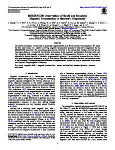
where f j; kg ¼ fu ; g g, fg ; r g, fr ; i g, and fi ; z g, and  denotes the difference between the spectroscopically identified quasar and the nearby stellar object. Note that this selection criterion is tentative; we still do not know much about large-separation lenses, so selection criteria may evolve as we learn more. Our full sample contains 44,269 quasars with the redshift distribution shown in Figure 1. For the lens search we select the subset of 29,811 quasars with 0:6 < z < 2:3, making the redshift cuts for four reasons: (1) at z < 0:6 quasars are often extended, which can complicated both lens searches and lens statistics analyses; (2) at z < 0:6 the sample is contaminated by narrow emission line galaxies; (3) at z > 2:3 we may miss a number of quasar candidates because of large color errors; and (4) lens statistics calculations for high-redshift quasars are not 18

The starred magnitudes (u g r i z ) are used to denote still-preliminary 2.5 m–based photometry (see Stoughton et al. 2002).

Fig. 1.—Redshift distribution of quasars identified by the spectroscopic pipeline in the SDSS. Dashed vertical lines show the redshift cut 0:6 < z < 2:3 used for the statistical analysis.

Vol. 605

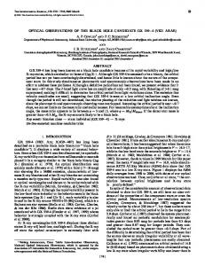
very reliable because of uncertainties in the quasar luminosity function (Wyithe & Loeb 2002a, 2002b). Lens surveys of high-redshift quasars are of course very interesting for insights into the abundance and formation of distant quasars; a search for lenses among high-redshift SDSS quasars is the subject of a separate analysis by Richards et al. (2004). SDSS J1004+4112 was first selected as a lens candidate on the basis of a pair of components, A and B (see Fig. 2), where B is the SDSS spectroscopic target. Components C and D were identified by visual inspection and found to have colors similar to those of A and B (even though they do not match the above color criteria). Table 1 summarizes the photometry for the four components, and Table 2 gives the astrometry for the four components as well as the galaxy G1 seen in Figure 2. The reason that components C and D have somewhat different colors from B is still unclear, but it must be understood in order to discuss the completeness of the lens survey. The difference might be ascribed to differential absorption or extinction by intervening material (Falco et al. 1999), or to variability in the source on timescales smaller than the time delays between the images (e.g., de Vries, Becker, & White 2003), both of which are effects that become more important as the image separation grows. 3. DATA ANALYSIS 3.1. Spectroscopic Follow-up Observations 3.1.1. Quasar Images

Since only component B has a spectrum from SDSS, we obtained spectra of the other components to investigate the lensing hypothesis. The first spectroscopic follow-up observations were done on 2003 May 2 and 5 with the Double Imaging Spectrograph of the Astrophysical Research Consortium (ARC) 3.5 m telescope at APO. All four components ˚ ) at kobs
have a prominent C iv emission line (1549.06 A ˚ , indicating that they are quasars with very similar 4230 A redshifts. Spectra with higher resolution and longer wavelength range were taken on 2003 May 30 with the LowResolution Imaging Spectrometer (LRIS; Oke et al. 1995) of the Keck I Telescope at the W. M. Keck Observatory on Mauna Kea, Hawaii. The blue grism is 400 line mm1, blazed ˚ . The red ˚ , 1.09 A ˚ pixel1, covering 3000–5000 A at 3400 A ˚ , 1.09 A ˚ pixel1, grating is 300 line mm1, blazed at 5000 A ˚ covering 5000 A to the red limit of the detector. The spectra were obtained with 900 s exposures and a 100 slit in 0B9 seeing. The data were reduced in a standard way using IRAF.19 The Keck/LRIS spectra are shown in Figure 3. All four components show emission lines of Ly, Si iv, C iv, C iii, and Mg ii. They have nearly identical redshifts of z ¼ 1:734, with velocity differences less than 50 km s1 (see Table 1). The flux ratios between the images (see Fig. 3) are almost constant over ˚ , indicating that these the wavelength range 3000–8000 A are actual lensed images. From the spectra, we conclude that the color differences found in the SDSS images are mainly caused by differences in the emission lines (discussed below) and by slightly different continuum slopes. Several absorption-line systems are seen in the spectra. Components A and D have intervening Mg ii/Fe ii absorption systems at z ¼ 0:676; this redshift is similar to that of the 19 IRAF is distributed by the National Optical Astronomy Observatories, which are operated by the Association of Universities for Research in Astronomy, Inc., under cooperative agreement with the National Science Foundation.

No. 1, 2004

LENSED QUASAR SDSS J1004+4112

81

Fig. 2.—SDSS i -band image of SDSS J1004+4112. Components A, B, C, and D are lensed images, while component G1 is the brightest galaxy in the lensing cluster.

foreground galaxies (x 3.1.2), suggesting that this absorption system is associated with the lensing galaxies. Component D has additional Mg ii absorption systems at z ¼ 0:726, 0.749, 1.083, 1.226, and 1.258. Figure 4 identifies the various Mg ii absorbers. We also note that all four components have C iv absorption lines just blueward of C iv emission lines (see Fig. 5). The velocity difference between the emission and absorption lines is
500 km s 1, so the absorption system is likely to be associated with the quasar. The fact that all four components have C iv absorption lines offers further evidence that SDSS J1004+4112 is indeed a gravitational lens.

Figure 5 shows notable differences in the C iv emission-line profiles in the different components. One possible explanation is the time delay between the lensed images; at any given observed epoch, the images represent different epochs in the source frame. However, the fact that the C iv emission lines in components A and B differ seems to rule out the time-delay explanation: the expected delay (see x 4.2.2) is shorter than the month or year timescale on which C iv emission lines typically vary (e.g., Vanden Berk et al. 2004). Other possible explanations include differences between the viewing angles probed by the images, microlensing amplification of part of the quasar

TABLE 1 Photometry of SDSS J1004+4112 Object A........................ B........................ C........................ D........................

i* 18.46 18.86 19.36 20.05

   

u*g* 0.02 0.06 0.03 0.04

0.15 0.18 0.03 0.15

   

0.05 0.08 0.05 0.09

g*r* 0.03 0.05 0.03 0.15

   

0.04 0.08 0.04 0.05

r*i* 0.24 0.23 0.38 0.46

   

0.03 0.08 0.04 0.05

i*z* 0.02 0.03 0.05 0.09

   

0.05 0.09 0.08 0.13

Redshift 1.7339 1.7335 1.7341 1.7334

   

0.0001 0.0001 0.0002 0.0003

Notes.—Magnitudes and colors for the four quasar images, taken from the SDSS photometric data. Redshifts are derived from Ly lines in the Keck LRIS spectra (see Fig. 3).

82

OGURI ET AL.

Vol. 605

TABLE 2 Astrometry of SDSS J1004+4112

Object A........................ B........................ C........................ D........................ G1......................

R.A. (J2000.0) 10 10 10 10 10

04 04 04 04 04

34.794 34.910 33.823 34.056 34.170

Decl. (J2000.0) +41 12 +41 12 +41 12 +41 12 +41 12

R.A. (arcsec)a

39.29 42.79 34.82 48.95 43.66

0.000 1.301 10.961 8.329 7.047

    

0.012 0.011 0.012 0.007 0.053

Decl. (arcsec)a 0.000 3.500 4.466 9.668 4.374

    

0.012 0.011 0.012 0.007 0.053

Notes.—Astrometry from the deep imaging data taken with Suprime-Cam (see x 3.2). The absolute coordinates are calibrated using the SDSS data. Units of right ascension are hours, minutes, and seconds, and units of declination are degrees, arcminutes, and arcseconds. a Positions relative to component A.

emission region, significant errors in the predicted time delay between A and B, or just that the quasar is extremely unusual. Understanding the puzzling line profile differences will require further observations, preferably including measurement of the time delays and spectroscopic monitoring to identify any variability in the C iv lines.

was 0B7, and the exposure time was 1740 s for both galaxies. The data were reduced in a standard way using IRAF. The spectra are shown in Figure 7. Both galaxies, denoted as G2 and G3, have z ¼ 0:675, only
700 km s 1 from the redshift of G1. 3.2. Imaging Follow-up Observations

3.1.2. Galaxies

The spectrum of the galaxy G1, the brightest object near the center of the quasar configuration (see Fig. 2), was acquired on 2003 May 30 with LRIS. The spectrum measured from a 900 s exposure is shown in Figure 6. We confirm the break ˚ . The G band also and Ca ii H and K lines at kobs
6700 A appears in the spectrum. From the Ca ii H and K and the Mg lines we derive the redshift of G1 as z ¼ 0:680. The spectra of two additional galaxies near G1 (see x 3.2) were taken on 2003 June 20 with the Faint Object Camera and Spectrograph (FOCAS; Kashikawa et al. 2002) on the Subaru 8.2 m telescope of the National Astronomical Observatory of Japan on Mauna Kea, Hawaii. We used the 300B grism together with the SY47 filter and took optical spectra covering ˚ with resolution 2.84 A ˚ pixel1. The seeing 4100–10,000 A

3.2.1. Observations

A deep r-band image of SDSS J1004+4112 was taken on 2003 May 5 with the Seaver Prototype Imaging camera of the ARC 3.5 m telescope at APO. The image shows rich structure, with many galaxies between and around the quasar components suggesting a possible galaxy cluster in the field. For a further check, we obtained deeper multicolor (griz) images on 2003 May 28 with the Subaru Prime Focus Camera (SuprimeCam; Miyazaki et al. 2002) on the Subaru 8.2 m telescope. The exposure times and limiting magnitudes of the SuprimeCam images are given in Table 3. Suprime-Cam has a pixel scale of 0B2 pixel1, and the seeing was 0B5–0B6. The frames were reduced (bias-subtracted and flat-field–corrected) in a standard way. The resulting images are shown in Figure 8. It is clear that there are many red galaxies around the four images. Moreover, we find three possible lensed arclets (distorted images of galaxies behind the cluster), which are shown in more detail in Figure 9. The fact that the arclets are relatively blue compared with the brighter galaxies in the field (see Fig. 2 in Inada et al. 2003b) suggests that the arclets may be images of distant galaxies (e.g., Colley, Tyson, & Turner 1996). Confirming that they are lensed images will require higher resolution images and measurements of the arclets’ redshifts. If the hypothesis is confirmed, the arclets will provide important additional constraints on the lens mass distribution. 3.2.2. Colors of Nearby Galaxies

Fig. 3.—Spectra (top) and flux ratios (bottom) of SDSS J1004+4112 components A, B, C, and D taken with LRIS on Keck I. In the upper panel we can confirm that all components have Ly, Si iv, C iv, C iii, and Mg ii emission lines at z ¼ 1:734. The flux ratios shown in the lower panel are almost constant for a wide range of wavelength. Several absorption lines are also seen in the spectra (see text for details). [See the electronic edition of the Journal for a color version of this figure.]

The colors of galaxies in the vicinity of SDSS J1004+4112 can help us search for the signature of a cluster. The central regions of clusters are dominated by early-type galaxies (e.g., Dressler 1980) that show tight correlations among their photometric properties (Bower, Lucey, & Ellis 1992). These correlations make it possible to search for clusters using colormagnitude and/or color-color diagrams (Dressler & Gunn 1992; Gladders & Yee 2000; Goto et al. 2002). We measure the colors of galaxies using the deep SuprimeCam griz images. Object identifications are performed using the Source Extractor algorithm (SExtractor; Bertin & Arnouts 1996); we identify objects with SExtractor parameter CLASS_STAR smaller than 0.6 in the i-band image as galaxies. Note that this star/galaxy separation criterion is successful

No. 1, 2004

LENSED QUASAR SDSS J1004+4112

83

˚ , rest-frame equivalent width Wr k 0:5 A ˚ ) of SDSS J1004+4112 Fig. 4.—Mg ii doublet absorption lines (rest-frame wavelengths of 2795.5 and 2802.7 A components A, B, C, and D at various wavelengths. The absorption lines are indicated by vertical lines. [See the electronic edition of the Journal for a color version of this figure.]

only for objects with i P 24. The magnitudes in the images are calibrated using nearby stars whose magnitudes are taken from the SDSS photometric data. Since the red galaxies in clusters are dominant in the central regions and since the center of the cluster is thought to be near G1, we divide the galaxies in the field into three categories: galaxies inside a 40 00 ; 40 00 (corresponding to 0.2 h1 Mpc ; 0:2 h1 Mpc at z ¼ 0:68) box centered on G1; galaxies

Fig. 5.—C iv lines of SDSS J1004+4112 components A, B, C, and D taken with LRIS. The associated C iv doublet absorption lines (rest-frame wave˚ , denoted by dotted lines) are seen in all four lengths 1548.2 and 1550.8 A components. [See the electronic edition of the Journal for a color version of this figure.]

inside a 100 00 ; 100 00 (0.5 h1 Mpc ; 0:5 h1 Mpc) box (except for those in the first category); and galaxies inside a 200 00 ; 200 00 (1.0 h1 Mpc ; 1:0 h1 Mpc) box (except for those ain the first two categories). Figure 10 shows colormagnitude diagrams for the three categories. It is clear that the color-magnitude relations, particularly ri and iz, show tight correlations for galaxies inside the 40 00 ; 40 00 box. Ridge lines at ri
1:1 and iz
0:5 strongly suggest a cluster of galaxies at z
0:6 (Goto et al. 2002). The result is consistent with the Keck and Subaru spectroscopic results showing that the redshifts of galaxies G1, G2, and G3 are all z
0:68.

Fig. 6.—Spectrum of the galaxy G1 taken with LRIS on Keck I. The break, Ca ii H and K absorption lines, and Mg absorption line are consistent with redshift z ¼ 0:680 (z ¼ 0:6799  0:0001 from the Ca ii H line). The G band also appears in the spectrum.

84

OGURI ET AL.

Vol. 605

Keeton (2001b). The main constraints come from the image positions. We also use the flux ratios as constraints, although we broaden the error bars to 20% to account for possible systematic effects due to source variability and time delays, micro- or millilensing, or differential extinction (See Table 4 for the full set of constraint data). In particular, the different colors of the images and the different absorption features seen in Figure 3 suggest that differential extinction may be a significant effect. In this section we do not use the position of the main galaxy as a constraint, because we want to understand what constraints can be placed on the center of the lens potential from the lens data alone. We first consider the simplest possible models for a fourimage lens: an isothermal lens galaxy with a quadrapole produced either by ellipticity in the galaxy or by an external shear. A spherical isothermal lens galaxy has surface mass density (r) ¼

Fig. 7.—Spectra of galaxies G2 and G3 taken with FOCAS on the Subaru 8.2 m telescope. From the absorption lines Ca ii H and K, H , and G band, we find that the redshifts of both galaxies are z ¼ 0:675 (z ¼ 0:6751  0:0001 from the H lines).

We identify cluster members by their location in color-color space (Dressler & Gunn 1992; Goto et al. 2002). We show gri and riz color-color diagrams in Figures 11 and 12, respectively. We restrict the plots to galaxies brighter than i ¼ 24 because of the limitation of the star/galaxy separation. We make color-color cuts on the basis of the colors expected of elliptical galaxies (Fukugita, Shimasaku, & Ichikawa 1995): gr > 1:5, ri > 0:7, and iz > 0:2 for elliptical galaxies at z k 0:5. The galaxy distributions with and without the color cuts are shown in Figure 13. The galaxies that survive the color cuts are concentrated around G1, so we conclude that they are candidate members of a cluster of galaxies at z ¼ 0:68 whose center is near G1. We note that the distribution of candidate cluster members is not spherical and appears to be elongated north-south. 4. MASS MODELING 4.1. One-Component Models To search for mass models that can explain the image configuration of SDSS J1004+4112, we use standard lens modeling techniques as implemented in the software of TABLE 3 Subaru Observations Band

Exposure Time

mlima

g.................................. r .................................. i .................................. z ..................................

810 1210 1340 180

27.0 26.9 26.2 24.0

Notes.—Total exposure time in seconds and limiting magnitude (mlim) for the Subaru deep imaging observations. a Defined by S=N > 5 for point sources.

(r) rEin ; ¼ crit 2r

ð4Þ

where rEin is the Einstein radius of the lens and crit ¼ (c2 =4G ) (Dos =Dol Dls ) is the critical surface mass density for lensing, with Dol, Dol, and Dls being angular diameter distances from the observer to the lens, from the observer to the source, and from the lens to the source, respectively. The Einstein radius is related to the velocity dispersion
of the galaxy by 
2 D ls : ð5Þ rEin ¼ 4 c Doc  For an elliptical model we replace r with r 1 þ ½ (1  q2 )=(1 þ q2 ) cos 2(  e )g1=2 in the surface density, where q and e are the axis ratio and position angle of the ellipse. Simple models using either pure ellipticity or pure shear fail miserably, yielding 2 values no better than 2 ; 104 for Ndof ¼ 4 degrees of freedom. This failure is not surprising: most four-image lenses require both ellipticity and external shear (e.g., Keeton, Kochanek, & Seljak 1997), and such a situation is likely in SDSS J1004+4112 since the main galaxy is observed to be elongated and the surrounding cluster surely contributes a shear. We therefore try models consisting of a singular isothermal ellipsoid (SIE) plus an external shear . Even though such models are still comparatively simple, they can fit the data very well with a best-fit value of 2 ¼ 0:33 for Ndof ¼ 2. The best-fit model has an Einstein radius rEin ¼ 6B9 ¼ 35 h1 kpc corresponding to a velocity dispersion of 700 km s1, an ellipticity e ¼ 0:50 at position angle e ¼ 21:4, and an external shear  ¼ 0:25 at position angle  ¼ 60:9. Among other known lenses, such a large shear is found only in lenses lying in cluster environments (Burud et al. 1998; Barkana et al. 1999). Figure 14 shows the critical curves and caustics for the bestfit model. The inferred source position lies very close to the caustic and fairly near a cusp, implying that the total magnification is
57. Figure 15 shows the allowed ranges for the position of the deflector and the ellipticity and external shear in the model. The models indicate a small but significant offset of 1B6 ¼ 7:9 h1 kpc between the center of the lens potential and the main galaxy, although it remains to be seen whether that offset is real or an artifact of these still simple lens models. 4.2. Two-Component Models Even though the simple SIE+shear model provides a good fit to the data, we believe that it is not physically plausible

No. 1, 2004

LENSED QUASAR SDSS J1004+4112

85

Fig. 8.—Deep griz images taken with Suprime-Cam on the Subaru 8.2 m telescope. The exposure details are summarized in Table 3.

because the system clearly has multiple mass components and it seems unlikely that all of the mass is associated with a single
700 km s1 isothermal component. The next level of complication is to add a mass component representing the cluster halo. We still model the galaxy G1 explicitly, treating it as an isothermal ellipsoid constrained by its observed position. At this point we do not further complicate the model by attempting to treat the other galaxies within the lens explicitly.

where the lensing strength is specified by the parameter

4.2.1. Methods

We model the cluster component with an NFW profile that has been predicted in cosmological N-body simulations (Navarro, Frenk, & White 1996, 1997): (r) ¼

crit (z) c (z) ðr=rs Þð1 þ r=rs Þ2

1997, 2001, 2003; Power et al. 2003; Fukushige, Kawai, & Makino 2004; Hayashi et al. 2004), we adopt this form for simplicity. The lensing properties of a spherical NFW halo are described by the lens potential (Bartelmann 1996; Golse & Kneib 2002; Meneghetti, Bartelmann, & Moscardini 2003a)  qffiffiffiffiffiffiffiffiffiffiffiffiffiffiffiffiffiffiffiffiffi  2 r 2 2  arctan h 1  (r=rs )2 ; ð7Þ

(r) ¼ 2s rs ln 2rs

;

ð6Þ

where rs is a scale radius, c is a characteristic overdensity (which depends on redshift), and crit (z) is the critical density of the universe. Although the NFW density profile appears to deviate from the results of more recent N-body simulations in the innermost region (Moore et al. 1999; Ghigna et al. 2000; Jing & Suto 2000; Klypin et al. 2001; Fukushige & Makino

s ¼

rs c (z)crit (z) : crit

ð8Þ

Since asphericity in the cluster potential is important in modeling this system, we generalize the spherical model by adopting elliptical symmetry in the potential. Making the potential (rather than the density) elliptical makes it possible to compute the lensing properties of an NFW halo analytically (Golse & Kneib 2002; Meneghetti et al. 2003a). We may still be oversimplifying the mass model, because the cluster profile may have been modified from the NFW form by baryonic processes such as gas cooling (Rees & Ostriker 1977; Blumenthal et al. 1986), and the cluster may have a complex

86

OGURI ET AL.

Vol. 605

Fig. 9.—Central region of the Suprime-Cam i-band image. The galaxies with measured redshifts (G1 from LRIS and G2 and G3 from FOCAS) as well as the four lensed images are labeled. The possible lensed arclets are marked with rectangles.

angular structure if it is not relaxed (e.g., Meneghetti et al. 2003a). To allow for the latter possibility, we still include a tidal shear in the lens model that can approximate the effects of complex structure in the outer parts of the cluster. Overall, our goal is not to model all of the complexities of the lens potential but to make the minimal realistic model and see what we can learn. Even with our simplifying assumptions, we still have a complex parameter space with 11 parameters defining the lens potential: the mass, ellipticity, and position angle for the galaxy G1; the position, mass, scale radius, ellipticity, and position angle for the cluster; and the amplitude and position angle of the shear. There are also three parameters for the source (position and flux). With just 12 constraints (position and flux for each of four images), the models are underconstrained. We therefore expect that there may be a range of lens models that can fit the data. To search the parameter space and identify the range of models, we follow the technique introduced by Keeton & Winn (2003) for many-parameter lens modeling. Specifically, we pick random starting points in the parameter space and then run an optimization routine to find a (local) minimum in the 2 surface. Repeating that process numerous times should reveal different minima and thereby

sample the full range of models. Many of the recovered models actually lie in local minima that do not represent good fits to the data, so we keep only recovered models with 2 < 11:8 (which represents the 3
limit relative to a perfect fit when examining two-dimensional slices of the allowed parameter range; see Press et al. 1992). We make one further cut on the models. From the previous section, we know that an SIE+shear lens model can give a good fit to the data. Thus, there are acceptable two-component models where most or all of the mass is in the galaxy component and the cluster contribution is negligible. To exclude such models as physically implausible, we impose an upper limit on the velocity dispersion of the model galaxy. Specifically, we only keep models with
gal < 400 km s1, because there are essentially no galaxies in the observed universe with larger velocity dispersions, even in rich clusters (e.g., Kelson et al. 2002; Bernardi et al. 2003; Sheth et al. 2003). Formally, we impose this cut as an upper limit rEin < 2B25 on the Einstein radius of the galaxy G1. 4.2.2. Results

We first consider models where the scale radius of the cluster is fixed as rs ¼ 40 00 (we shall justify this choice

No. 1, 2004

LENSED QUASAR SDSS J1004+4112

87

Fig. 12.—Similar to Fig. 11, but for riz. [See the electronic edition of the Journal for a color version of this figure.]

Fig. 10.—Color-magnitude diagrams for the SDSS J1004+4112 field taken with Suprime-Cam. We divide the galaxies into three categories according to their positions: filled circles denote galaxies inside a 40 00 ; 40 00 box centered on G1, open triangles denote galaxies inside a 100 00 ; 100 00 box, and crosses denote galaxies inside a 200 00 ; 200 00 box. These box sizes correspond to 0.2 h1 Mpc ; 0:2 h1 Mpc, 0.5 h1 Mpc ; 0:5 h1 Mpc, and 1.0 h1 Mpc ; 1:0 h1 Mpc at z ¼ 0:68, respectively. Three spectroscopically confirmed member galaxies are marked with open circles. The corresponding r-band absolute magnitudes at z ¼ 0:68 (without K-correction) are given at the top of the frame. [See the electronic edition of the Journal for a color version of this figure.]

Fig. 11.—The gri color-color diagram of galaxies brighter than i ¼ 24. Symbols are the same as in Fig. 10. Dotted lines indicate color cuts to find cluster members. [See the electronic edition of the Journal for a color version of this figure.]

below). Figure 16 shows the allowed parameter ranges for acceptable models. First, Figure 16a shows that the cluster component is restricted to a fairly small (but not excessively narrow) range of positions near the center of the image configuration. This is mainly a result of our upper limit on the mass of the galaxy component; there is a certain enclosed mass implied by the image separation, and if the galaxy cannot contain all of that mass, then the cluster component must lie within the image configuration to make up the difference. It is interesting to note that even in these more complicated models there still seems to be a small offset between the center of the cluster component and the brightest cluster galaxy G1, although the lower limit implied by our models is just 0B71 ¼ 3:6 h1 kpc. Figure 16b shows that the allowed values for the ellipticity and position angle of the galaxy G1 basically fill the parameter space, so these parameters are not constrained by the lens data. We might want to impose an external constraint, however. Analyses of other lens systems show that the lensing mass is typically aligned with the projected light distribution (Keeton, Kochanek, & Falco 1998; Kochanek 2002). We may therefore prefer lens models where the model galaxy is at least roughly

Fig. 13.—Distributions of galaxies brighter than i ¼ 24 with (right) and without (left) the color cut. The origin (0; 0) is set to the position of the central galaxy G1. Filled squares denote the four lensed images.

88

OGURI ET AL.

Vol. 605

TABLE 4 Constraints on Mass Models

Object A......................... B......................... C......................... D......................... G1.......................

xa (arcsec) 0.000 1.301 10.961 8.329 7.047

    

0.012 0.011 0.012 0.007 0.053

ya (arcsec) 0.000 3.500 4.466 9.668 4.374

    

0.012 0.011 0.012 0.007 0.053

Fluxb (arbitrary) 1.0 0.682 0.416 0.195

 0.2  0.136  0.083  0.039 ...

P.A.c (deg) ... ... ... ... 19.9

Notes.—Summary of positions, flux ratios, and position angles (P.A.) of SDSS J1004+4112 used in the mass modeling. a The positive directions of x and y are defined by west and north, respectively. b Errors are broadened to 20% to account for possible systematic effects. c Degrees measured east of north.

aligned with the observed galaxy, which has a position angle of 19:9. To illustrate this possible selection, we show all models but highlight those where the position angle of the model galaxy is in the range e ¼ 19:9  20:0. The broad 20 uncertainties prevent this constraint from being too strong. Figure 16c shows that there are some acceptable models where the cluster potential is round, but most models have some ellipticity that is aligned roughly north-south. This is in good agreement with the distribution of member galaxies, which is also aligned roughly north-south (see Fig. 13). The ellipticity e
0:2–0.4 is actually quite large, considering that this parameter describes the ellipticity of the potential, not that of the density. Figure 16d shows that all of the acceptable models require a fairly large tidal shear  k 0:10, and models where the galaxy is aligned with the observed galaxy have a strong shear  k 0:23. The shear tends to be aligned east-west. The fact that the models want both a large cluster ellipticity and a large tidal shear strongly suggest that there is complex structure in the cluster potential outside of the image configuration. It would be interesting to see whether there is any evidence for such structure in, for example, X-rays from the cluster. Figure 17 shows critical curves and caustics for sample lens models. The critical curves are not well determined. The outer, tangential critical curve can point either northeast (e) or northwest (d), or it can have a complex shape (a). Sometimes there is just one inner, radial critical curve (e), but often there are two (c). The distance of the source from the caustic (and of the images from the critical curve) varies from model to model, so the total magnification can range from
50 to

Fig. 14.—Critical curve (left) and caustic (right) for the best-fit SIE+shear lens model of SDSS J1004+4112. In the left panel the filled circles mark the image positions, the open circle indicates the observed position of the brightest cluster galaxy G1, and the cross marks the best-fit deflector position. In the right panel the filled circle marks the inferred source position.

several hundred, or even more. Finally, perhaps the most interesting qualitative result is that even the image parities are not uniquely determined. In most models (e.g., a–f ) images A and D lie inside the critical curve and have negative parity while B and C lie outside the critical curve and have positive parity. However, in some models (e.g., g–h) the situation is reversed. Having ambiguous image parities is very rare in lens modeling. So far we have only discussed models where the cluster has a scale radius rs ¼ 40 00 . We have also computed models with rs ¼ 1000 , 2000 , 3000 , 5000 , and 6000 , and we find that all of the results are quite similar. To understand what value of the scale radius is reasonable, we must consider which (if any) of the models have physically plausible cluster parameters. Even though NFW models are formally specified by two parameters, rs and s, N-body simulations reveal that the two parameters are actually correlated. NFW models therefore appear to form a one-parameter family of models, although with some scatter that reflects the scatter of the concentration parameter cvir ¼ rvir =rs (rvir is a virial radius of the cluster). Figure 18 shows the predicted relation between rs and s, including the scatter. For comparison, it also shows the fitted values of s in lens models with different scale radii. Models with rs ¼ 10 00 or 2000 require values of s much larger than expected, corresponding to a halo that is too concentrated. Models with rs  30 00 , by contrast, overlap with the predictions and thus are physically plausible. We can therefore conclude very roughly that the cluster component must have rs k 30 00 and a total virial mass M k1014 h1 M. Finally, we can use the models to predict the time delays between the images. The models always predict that the time

Fig. 15.—Likelihood contours drawn at 1, 2, and 3
for various parameter combinations in SIE+shear lens models. The left panel shows constraints on the position of the deflector; the circle marks the observed position of the main galaxy. The right panel shows contours in the ellipticity-external shear plane.

No. 1, 2004

LENSED QUASAR SDSS J1004+4112

89

Fig. 16.—Allowed parameter ranges for galaxy+cluster lens models with a cluster scale radius rs ¼ 40 00 . (a) The position of the cluster component. The filled circles mark the image positions, and the open circle marks the observed brightest cluster galaxy G1. (b) The ellipticity and position angle of the galaxy component. (c) The ellipticity and position angle of the cluster component. (d) The amplitude and position angle of the external shear. Small points show all models, while boxes mark models where the model galaxy is roughly aligned with the observed galaxy (e ¼ 19:9  20:0).

delay between images C and D is the longest and the delay between A and B is the shortest. However, there is no robust prediction of the temporal ordering: most models predict that the sequence should be C-B-A-D, but a few models predict the reverse ordering D-A-B-C. This is a direct result of the ambiguity in the image parities, because the leading image is always a positive-parity image (e.g., Schneider, Ehlers, & Falco 1992). We note, however, that all of the models where the model galaxy is roughly aligned with the observed galaxy have the C-B-A-D ordering. Figure 19 shows the predictions for the long and short time delays. The long delay between C and D can be anything up to
3000 h 1 days, while the short delay between A and B can be up to
37 h1 days. For the models where the galaxy is roughly aligned with the observed galaxy, the two delays are approximately proportional to each other, with tCD =tBA ¼ 143  16. These results have several important implications. First, the A-B time delay should be on the order of weeks or months, so it should be very feasible to measure it, provided that the source has detectable variations. Measuring the A-B delay would be very useful because it would determine the temporal ordering and thereby robustly determine the image parities. In addition, it would allow a good estimate of the long C-D delay

and indicate whether attempting to measure that delay would be worthwhile. Second, the enormous range of predicted time delays means that constraining the Hubble constant with this system (Refsdal 1964) will be difficult because of large systematic uncertainties in the lens models. Although Koopmans et al. (2003) recently showed that it is possible to obtain useful constraints on the Hubble constant even in a complex system with two mass components, the analysis is very complex and requires extensive data including not just the image positions and all of the time delays, but also an Einstein ring image and the velocity dispersion of one of the mass components. Even if we obtain such data for SDSS J1004+4112 in the near future, it seems likely that it will be difficult to obtain reliable constraints on the Hubble constant given the complexity of the lens potential in SDSS J1004+4112. The time delays, however, would still be extremely useful, because they would determine the temporal ordering and hence the image parities, and they would provide constraints that can rule out many of the models that are currently acceptable. 5. LENS STATISTICS In this section we calculate the expected rate of largeseparation lensing in the SDSS quasar sample. The discovery of

90

OGURI ET AL.

Vol. 605

Fig. 17.—Critical curves and caustics for sample galaxy+cluster lens models with a cluster scale radius rs ¼ 40 00 . In each panel the left-hand side shows the critical curves in the image plane and the right-hand side shows the caustics in the source plane on the same scale. The points in the image plane show the observed image positions, and the point in the source plane shows the inferred source position. The value of gives the total magnification in each model.

SDSS J1004+4112 allows us to move past the upper limits obtained from previous large-separation lens searches, although at present the main thing we can do is test whether the detection of one large-separation lens in the current sample is consistent with standard theoretical models in the CDM scenario. 5.1. Modeling Lens Probabilities We calculate lensing probabilities using spherical models for simplicity. Although halos in CDM simulations are in fact triaxial (e.g., Jing & Suto 2002), the spherical assumption is often adopted in lens statistics calculations because deviations from spherical symmetry mainly affect image multiplicities, not image separations or the total optical depth for lensing (e.g., Kochanek 1996; Keeton et al. 1997; Chae 2003). While this result has been obtained for isothermal lens potentials, checking it for more general halos is beyond the scope of this paper and is the subject of a follow-up analysis (M. Oguri et al. 2004, in preparation). 5.1.1. Lens Probabilities

Let the physical image position in the lens plane and physical source position in the source plane as  and ,

respectively. Consider the probability that a quasar at zS with luminosity L is strongly lensed. The probability of lensing with image separation larger than  is given by Z Z zs c dt 1 dn
lens B(zs ; L) dzl (1 þ zl )3 dM PB (> ; zs ; L) ¼ dzl Mmin dM 0 ð9Þ where
lens ¼  r2 D2ol =D2os is the cross section for lensing, with r being the physical radius of the radial caustic in the source plane. The lower limit of the mass integral is the mass Mmin that corresponds to the image separation ; this can be computed once the density profile of the lens object is specified. The magnification bias B(zS ; L) is (Turner 1980; Turner et al. 1984) Z r 2 1 ; ð10Þ B(zs ; L) ¼ 2 d ½ zs ; L= ( ) r (zs ; L) 0

( ) where (zs ; L) is the luminosity function of source quasars. Note that the magnification factor ( ) may be interpreted as the total magnification or the magnification of the brighter or

No. 1, 2004

LENSED QUASAR SDSS J1004+4112

91

5.1.2. Generalized NFW Profile

The lensing probability distribution at large separation reflects the properties of dark halos rather than galaxies (Keeton & Madau 2001; Takahashi & Chiba 2001; Li & Ostriker 2002; Oguri 2002). For the statistics calculation, the debate over the inner slope of the density profile seen in N-body simulations leads us to consider the generalized version (Zhao 1996; Jing & Suto 2000) of the NFW density profile (eq. [6]): (r) ¼

Fig. 18.—Relation between the cluster scale radius rs and lensing strength s. The solid line shows the predicted relation for clusters with the canonical median concentration, and the dotted lines show the 1
range due to the scatter in concentration (see x 5.1.2). The labeled points show the value of log (M ) (in units of h1 M) at various points along the curve. The points show fitted values of s for lens models with rs ¼ 1000 , 2000 , 3000 , 4000 , 5000 , and 6000 . As in Fig. 16, small points show all models, while boxes mark models where the model galaxy is roughly aligned with the observed galaxy.

crit (z) c (z) ðr=rs Þ ð1 þ r=rs Þ3

:

ð11Þ

While the correct value of  is still unclear, the existence of cusps with 1 P  P 1:5 has been established in recent N-body simulations (Navarro et al. 1996, 1997; Moore et al. 1999; Ghigna et al. 2000; Jing & Suto 2000; Klypin et al. 2001; Fukushige & Makino 1997, 2001, 2003; Power et al. 2003; Fukushige et al. 2004; Hayashi et al. 2004). The case  ¼ 1 corresponds to the original NFW profile, while the case  ¼ 1:5 resembles the profile proposed by Moore et al. (1999). The scale radius rs is related to the concentration parameter as cvir ¼ rvir =rs . Then the characteristic density c (z) is given in terms of the concentration parameter: c (z) ¼

vir (z)
(z) c3vir ; 3 m(cvir )

ð12Þ

where m(cvir ) is fainter image, depending on the observational selection criteria (Sasaki & Takahara 1993; Cen et al. 1994). In this paper we adopt the magnification of the fainter image, because we concentrate on the large-separation lenses for which the images are completely deblended.

m(cvir ) ¼

c3 vir 3

2

F1 ð 3   ; 3   ; 4  ; cvir Þ;

ð13Þ

with 2 F1 ð a; b; c; xÞ being the hypergeometric function (e.g., Keeton & Madau 2001). The mean overdensity vir (z) can be computed using the nonlinear spherical collapse model (e.g., Nakamura & Suto 1997). We define ˜ =rs and ˜ Dol =rs Dos . Then the lensing ˜ is related to the dark halo profile as deflection angle () follows: ˜ ¼ 4s () ˜

Z

Z

1

˜

dz 0

0

x dx pffiffiffiffiffiffiffiffiffiffiffiffiffiffi  pffiffiffiffiffiffiffiffiffiffiffiffiffiffi3 : 2 2 x þz 1 þ x2 þ z 2 ð14Þ

The lensing strength parameter s was defined in equation (8). For sources inside the caustic ( < r ), the lens equation has three solutions ˜1 > ˜2 > ˜3 , where image 1 is on the same side of the lens as the source and images 2 and 3 are on the opposite side.20 The lens image separation is then ¼

rs (˜1 þ ˜2 ) 2rs ˜t ’ ; Dol Dol

ð15Þ

where ˜t is a radius of the tangential critical curve (Hinshaw & Krauss 1987; Oguri et al. 2002). The magnification of the fainter image may be approximated by (Oguri et al. 2002) Fig. 19.—Predictions for the longest (tCD ) and shortest (tBA ) time delays, where tij > 0 means image i leads image j and vice versa. Results are shown for models where the cluster has scale length rs ¼ 30 00 , 4000 , 5000 , and 6000 . As in Fig. 16, small points show all models, while boxes mark models where the model galaxy is roughly aligned with the observed galaxy. [See the electronic edition of the Journal for a color version of this figure.]

˜t

:

faint ( ) ’ ˜ 1   0 (˜t ) 20

ð16Þ

The third image is usually predicted to be very faint, so in practice just two images are actually observed.

92

OGURI ET AL.

These approximations are sufficiently accurate over the range of interest here (see Oguri et al. 2002). Although we adopt a selection criterion that the flux ratios should be smaller than 10 : 1, this condition does not affect our theoretical predictions because the flux ratios of strong lensing by NFW halos are typically much smaller than 10 : 1 (Oguri et al. 2002; Rusin 2002). The concentration parameter cvir depends on a halo’s mass and redshift. Moreover, even halos with the same mass and redshift show significant scatter in the concentration, which reflects the difference in formation epoch (Wechsler et al. 2002) and is well described by a lognormal distribution. For the median of this distribution, we adopt the mass and redshift dependence reported by Bullock et al. (2001) as a canonical model:   10 M 0:13 ; ð17Þ cBullock (M ; z) ¼ 1 þ z M (0) where M (z) is the mass collapsing at redshift z [defined by
M (z) ¼ c 1:68]. To study uncertainties related to the concentration distribution, we also consider other mass and redshift dependences, e.g., cCHM (M ; z) ¼ 10:3(1 þ z)0:3



M M (z)

Vol. 605

by equation (20) with A ¼ 0:22, B ¼ 0:73, and  ¼ 3:86 in terms of the mean overdensity  c ¼ 200=
(z) (Evrard et al. 2002); and the mass function given by Sheth & Tormen (1999),   2 p  dnSTW
M crit (0)
(z) 1þ M 2 ¼A M a c dM rffiffiffiffiffiffi   2a c d ln
1 a 2 M exp  2 c ; ; ð21Þ 
M (z) dM 2
M (z) with A ¼ 0:29, a ¼ 0:66, and p ¼ 0:33 in terms of the mean overdensity c ¼ 180 (White 2002). 5.2. Number of Lensed Quasars in the SDSS Because the lensing probability depends on the source redshift and luminosity, we compute the predicted number of lenses in redshift and luminosity bins and then sum the bins. Specifically, let N (zj ; ik ) be the number of quasars in a redshift range zj  z=2 < z < zj þ z=2 that have a magnitude in the range ik  i =2 < i < ik þ i =2. Then the predicted total number of lensed quasars is XX

N (zj ; ik )P > ; zj ; L(ik ) : ð22Þ Nlens (> ) ¼ zj

0:24(1þz)0:3 ;

from Cooray, Hu, & Miralda-Escude´ (2000), and sffiffiffiffiffiffiffiffiffiffiffiffiffiffiffiffi vir (zc ) 1 þ zc 3=2 ; cJS (M; z) ¼ 2:44 vir (z) 1 þ z

ð18Þ

ð19Þ

from Jing & Suto (2002), with zc being the collapse redshift of the halo of mass Mvir . Note that these relations were derived under the assumption of  ¼ 1. We can extend them to  6¼ 1 by multiplying the concentration by a factor 2   (Keeton & Madau 2001; Jing & Suto 2002). The statistics of large-separation lenses are highly sensitive to the degree of scatter in the concentration (Keeton & Madau 2001; Wyithe et al. 2001; Kuhlen et al. 2004). Bullock et al. (2001; see also Wechsler et al. 2002) found
c
0:32 in their simulations. Jing (2000) found a smaller scatter
c
0:18 among well-relaxed halos, but Jing & Suto (2002) found
c
0.3 if all halos are considered. Therefore we use
c ¼ 0:3 throughout the paper.

ik

We adopt bins of width z ¼ 0:1 and i ¼ 0:2. The quasar sample we used comprises 29,811 quasars with mean redshift hzi ¼ 1:45 (see Fig. 1) and roughly corresponds to a sample with magnitude limit i ¼ 19:1 (Richards et al. 2002). To calculate the B-band absolute luminosity L(i ) corresponding to observed magnitude i , we must estimate the cross-filter K-correction KBi (z). The K-correction calculated from the composite quasar spectrum created from the SDSS sample by Vanden Berk et al. (2001) is shown in Figure 20. As a simplification, one might use the following approximation:  7500  0:12; KBi (z) ¼ 2:5(1   s ) log (1 þ z)  2:5 s log 4400 ð23Þ where the offset 0.12 mainly arises from the difference between AB(4400) and B magnitudes (calculated assuming

5.1.3. Mass Function

For the comoving mass function of dark matter halos, unless otherwise specified we adopt equation (B3) of Jenkins et al. (2001): dnJenkins
M crit (0) d ln
1 

M ¼A exp jln
1 M (z) þ Bj ; M dM dM ð20Þ where A ¼ 0:301, B ¼ 0:64, and  ¼ 3:82. We use the approximation of
M given by Kitayama & Suto (1996) and the shape parameter presented by Sugiyama (1995). Note that this mass function is given in terms of the mean overdensity c ¼ 180 instead of vir (z). Therefore, the mass function should be converted correctly (e.g., Komatsu & Seljak 2002). To study uncertainties related to the mass function we also consider two other possibilities: the mass function derived in the Hubble volume simulations, dnEvrard =dM , which is given

Fig. 20.—Cross-filter K-correction, computed from the SDSS composite quasar spectrum created by Vanden Berk et al. (2001). Dotted line indicate the approximation (eq. [23]) with  s ¼ 0:5.

No. 1, 2004

LENSED QUASAR SDSS J1004+4112

93

 s ¼ 0:5; Schmidt et al. 1995). Throughout the paper, however, we use the K-correction directly calculated from composite quasar spectrum. The luminosity function of quasars is needed to compute magnification bias. We adopt the standard double power-law B-band luminosity function (Boyle, Shanks, & Peterson 1988) (zs ; L)dL ¼

 l

h

½L=L (zs ) þ ½L=L (zs )

dL : L (zs )

ð24Þ

As a fiducial model of the evolution of the break luminosity, we assume the form proposed by Madau, Haardt, & Rees (1999), L (zs ) ¼ L (0)(1 þ zs ) S 1

ezs (1 þ ez ) ; ezs þ ez

ð25Þ

where a power-law spectral distribution for quasar spectrum has been assumed, f /   s . Wyithe & Loeb (2002b) determined the parameters so as to reproduce the low-redshift luminosity function as well as the space density of high-redshift quasars for a model with h ¼ 3:43 below zs ¼ 3, h ¼ 2:58 above zs ¼ 3, and l ¼ 1:64. The resulting parameters are  ¼ 624 Gpc3 , L (0) ¼ 1:50 ; 1011 L , z ¼ 1:60,  ¼ 2:65, and  ¼ 3:30. We call this model LF1. To estimate the systematic effect, we also use another quasar luminosity function (LF2) derived by Boyle et al. (2000) (h ¼ 3:41, l ¼ 1:58) and2 an evolution of the break luminosity L (zs ) ¼ L (0)10k1 zS þk2 zS with k1 ¼ 1:36, k2 ¼ 0:27, and M ¼ 21:15 þ 5 log h. 5.3. Results First we show the conditional probability distributions

2

d P=dzl d dP

; ð26Þ (zl j; zs ; L)

dzl dP=d

2

d P=d ln Md dP

; (M j; zs ; L) ð27Þ

d ln M dP=d in order to identify the statistically reasonable ranges of redshift and mass for the lensing cluster. Figure 21 shows the conditional probability distribution of the lens redshift, and Figure 22 shows the conditional probability distribution of the lens mass, given that the gravitational lens system SDSS J1004+4112 has image separation
1400 , source redshift zs ¼ 1:734, and apparent magnitude i ¼ 18:86. We find the most probable lens redshift to be zl
0:5, but the distribution is broad and the measured redshift zl ¼ 0:68 is fully consistent with the distribution. We also find a cluster mass M
2– 3 ; 1014 h1 M to be most probable for this system. This result is in good agreement with the mass estimated from the lens models (see Fig. 18). Note that we do not include information on the measured redshift zl ¼ 0:68 in Figure 22, which might cause a slight underestimate of the lens mass. Next we consider the statistical implications of SDSS J1004+4112. Although our large-separation lens search is still preliminary and we have several other candidates from the current SDSS sample that still need follow-up observations, we can say that the current sample contains at least one largeseparation lens system. This is enough for useful constraints because of the complementary constraints available from the lack of large-separation lenses in previous lens surveys. Among the previous large-separation lens surveys, we adopt the CLASS 6 00 <  < 15 00 survey comprising a statistically

Fig. 21.—Conditional probability distributions for the lens redshift in SDSS J1004+4112, given the image separation
1400 , source redshift zs ¼ 1:739, and apparent magnitude i ¼ 18:86. Solid and dashed lines show the probability distributions with  ¼ 1:5 and 1.0, respectively. The arrow shows the measured redshift of the lensing cluster. We assume
8 ¼ 1:0.

complete sample of 9284 flat-spectrum radio sources (Phillips et al. 2001b). For the CLASS sample, we use a source redshift zs ¼ 1:3 (Marlow et al. 2000) and a flux distribution N (S)dS / S 2:1 dS (Phillips et al. 2001b) to compute the expected number of large-separation lenses. Figure 23 shows contours of the predicted number of largeseparation lenses with  > 7 00 in the SDSS quasar sample. Since the number of lenses is very sensitive to both the inner slope of the density profile  and the mass fluctuation normalization
8 (e.g., Oguri 2002), we draw contours in the ( ;
8 ) plane. Constraints from the existence of SDSS J1004+4112 together with the lack of large-separation lenses in the CLASS sample are shown in Figure 24. To explain both observations, we need a relatively large  or
8, such as
8 ¼ 1:0þ0:4 0:2 (95% confidence) for  ¼ 1:5. This value is consistent with other observations, such as cosmic microwave background anisotropies (Spergel et al. 2003). By contrast, if we adopt  ¼ 1, then the required value of
8 is quite large,
8 k 1:1. Thus, our result might be interpreted as implying

Fig. 22.—Same as Fig. 21, but the conditional probability distribution of the mass of the lens is plotted.

94

OGURI ET AL.

Fig. 23.—Contours of the predicted number of large-separation ( > 7 00 ) lenses in the current SDSS sample in the (;
8 ) plane.

that dark matter halos have cusps steeper than  ¼ 1. Alternatives to collisionless CDM, such as self-interacting dark matter (Spergel & Steinhardt 2000) or warm dark matter (Bode, Ostriker, & Turok 2001), tend to produce less concentrated mass distributions that are effectively expressed by low ; such models would fail to explain the discovery of SDSS J1004+4112 unless
8 is unexpectedly large. This result is consistent with results from strong lensing of galaxies by clusters (i.e., giant arcs), which also favors the collisionless CDM model (Smith et al. 2001; Meneghetti et al. 2001; Miralda-Escude´ 2002; Gavazzi et al. 2003; Oguri, Lee, & Suto 2003; Wambsganss et al. 2004; Dalal, Holder, & Hennawi 2004; but see Sand et al. 2004 for different conclusion). We note that the abundance of large-separation lenses produces a degeneracy between  and
8 seen in Figure 24, but additional statistics such as the distribution of time delays can break the degeneracy (Oguri et al. 2002).

Fig. 24.—Constraints from both SDSS and CLASS in the ( ;
8 ) plane. The discovery of one large-separation ( > 7 00 ) lens in SDSS provides lower limits on  and
8, while the lack of large-separation lenses (6 00 <  < 15 00 ) in CLASS yields the upper limit. The regions in which both SDSS and CLASS limits are satisfied are shown by the shadings. The confidence levels are 68.3%, 95.5%, and 99.7% in the dark, medium, and light shaded regions, respectively. [See the electronic edition of the Journal for a color version of this figure.]

Vol. 605

Table 5 summarizes the sensitivity of our predictions to various model parameters. The uncertainties in our predictions are no more than a factor of 2–3, dominated by uncertainties in the concentration parameter and the matter density
M . This error roughly corresponds to 
8
0:1 and so does not significantly change our main results. There may be larger systematic errors associated with effects we have not considered in this paper. For example, triaxiality in cluster halos is very important in arc statistics because it can dramatically increase the length of the tangential caustic that gives rise to giant arcs (Oguri et al. 2003; Meneghetti et al. 2003a; Dalal et al. 2004). The effect would seem to be less important in the statistics of lensed quasars, which depend mainly on the area enclosed by the radial caustic, but it still needs to be examined quantitatively. The presence of a central galaxy is thought to have a small impact on arc statistics (Meneghetti et al. 2003b), but the complexity of the lens potentials we found in our mass modeling suggests that the effect of the galaxy on the statistics of lensed quasars also needs to be considered. 6. SUMMARY AND CONCLUSION We have presented the candidate selection and follow-up observations of the first cluster-scale lensed quasar, SDSS J1004+4112. The system consists of four components with image separation 
14 00 and was selected from the largeseparation lens search in the SDSS. The spectroscopic and photometric follow-up observations confirm SDSS J1004+ 4112 to be a lens system; spectroscopic observations of four components showed that they have nearly identical spectra with z ¼ 1:734. Deep images and spectroscopy of nearby galaxies indicate that there is a cluster of galaxies with z ¼ 0:68, whose center is likely to be among the four components. We conclude that the cluster is responsible for this largeseparation lens. Differences between the C iv emission-line profiles in the four images remain puzzling, and it will be interesting to reobserve the profiles at several epochs to search for variability that might explain the differences. We have shown that reasonable mass models can successfully reproduce the observed properties of the lens. When we consider models that include both the cluster potential and the brightest cluster galaxy, we find a broad range of acceptable models. Despite the diversity in the models, we find several general and interesting conclusions. First, there appears to be a small (k4 h1 kpc) offset between the brightest cluster galaxy and the center of the cluster potential. Such an offset is fairly common in clusters (e.g., Postman & Lauer 1995). Second, the cluster potential is inferred to be elongated roughly north-south, which is consistent with the observed distribution of apparent member galaxies. Third, we found that a significant external shear 
0:2 is needed to fit the data, even when we allow the cluster potential to be elliptical. This may imply that the structure of the cluster potential outside of the images is more complicated than simple elliptical symmetry. Fourth, given the broad range of acceptable models, we cannot determine even the parities and temporal ordering of the images, much less the amplitudes of the time delays between the images. Measurements of any of the time delays would therefore provide powerful new constraints on the models. We note that the complexity of the lens potential means that the time delays will be more useful for constraining the mass model than for trying to measure the Hubble constant. Our modeling results suggest that further progress will require new data (rather than refinements of current data). The

No. 1, 2004

LENSED QUASAR SDSS J1004+4112

95

TABLE 5 Systematic Effects Nlens(>700 ) for (,
8) Models

(1.0, 0.7)

(1.5, 0.7)

(1.0, 1.1)

(1.5, 1.1)

Fiducial model ................................ cBullock ! cCHM ............................... cBullock ! cJS ................................... dnJenkins =dM ! dnSTW =dM ............ dnJenkins =dM ! dnEvrard =dM .......... LF1 ! LF2 .....................................
M ¼ 0:27 ! 0:22 .........................
M ¼ 0:27 ! 0:32 .........................

0.0027 0.00002 0.00049 0.0044 0.00075 0.0024 0.00066 0.0083

0.071 0.0097 0.065 0.11 0.026 0.066 0.027 0.15

0.47 0.16 0.17 0.53 0.22 0.42 0.24 0.81

3.0 1.8 2.4 3.2 1.7 2.8 1.8 4.6

Notes.—Sensitivity of the predicted number of large-separation lensed quasars in the SDSS quasar sample to various changes in the statistics calculations.

interesting possibilities include catalogs of confirmed cluster members, X-ray observations, and weak-lensing maps, not to mention measurement of time delays and confirmation of lensed arcs (either the possible arclets we have identified or others). For instance, with an estimated cluster mass of M
3 ; 1014 h1 M, the estimated X-ray bolometric flux is SX
1013 ergs s1 cm2, which means that the cluster should be accessible with the Chandra and XMM-Newton X-ray observatories; the excellent spatial of Chandra may be particularly useful for separating the diffuse cluster component from the bright quasar images (which have a total X-ray flux SX
2 ; 1012 ergs s1 cm 2 in the ROSAT All Sky Survey). The confirmation of lensed arclets would be very valuable, as they would provide many more pixels’ worth of constraints on the complicated lens potential. In principle, mapping radio jets in the quasar images could unambiguously reveal the image parities (e.g., Gorenstein et al. 1988; Garrett et al. 1994), but unfortunately the quasar appears to be radio-quiet since it is not detected in radio sky surveys such as the FIRST survey (Becker, White, & Helfand 1995). Although the large-separation lens search in the SDSS is still underway, we can already constrain model parameters from the discovery of SDSS J1004+4112. The existence of at least one large-separation lens in SDSS places a lower limit on the lensing probability that complements the upper limits from previous surveys. Both results can be explained if clusters have the density profiles predicted in the collisionless CDM scenario and moderate values of the mass fluctuation parameter
8. In particular we find
8 ¼ 1:0þ0:4 0:2 (95% confidence), assuming that the inner density profile of dark matter halos has the form  / r with  ¼ 1:5. The value of
8 is, however, degenerate with  such that smaller values of  require larger values of
8. Various systematic errors are estimated to be 
8
0:1, dominated by uncertainties in the distribution of the concentration parameter cvir and in the matter density parameter
M. Other systematic effects, such as triaxiality in the cluster potential and the presence of a central galaxy, remain to be considered. Still, our overall conclusion is that the discovery of SDSS J1004+4112 is fully consistent with the standard model of structure formation (i.e., CDM with
8
1). In summary, SDSS J1004+4112 is a fascinating new lens system that illustrates how large-separation lenses can be used to probe the properties of clusters and test models of structure formation. The full SDSS sample is expected to contain several more large-separation lenses. The complete sample of lenses, and the distribution of their image separations, will be

extremely useful for understanding the assembly of structures from galaxies to clusters. More immediately, the discovery of a quasar lensed by a cluster of galaxies fulfills longestablished theoretical predictions and resolves uncertainties left by previously unsuccessful searches. We thank Don York for valuable comments on the manuscript and an anonymous referee for many useful suggestions. Part of the work reported here was done at the Institute of Geophysics and Planetary Physics, under the auspices of the US Department of Energy by Lawrence Livermore National Laboratory under contract W-7405-Eng-48. Funding for the creation and distribution of the SDSS archive has been provided by the Alfred P. Sloan Foundation, the Participating Institutions, the National Aeronautics and Space Administration, the National Science Foundation, the US Department of Energy, the Japanese Monbukagakusho, and the Max Planck Society. The SDSS Web site is http://www.sdss.org. The SDSS is managed by the Astrophysical Research Consortium (ARC) for the Participating Institutions. The Participating Institutions are the University of Chicago, Fermilab, the Institute for Advanced Study, the Japan Participation Group, the Johns Hopkins University, Los Alamos National Laboratory, the Max Planck Institute for Astronomy (MPIA), the Max Planck Institute for Astrophysics (MPA), New Mexico State University, the University of Pittsburgh, Princeton University, the United States Naval Observatory, and the University of Washington. This work is based in part on data collected at Subaru Telescope, which is operated by the National Astronomical Observatory of Japan. Some of the Data presented herein were obtained at the W. M. Keck Observatory, which is operated as a scientific partnership between the California Institute of Technology, the University of California, and the National Aeronautics and Space Administration. The Observatory was made possible by the generous financial support of the W. M. Keck Foundation. This work is also based in part on observations obtained with the Apache Point Observatory 3.5 m telescope, which is owned and operated by the Astrophysical Research Consortium. We thank the staffs of Subaru, Keck, and APO 3.5 m telescopes for their excellent assistance. The authors wish to recognize and acknowledge the very significant cultural role and reverence that the summit of Mauna Kea has always had within the indigenous Hawaiian community. We are most fortunate to have the opportunity to conduct observations from this mountain.

96

OGURI ET AL.

Vol. 605

REFERENCES Abazajian, K., et al. 2003, AJ, 126, 2081 Keeton, C. R. 2002, ApJ, 575, L1 Bahcall, J. N., Maoz, D., Doxsey, R., Schneider, D. P., Bahcall, N. A., Keeton, C. R., Kochanek, C. S., & Falco, E. E. 1998, ApJ, 509, 561 Lahav, O., & Yanny, B. 1992, ApJ, 387, 56 Keeton, C. R., Kochanek, C. S., & Seljak, U. 1997, ApJ, 482, 604 Barkana, R., Leha´r, J., Falco, E. E., Grogin, N. A., Keeton, C. R., & Shapiro, I. I. Keeton, C. R., & Madau, P. 2001, ApJ, 549, L25 1999, ApJ, 520, 479 Keeton, C. R., & Winn, J. N. 2003, ApJ, 590, 39 Barkhouse, W. A., & Hall, P. B. 2001, AJ, 121, 2843 Kelson, D. D., Zabludoff, A. I., Williams, K. A., Trager, S. C., Mulchaey, J. S., Bartelmann, M. 1996, A&A, 313, 697 & Bolte, M. 2002, ApJ, 576, 720 Becker, R. H., White, R. L., & Helfand, D. J. 1995, ApJ, 450, 559 Kitayama, T., & Suto. Y. 1996, ApJ, 469, 480 Bernardi, M., et al. 2003, AJ, 125, 1817 Klypin, A., Kravtsov, A. V., Bullock, J. S., & Primack, J. R. 2001, ApJ, Bertin, E., & Arnouts, S. 1996, A&AS, 117, 393 554, 903 Blanton, M. R., Lin, H., Lupton, R. H., Maley, F. M., Young, N., Zehavi, I., & Kochanek, C. S. 1995, ApJ, 453, 545 Loveday, J. 2003, AJ, 125, 2276 ———. 1996, ApJ, 466, 638 Blumenthal, G. R., Faber, S. M., Flores, R., & Primack, J. R. 1986, ApJ, ———. 2002, in Proc. Workshop, The Shapes of Galaxies and their Halos, ed. 301, 27 P. Natarjan (Singapore: World Scientific), 62 Bode, P., Ostriker, J. P., & Turok, N. 2001, ApJ, 556, 93 Kochanek, C. S., Falco, E. E., & Mun˜oz, J. A. 1999, ApJ, 510, 590 Bower, R. G., Lucey, J. R., & Ellis, R. S. 1992, MNRAS, 254, 601 Kochanek, C. S., Falco, E. E., & Schild, R. 1995, ApJ, 452, 109 Boyle, B. J., Shanks, T., Croom, S. M., Smith, R. J., Miller, L., Loaring, N., & Kochanek, C. S., & White, M. 2001, ApJ, 559, 531 Heymans, C. 2000, MNRAS, 317, 1014 Komatsu, E., & Seljak, U. 2002, MNRAS, 336, 1256 Boyle, B. J., Shanks, T., & Peterson, B. A. 1988, MNRAS, 235, 935 Koopmans, L. V. E., Treu, T., Fassnacht, C. D., Blandford, R. D., & Surpi, G. Bullock, J. S., Kolatt, T. S., Sigad, Y., Somerville, R. S., Kravtsov, A. V., 2003, ApJ, 599, 70 Klypin, A. A., Primack, J. R., & Dekel, A. 2001, MNRAS, 321, 559 Kuhlen, M., Keeton, C. R., & Madau, P. 2004, ApJ, 601, 104 Burud, I., et al. 1998, ApJ, 501, L5 Li, L. X., & Ostriker, J. P. 2002, ApJ, 566, 652 Cao, L., Wei, J.-Y., & Hu, J.-Y. 1999, A&AS, 135, 243 ———. 2003, ApJ, 595, 603 Cen, R., Gott, J. R., Ostriker, J. P., & Turner, E. L. 1994, ApJ, 423, 1 Lopes, A. M., & Miller, L. 2004, MNRAS, submitted (astro-ph/0306174) Chae, K.-H. 2003, MNRAS, 346, 746 Lupton, R., Gunn, J. E., Ivezic´, Z., Knapp, G. R., Kent, S., & Yasuda, N. Chae, K.-H., et al. 2002, Phys. Rev. Lett., 89, 151301 2001, in ASP Conf. Ser. 238, Astronomical Data Analysis Software and Chen, D. 2003, ApJ, 587, L55 Systems X, ed. F. R. Harnden, Jr., F. A. Primini, & H. E. Payne (San Francisco: Chiba, M., & Yoshii, Y. 1999, ApJ, 510, 42 ASP), 269 Colley, W. N., Tyson, J. A., & Turner, E. L. 1996, ApJ, 461, L83 Ma, C.-P. 2003, ApJ, 584, L1 Cooray, A., Hu, W., & Miralda-Escude´, J. 2000, ApJ, 535, L9 Madau, P., Haardt, F., & Rees, M. J. 1999, ApJ, 514, 648 Dalal, N., Holder, G., & Hennawi, J. F. 2004, ApJ, submitted (astro-ph/ Maoz, D., Rix, H.-W., Gal-Yam, A., & Gould, A. 1997, ApJ, 486, 75 0310306) Marlow, D. R., Rusin, D., Jackson, N., Wilkinson, P. N., & Browne, I. W. A. de Vries, W. H., Becker, R. H., & White, R. L. 2003, AJ, 126, 1217 2000, AJ, 119, 2629 Dressler, A. 1980, ApJ, 236, 351 Meneghetti, M., Bartelmann, M., & Moscardini, L. 2003a, MNRAS, 340, 105 Dressler, A., & Gunn, J. E. 1992, ApJS, 78, 1 ———. 2003b, MNRAS, 346, 67 Evrard, A. E., et al. 2002, ApJ, 573, 7 Meneghetti, M., Yoshida, N., Bartelmann, M., Moscardini, L., Springel, V., Falco, E. E., et al. 1999, ApJ, 523, 617 Tormen, G., & White S. D. M. 2001, MNRAS, 325, 435 Flores, R. A., & Primack, J. R. 1996, ApJ, 457, L5 Miller, L., Lopes, A. M., Smith, R. J., Croom, S. M., Boyle, B. J., Shanks, T., & Fukugita, M., Futamase, T., & Kasai, M. 1990, MNRAS, 246, 24P Outram, P. 2004, MNRAS, in press (astro-ph/0210644) Fukugita, M., Ichikawa, T., Gunn, J. E., Doi, M., Shimasaku, K., & Schneider, Miralda-Escude´, J. 2002, ApJ, 564, 60 D. P. 1996, AJ, 111, 1748 Miyazaki, S., et al. 2002, PASJ, 54, 833 Fukugita, M., Shimasaku, K., & Ichikawa, T. 1995, PASP, 107, 945 Moore, B., Quinn, T., Governato, F., Stadel, J., & Lake, G. 1999, MNRAS, Fukushige, T., Kawai, A., & Makino, J. 2004, ApJ, submitted (astro-ph/ 310, 1147 0306203) Mortlock, D. J., & Webster, R. L. 2000, MNRAS, 319, 872 Fukushige, T., & Makino, J. 1997, ApJ, 477, L9 Mortlock, D. J., Webster, R. L., & Francis, P. J. 1999, MNRAS, 309, 836 ———. 2001, ApJ, 557, 533 Mun˜oz, J. A., et al. 2001, ApJ, 546, 769 ———. 2003, ApJ, 588, 674 Myers, S. T., et al. 1995, ApJ, 447, L5 Garrett, M. A., Calder, R. J., Porcas, R. W., King, L. J., Walsh, D., & Nakamura, T. T., & Suto, Y. 1997, Prog. Theor. Phys., 97, 49 Wilkinson, P. N. 1994, MNRAS, 270, 457 Narayan, R., & White, S. D. M. 1988, MNRAS, 231, 97P Gavazzi, R., Fort, B., Mellier, Y., Pello, R., & Dantel-Fort, M. 2003, A&A, Navarro, J. F., Frenk, C. S., & White, S. D. M. 1996, ApJ, 462, 563 403, 11 ———. 1997, ApJ, 490, 493 Ghigna, S., Moore, B., Governato, F., Lake, G., Quinn, T., & Stadel, J. 2000, Ofek, E. O., Maoz, D., Prada, F., Kolatt, T., & Rix, H.-W. 2001, MNRAS, ApJ, 544, 616 324, 463 Gladders, M. D., & Yee, H. K. C. 2000, AJ, 120, 2148 Ofek, E. O., Rix, H.-W., Maoz, D., & Prada, F. 2002, MNRAS, 337, 1163 Golse, G. & Kneib, J.-P. 2002, A&A, 390, 821 Oguri, M. 2002, ApJ, 580, 2 Gorenstein, M. V., Cohen, N. L., Shapiro, I. I., Rogers, A. E. E., Bonometti, ———. 2003, MNRAS, 339, L23 R. J., Falco, E. E., Bartel, N., & Marcaide, J. 1988, ApJ, 334, 42 Oguri, M., Lee, J., & Suto, Y. 2003, ApJ, 599, 7 Goto, T., et al. 2002, AJ, 123, 1807 Oguri, M., Taruya, A., Suto, Y., & Turner, E. L. 2002, ApJ, 568, 488 Green, P. J., et al. 2002, ApJ, 571, 721 Oke, J. B., et al. 1995, PASP, 107, 375 Gunn, J. E., et al. 1998, AJ, 116, 3040 Patnaik, A. R., Browne, I. W. A., Wilkinson, P. N., & Wrobel, J. M. 1992, Hayashi, E., et al. 2004, MNRAS, submitted (astro-ph/0310576) MNRAS, 254, 655 Hinshaw, G., & Krauss, L. M. 1987, ApJ, 320, 468 Phillips, P. M., Browne, I. W. A., & Wilkinson, P. N. 2001a, MNRAS, 321, 187 Hogg, D. W., Finkbeiner, D. P., Schlegel, D. J., & Gunn, J. E. 2001, AJ, Phillips, P. M., et al. 2001b, MNRAS, 328, 1001 122, 2129 Pier, J. R., Munn, J. A., Hindsley, R. B., Hennessy, G. S., Kent, S. M., Huterer, D., & Ma, C.-P. 2004, ApJ, 600, L7 Lupton, R. H., & Ivezic´, Zˇ. 2003, AJ, 125, 1559 Inada, N., et al. 2003a, AJ, 126, 666 Pindor, B., Turner, E. L., Lupton, R. H., & Brinkmann, J. 2003, AJ, 125, 2325 ———. 2003b, Nature, 426, 810 Porciani, C., & Madau, P. 2000, ApJ, 532, 679 Jenkins, A., Frenk, C. S., White, S. D. M., Colberg, J. M., Cole, S., Evrard, Postman, M., & Lauer, T. R. 1995, ApJ, 440, 28 A. E., Couchman, H. M. P., & Yoshida, N. 2001, MNRAS, 321, 372 Power, C., Navarro, J. F., Jenkins, A., Frenk, C. S., White, S. D. M., Jing, Y. P. 2000, ApJ, 535, 30 Springel, V., Stadel, J., & Quinn, T. 2003, MNRAS, 338, 14 Jing, Y. P., & Suto, Y. 2000, ApJ, 529, L69 Press, W. H., Teukolsky, S. A., Vetterling, W. T., & Flannery, B. P. 1992, ———. 2002, ApJ, 574, 538 Numerical Recipes in Fortran (Cambridge: Cambridge Univ. Press) Kashikawa, N., et al. 2002, PASJ, 54, 819 Rees, M. J., & Ostriker, J. P. 1977, MNRAS, 179, 541 Keeton, C. R. 1998, Ph. D. thesis, Harvard Univ. Refsdal, S. 1964, MNRAS, 128, 307 ———. 2001a, ApJ, 561, 46 Richards, G. T., et al. 2002, AJ, 123, 2945 ———. 2001b, preprint (astro-ph/0102340) ———. 2004, AJ, submitted (astro-ph/0309274)

No. 1, 2004

LENSED QUASAR SDSS J1004+4112

Rusin, D. 2002, ApJ, 572, 705 Sand, D. J., Treu, T., Simth, G. P., & Ellis, R. S. 2004, ApJ, in press (astro-ph/ 0309465) Sarbu, N., Rusin, D., & Ma, C.-P. 2001, ApJ, 561, L147 Sasaki, S., & Takahara, F. 1993, MNRAS, 262, 681 Schmidt, M., Schneider, D. P., & Gunn, J. E. 1995, AJ, 110, 68 Schneider, P., Ehlers, J., & Falco, E. E. 1992, Gravitational Lenses (New York: Springer) Sheth, R. K., & Tormen, G. 1999, MNRAS, 308, 119 Sheth, R. K., et al. 2003, ApJ, 594, 225 Smith, G. P., Kneib, J., Ebeling, H., Czoske, O., & Smail, I. 2001, ApJ, 552, 493 Smith, J. A., et al. 2002, AJ, 123, 2121 Spergel, D. N., & Steinhardt P. J. 2000, Phys. Rev. Lett., 84, 3760 Spergel, D. N., et al. 2003, ApJS, 148, 175 Stoughton, C., et al. 2002, AJ, 123, 485 Sugiyama, N. 1995, ApJS, 100, 281 Takahashi, R., & Chiba, T. 2001, ApJ, 563, 489 Turner, E. L. 1980, ApJ, 242, L135

97

Turner, E. L., 1990, ApJ, 365, L43 Turner, E. L., Ostriker, J. P., & Gott, J. R. 1984, ApJ, 284, 1 Vanden Berk, D. E., et al. 2001, AJ, 122, 549 ———. 2004, ApJ, 601, 692 Walsh, D., Carswell, R. F., & Weymann, R. J. 1979, Nature, 279, 381 Wambsganss, J., Bode, P., & Ostriker, J. P. 2004, ApJ, submitted (astro-ph/ 0306088) Wambsganss, J., Cen, R., Ostriker, J. P., & Turner, E. L. 1995, Science, 268, 274 Wechsler, R. H., Bullock, J. S., Primack, J. R., Kravtsov, A. V., & Dekel, A. 2002, ApJ, 568, 52 White, M. 2002, ApJS, 143, 241 Wyithe, J. S. B., & Loeb, A. 2002, Nature, 417, 923 ———. 2002, ApJ, 577, 57 Wyithe, J. S. B., Turner, E. L., & Spergel, D. N. 2001, ApJ, 555, 504 York, D. G., et al. 2000, AJ, 120, 1579 Zhao, H. S. 1996, MNRAS, 278, 488 Zhdanov, V. I., & Surdej, J. 2001, A&A, 372, 1