observations of snow particle size distribution with 2-d video

P2.5

OBSERVATIONS OF SNOW PARTICLE SIZE DISTRIBUTION WITH 2-D VIDEO DISDROMETER AND POLARIMETRIC RADAR Sean Luchs

*1,2

1,2

3

2

2

, Guifu Zhang , Alexander Ryzhkov ,Ming Xue , Lily Ryzhkova , Qing Cao 1 Atmospheric Radar Research Center, Norman, Oklahoma 2 School of Meteorology, University of Oklahoma, Norman, Oklahoma 3 National Severe Storms Laboratory, Norman, Oklahoma

1. INTRODUCTION Across much of the United States, and in many parts of the world, winter precipitation can come in many forms. It can range from all-liquid rain, to partially frozen particles, and completely frozen particles such as ice pellets or snow. The results of winter precipitation, then, are highly dependent on what type of precipitation falls. If rain falls into subfreezing environments, can down power lines and destroy trees, potentially paralyzing day-to-day life. Snow can block roadways and high accumulations can put large amounts of pressure on man-made structures (Stewart 1992). Winter storms are responsible for billions of dollars of damage, and can cause significant injury and death (Cortinas et al 2004, Cortinas 2000). Conceptually, rain and snow are relatively predictable compared to other forms of winter precipitation. A common situation occurs following the passage of a surface cold front (or ahead of a warm front), where a shallow layer of cold air at the surface sits below a melting layer. Freezing rain falls when particles that become liquid in the melting layer do not refreeze in the cold layer but do freeze upon reaching the surface. If the particles do refreeze before hitting the ground, ice pellets fall at the surface. This process can be very complex, and see varying degrees of melting (Zerr 1997). An event can have freezing rain or ice pellets exclusively, periods of each, and the two may even coexist (Stewart 1992). Winter precipitation can be observed using in situ measurements, such as rain and snow gauges, as well as disdrometers. They can also be observed with remote sensing instruments, such as satellites and radars (both airborne and ground-based). In general, rain events are studied more commonly than winter events (Henson 2007). While studies of frozen and liquid hydrometeors using polarimetric radar or ____________________ Corresponding author address: Sean Luchs, School of Meteorology, University of Oklahoma, 120 David L. Boren Blvd., Suite 5900 Norman, OK 73072. E-mail: [email protected]

1,2

disdrometers are often focused on rain and hail in summer thunderstorms, polarimetric radar data can be used to analyze winter events. Trapp et al (2001) is one such study, using polarimetric radar to observe a winter storm event with snow and mixed-phase precipitation in Oklahoma. Brandes et al (2007) studies the microphysics of snow in Colorado using a 2D video disdrometer. Studies using both polarimetric radar and disdrometer data follow a similar pattern. Investigations for rain events are more numerous (for example, Goddard et al 1982, Schuur et al 2001, Bringi et al 2003, Bringi et al 2006, Thurai et al 2007, Cao et al, 2008). Snow, on the other hand, has been studied considerably less (Ibrahaim et al 1998, though Löffler-Mang and Blahak 2001 and Tokay et al 2007 compare disdrometer data with radar using solely horizontal polarization). These studies, however, focus on events or portions of events where dry snow is the predominant hydrometeor. Thurai et al (2007), which concentrated on a cold rain event, did briefly describe a later period of mixed phase precipitation the following day. In contrast, data collected by the polarimetric radar KOUN and the University of Oklahoma 2D video disdrometer (OU 2DVD) during the winter of 20062007 contained contributions from all-liquid, allfrozen, and mixed phase precipitation. Measurements from the disdrometer are used to determine the precipitation microphysics, including drop size distributions (DSDs) and particle size distributions (PSDs) for liquid precipiation and precipitation containing frozen particles, respectively. A model is used to “melt” data from periods of frozen precipitation in order to compare distributions, water contents, and precipitation rates with periods of rain from the same event. This comparison can help support work in improving species transition in modeling. The disdrometer data can is also used to model the reflectivity factor (Z) and differential reflectivity factor (ZDR) in order to be compared with KOUN data above the location of the disdrometer. This work will help understand connections between radar and ground measurements, and be used to support work in improving rainfall estimates by polarimetric radar.

This paper begins with a basic description of the instrumentation used in the observation of winter precipitation in Central Oklahoma, as well as the events during the winter of 2006-2007 which make up the dataset. Afterwards, the methods used to calculate the polarimetric variables from the disdrometer data are discussed. Following that is an introduction to the two melting models used to investigate a snow-rain transition. The polarimetric variables calculated from the disdrometer data are then compared to radar measurements. Finally, the melting models are applied to snow particle size distributions and compared to disdrometer measurements of rain portion of the events. 2. INSTRUMENTATION AND DATASET 2.1 KOUN Polarimetric Radar The National Severe Storms Laboratory operates a research WSR-88D radar, KOUN, in Norman, Oklahoma. KOUN was outfitted with dual-polarization capabilities in 2002 in advance of the upcoming conversion of the NEXRAD network to dual-polarization. The radar is linearly polarized, and simultaneously transmits and receivers horizontally-polarized and verticallypolarized waves (Ryzhkov et al 2005). The polarimetric variables available from KOUN are the standard WSR-88D products (radar reflectivity factor, Z; Doppler velocity, V; spectral width, σv), and additional polarimetric variables differential reflectivity (ZDR), differential phase (ΦDP), and cross-correlation coefficient (ρhv). These polarimetric variables and their observation have been discussed extensively, including Doviak and Zrnić (1993), Herzegh and Jameson (1992), Zrnić and Ryzhkov (1999), and Straka et al (2000). The two measurements used in this study are reflectivity factor, Z (or Zhh), and differential reflectivity, ZDR. 2.2 2D Video Disdrometer The OU 2DVD was deployed on land operated by the University of Oklahoma, the Kessler Farm Field Laboratory (KFFL). KFFL is approximately 30 km from KOUN. At this distance, the disdrometer lies beyond the region of ground clutter, but is still close enough to the radar to ensure good resolution. In addition, the Washington site of the Oklahoma Mesonet is also located at KFFL, allowing for collection of surface observations nearby (Chilson et al 2007). The disdrometer is manufactured by Joanneum Research at the Austrian Institute for Applied Systems Technology. The instrument is

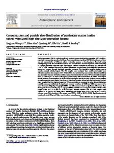
Fig. 1. Representative particles as measured by the OU 2DVD on November 30, 2006. The top panel shows a rain drop, the middle shows an ice pellet, and the bottom panel shows a snowflake.

thoroughly described by Kruger and Kajewski (2002), and again following the design of a lowprofile version by Schönhuber et al (2008) – thus, only the most significant details will be presented here. The operation of the 2DVD is based on two orthogonal sheets of light projected onto line-scan cameras. These two sheets are spaced 6.2 mm apart. The cameras measure particles as they fall through the sheets of light, and measure both the size of the particles, as well as the time it takes or a particle to fall through the sheet in order to calculate its fall velocity. From this data, the disdrometer can also calculate the equivolume sphere diameter, rain rate, and drop size distribution over one minute intervals. At the time of publication by Schönhuber (2008), the OU 2DVD was one of 22 such disdrometers in use. The OU 2DVD is an example of the low-profile version of this disdrometer. Figure 1 shows different types of precipitation from November 30, 2006 as measured by the disdrometer. 2.3 Dataset Data from KOUN were collected during several precipitation events during the 2006-2007 winter. These events had rain, snow, or mixed phase precipitation, and several had periods of multiple types. Radar data for the location of the

disdrometer is an average of a 3x3 box of resolution volumes from the 0.5 degree elevation scan centered on the volume located above the location of the disdrometer. Radar data was available for all periods of precipitation during these events, with the exception of a period of rain on January 27, 2007. During these same events, there is data from the OU2DVD that was also collected. During the events for which KOUN data was collected, there were 7752 one minute particle size distributions measured by the disdrometer. For a more stable distribution, particularly during periods of snow, these were condensed into five minute distributions. There were four events for which radar and disdrometer data were collected: November 30, 2006; January 12-14, 2007; January 27, 2007; and February 15, 2007. The first three events contained transitions from liquid precipitation to frozen precipitation, while only snow fell during the February 15 event. The precipitation associated with the November 30 event began with convection along a cold front, and continued with stratiform precipitation. The early precipitation was primarily rain, which eventually transitioned into mixed phase precipitation. This gave way to ice pellets, and ended with a period of snow (Scharfenberg et al 2007). Many schools and businesses closed as a result of this storm, including the University of Oklahoma campus. The January 12-14 event was similar in character – however, after a short, initial period of rain, there was mixed phase precipitation through the remainder of the event, with no snow. This storm also had serious consequences, not only in Oklahoma, but throughout much of the United States and parts of Canada. Like the previous two events, the precipitation on January 27 was again in the wake of the passage of a cold front. The initial precipitation following the cold front fell as rain. After this rain fell, there was a brief break in precipitation, and then a second swath of snow fell. The February 15 event was different from the others in that there was only snowfall associated with this system, which fell well in advance of the passage of a low pressure system. 3. Methodology & Physical Models

Z h ,v =

4λ4

π 4 Kw

∫

2

f h ,v ( D) N ( D)dD , (1)

where λ is the radar wavelength, εw the relative dielectric constant of water, fh,v, are the scattering amplitudes of hydrometeors for horizontally and vertically polarized waves, respectively, and N(D) is the particle size distribution. For rain, the scattering amplitudes can be found according to the T-matrix scattering method. For snow, assuming that our particles are oblate spheroids and fall within a Rayleigh regime, scattering amplitudes can be determined using the following:

f h ,v

ε r −1 π 2 D3 = 2 6λ 1 + Lh,v (ε r − 1)

.

(2)

Here, D is the equivolume sphere diameter, Lh,v is a shape parameter, and ε is the dielectric constant of the particle. Further, Lh,v are defined as:

1+c2  arctan c  a Lv = 2 1− , wherec =   −1, (3) c  c   b 2

and

Lh =

1 − Lv , (4) 2

where a is the major axis of the particle and b the minor axis. The PSD measured by the disdrometer is also separated into PSDs that are treated as water and as snow, in a manner similar to Yuter et al (2006). The dielectric constant of the hydrometeor, ε, depends on the particle’s structure. If it is water, ε = εw, the dielectric constant of water. If the particle is dry snow, the following calculation is used:

ε = εs =

1+ 2 fv y 1 − fv y .

(5)

Here, εs is the dielectric constant of dry snow, fv is a fractional volume, ρs/ρi (ρs the density of snow and ρi the density of solid ice). Also, y = (εi-1)/( εi + 2), where εi is the dielectric constant of ice. The density of snow, as proposed by Brandes et al (2007) is:

ρ s = 0.178D −0.922 .

(6) From these reflectivity factors, we can compute Z and ZDR, where

3.1 Calculation of Radar Variables From Disdrometer Data Using the data collected by the disdrometer, it is possible to model polarimetric radar variables for comparison with radar data. For horizontally and vertically polarized waves, the radar reflectivity factor can be calculated as

2

Z = 10 log10 (Z h ) and

Z DR = 10log10 (Z h /Z v ) . This modeled data can

be compared with the observed values of Z and ZDR, averaged over several resolution volumes above KFFL.

-1

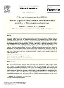
Fig. 2. Plot of fall velocity (ms ) versus diameter (mm) on November 30, 2006. Data from the freezing rain period (00-08 UTC) are in green, the mixed phase period (08-16 UTC) are in pink, and the frozen precipitation period (16-24 UTC) are in blue. Also plotted are a fourth degree polynomial approximation of the Gunn and Kinzer raindrop terminal fallspeed, a first degree polynomial approximation of the terminal fallspeed of snow, and the velocity function used to separate the rain and snow PSDs.

than most of the velocities measured by the disdrometer. The density of these particles, then, should be greater than in the Brandes relation. Ways to improve the calculation of the dielectric constant were thus considered. Given that water is present in mixed phase and wet snow particles, a Maxwell-Garnet mixture of water and snow could be used to create a more realistic dielectric constant. However, this requires knowledge of the amount of water present in a particle, which could not be gleaned from the available information. Thus, any mixture would have to be arbitrarily defined. Another alternative was to use a constant multiplicative factor to adjust the Brandes density relation. It is highly unlikely, though, that a situation would exist that would affect density in such a way. In order to create a more realistic value of density, a velocity-based modification to the density value was derived from the equation for terminal fall velocity in Pruppacher and Klett (1997). The value for ρs from (6) is recast as a baseline density, ρb, the measured velocity is represented by vm, and we use a baseline vb = 0.8467 + 0.01714D to create an estimate of ρs to replace (6):

v ρ s = ρ b  m  vb

2

  . 

(7)

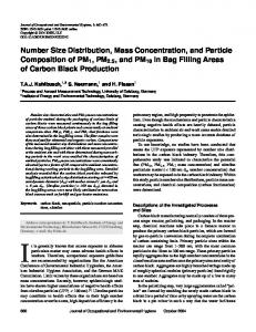
Since the particles in the snow PSD are being treated as frozen, the density is capped at 0.92 g -3 cm . Figure 3 shows the effect of this velocity adjustment on density from the November 30 event. Results for these events were calculated using both equation (6) and (7) to see how the calculation of polarimetric variables were affected by this density adjustment.

Fig. 3. Plot of density versus diameter for November 30, 2006. Also plotted is the baseline density, from Brandes et al (2007).

While looking at the disdrometer data, it became apparent that the density relation in equation 6 may not best describe the density of the snowfall during these events. Figure 2 shows a plot of measured fall velocities on November 30, 2006. The portion of primary interest are those points plotted in blue, which signify particles measured in the snow portion of the event. In addition, the fall velocity as predicted by a particle following the Brandes density relation is plotted. It becomes apparent that the expected fall velocity is lower

3.2 Using Melting Models to Create a Melted Rain DSD From Disdrometer Measurements of Snow The disdrometer collects information over oneminute intervals. However, it is sometimes preferable, particularly for stability during times of light precipitation, to find a particle size distribution over a longer period of time. The PSD can be found using the following:

N ( D) =

N T ( D) , Av( D)T

(8)

where NT(D) is the total number of drops per bin, A is the collection area, v(D) is the average drop velocity per bin, and T is the collection time. It can also be useful to fit an analytical PSD model to the measured data. Following Ulbrich (1983), a gamma distribution can be fitted to the data in the form

N ( D) = N 0 D µ exp(−ΛD)

(9),

where N0 is a number concentration parameter, µ a shape parameter, Λ a slope parameter, and D the equivolume diameter. When a distribution is predominantly composed of frozen particles, a melting model can be applied to the PSD to see how the distribution would change had it fallen through a melting layer sufficiently deep to melt all of the frozen particles. Two simple melting models were developed and applied to PSD data of frozen precipitation measured by the disdrometer. Power-law relationships are used for the density of frozen precipitation, as well as the velocity of rain. The full derivations for both melting models can be found in Appendix A. One model, which will be referred to as the “mass conservation” model, assumes that the mass of a single particle will be conserved in melting, and that the number of particles will also be conserved from frozen to liquid state. As a result, the liquid water content will be conserved from PSD to melted DSD. The melted DSD is calculated from the original PSD as

N r ( Dr ) =

N s ( Ds ) , dDr dDs

β=

N r ( Dr ) =

where

−b

The mass conservation model can also be extended to “melt” a gamma distribution fitted to the measured data, creating a new distribution of the form

N r ( Dr ) = N 0,r Drµ exp(− Λ r Drβ ) ,

(13)

where µ +1

3 − 3− b , a 3−b 3µ + b , µr = s 3−b

N 0, r = N 0 , s

Λr = a and

−

1 3− b

Λs ,

dDr d is as in (11) and cDr is a power law dDs

µ +1

1 3 − 3− b N 0, r = N 0 , s a , c 3−b 3µ + b µr = s −d, 3−b

(11)

3 − b 3− b 3 − b a Dr .(12) 15 1

dDr =

(14a) (14b) (14c)

N s ( Ds ) , (15) dDr cDrd dDs

relationship for the velocity of a rain drop. The new bin sizes are found as in (12). Like the mass conservation model, the mass and number flux conservation model can also be applied to a gamma distribution, and expressed in the same form as 13, but where

and

where a and b are coefficients of the power-law -b relationship, ρs = aDs . After melting, the uniform bin size set by the disdrometer no longer applies, and a new bin size is calculated:

(14d)

The other model, the “mass and number flux conservation” model, also assumes that the mass of a particle will be conserved. However, this model assumes that the number flux will be conserved. Unlike the mass conservation model, the liquid water content will not be conserved, but rather the snow water equivalent and rain rates will be equal. The DSD found from the original frozen PSD is calculated as

(10)

dDr 3 − b 1 / 3 −b / 3 = a Ds , dDs 3

3 . 3−b

Λr = a

−

1 3− b

Λs ,

(16a) (16b) (16c)

and

β=

3 . 3−b

(16d)

Because the relationship used for density is the Brandes power law relationship for snow, these models are only appropriate for periods of snow.

4. Data Analysis 4.1 Comparison of Z and ZDR calculated from disdrometer data and radar measurements Modeled reflectivity and differential reflectivity from the collected disdrometer data using the Brandes density relation were compared with the observations from KOUN (0.5° elevation angle) over Kessler Farm. Figure 4 shows this comparison for the November 30 event. In addition, wind speed and gusts, as well as surface temperature from the Washington site of the Oklahoma Mesonet are shown. During periods in which the precipitation was predominantly rain, the

Fig. 4. KOUN and modeled polarimetric variables from the OU 2DVD for November 30, 2006. Z is plotted in the top panel, and ZDR in the panel below that. The third panel from the top is the surface temperature as measured by the WASH mesonet site, and the bottom panel displays wind speed and gusts measured by WASH.

comparisons are favorable. However, during periods in which there was mixed phase precipitation, the disdrometer begins to show a low bias compared to the KOUN measurements. In the periods of frozen precipitation, this difference becomes very large. Fortunately, the two datasets were qualitatively similar, despite their quantitative differences.

The same comparisons between Z and ZDR are shown in Figure 5, but the values calculated from the 2DVD measurements use the velocityadjusted density for frozen precipitation. Using a more accurate estimate of density, the results show improvement, sometimes dramatically. The differences between KOUN and the 2DVD are essentially erased during the mixed phase period

Fig. 5. Comparison of Z (top panel) and ZDR (bottom panel) between KOUN and OU 2DVD on November 30 using the variable adjustment to the baseline Brandes et al density.

on November 30. 2DVD measurements are more similar to KOUN observations during the snow period on November 30, but there are still differences between the two. Both Z and ZDR are still more similar than before – for example, reflectivity differences are now only a few dB rather than more than 10. Even with the density adjustment, comparisons between disdrometer and radar measurements may be inappropriate during periods of very light snow, though. As in any other data involving radar and disdrometer data, it is important to note that the resolution volumes of the two instruments are not the same. In this case, the center of KOUN’s main lobe is about 500 meters above the disdrometer (Ryzhkov et al 2008). Thus, the two instruments are not measuring the exact same particle distributions. Particles in the KOUN resolution volume could be advected away from above the disdrometer, while some particles that fall into the disdrometer could have been in a resolution volume at radar level that was not considered. This is particularly an issue with snow, which falls much more slowly than ice pellets or rain. The resolution volume of KOUN is also considerably larger than what is measured by the disdrometer. This drop sorting is also discussed, albeit for exclusively liquid precipitation, in Lee and Zawadzki (2005). Wind effects could also be responsible for some error. Nešpor et al (2000) highlight the potential for undercatching by the disdrometer due to wind effects. That study

-1

shows that even a relatively light wind (3 ms ) can distort the flow around the sampling area of the disdrometer. The result is that a significant undercatching of particles by the disdrometer occurs. This study applied to the original design of the Joanneum Research 2DVD, which was redesigned after Nešpor et al to mitigate these problems. The OU 2DVD is one of the newer, low profile 2DVDs. While no similar studies have been done on the low profile 2DVD, it is probable that wind effects are still an issue to be considered. In addition to physical issues concerning the disdrometer, another source of error lies in the mathematical modeling of the radar variables from disdrometer data. For computational efficiency, the drops were considered to have an axis ratio of 0.7. Measurements show that this is not always the case. This would most directly affect ZDR, but could also affect Z. The ideal solution – ignoring computational concerns – would be to use the axis ratio of each particle measured by the disdrometer. Considering computational efficiency, a better solution may be to adopt the axis ratio scheme used by Ryzhkov et al (2008). 4.2 Precipitation microphysics and melting models Gamma distributions were fitted to all PSDs measured by the disdrometer during the events. Also, data during periods of only frozen precipitation had both the mass conservation and the mass and number flux conservation models applied to them. From the results, several

Fig. 6. Scatter plots of microphysical parameters from disdrometer data. The leftmost column is measured data during periods of rain. The two right columns are the results of the melting models applied to data measured during periods of snow.

characteristics were calculated, including median drop diameter, liquid water content, reflectivity, rain rate, and total number concentration. Figure 6 shows various comparisons of these parameters. The top row are D0-w scatter plots, the second row D0-Z plots, the third row NT-w plots, and the bottom row are w-R plots. Both the measured rain DSD and the results of the melting models have qualitatively similar results, but also show differences which illustrate a

need for refining the models. In the D0-w plots, there are a large cluster of small liquid water contents, with an extending branch of higher liquid water contents. However, this extending branch is much broader and occurs at a higher median diameter in the measured rain data than in either of the models. The median diameter is also smaller in the results of the mass and number flux conservation model. While the number of small drops in the melted DSDs decreases from the

snow PSD to the melted result, it does not seem to adequately match what is seen in periods of rain. The melting models do not account for collision and coalescence, which could be a factor. This factor seems to appear in the second row of plots as well; median diameter tends to increase with reflectivity but this trend is much more pronounced in the measured data than in the model results, again particularly in the mass and number flux conservation model. In the third row, this factor is seen in the large number of total drops in the melting model results compared to the periods of rain. As would be expected, the liquid water content stays very consistent in the mass conservation model, but less so in the other model. The bottom row shows a roughly linear increase in liquid water content with rain rate across the board, though the slope increases with the mass conservation model, and a bit more so with the mass and number flux conservation model. However, for smaller rain rates, the match seems closer between all three than at larger rain rates. These results show a promising match in trends between the actual rain measurements, and the resultant rain distributions from melting the snow data. At the same time, there is clearly a need to find ways to refine the models and come up with a more accurate result, particularly in their handling of small drops. The use of the Brandes density relation may be a factor as in the polarimetric variable results. The density adjustment used earlier could be helpful, but would be more difficult to bring into the model due to its dependence on drop diameter. It is important to note that a direct comparison between the periods of rain and the melted distributions from the periods of snow may not be as straightforward as would be desired. There can be significant differences in the character of precipitation as a storm evolves which make comparison between different periods more difficult. This is particularly evident in the November 30 event, as rain early in the event was associated with areas of convection, rather than stratiform precipitation. All of the snow, however, is associated with stratiform regions of precipitation. 5. Summary and Conclusions Observations of several winter precipitation events were made during 2006-2007 by the polarimetric radar KOUN and a 2D video disdrometer operated by the University of Oklahoma at the Kessler Farm Field Laboratory. The disdrometer data was used to calculate

values of Z and ZDR, which were then compared to KOUN data. The initial comparisons between the two datasets for the November 30, 2006 event showed that while the general patterns matched throughout an event, there is not very good agreement. Differences in resolution volumes, size sorting, and deformations of flow around the disdrometer could account for some of the difference between the radar and disdrometer. It was also found that the scattering amplitudes of frozen precipitation could be calculated more accurately using a variable density adjustment factor, which is determined from the fall velocities measured by the disdrometer. After recalculation of the radar variables from disdrometer data, a much better agreement – though not an exact match – was found with KOUN. Improvements can be made to the calculations. This scheme uses the density and velocities of dry snow as a baseline for all frozen precipitation. Following Yuter and creating a graupel category, and adjusting the density from a new baseline graupel density could result in improved density estimation for that type of precipitation. Also, reintroducing a water-ice mixture for partially frozen precipitation could make both the rain and snow PSD categories more realistic. However, it would be necessary to find a way to deduce the amount of water present from the disdrometer data to accomplish this task. Alternatively, given the generally good agreement found, it may be more practical to work in the reverse, and attempt to use the KOUN data to retrieve particle size distributions of transition and frozen precipitation. These retrievals could then be compared with the measured disdrometer data. Work has been done along these lines with rain drop size distributions, and should be applicable to winter precipitation. Two melting models were also applied to periods of frozen precipitation, and the results compared to periods of rain. The same trends appear in both the data from periods of rain and the results of the melting models, which is promising. Some differences could be accounted for by the changing nature of precipitation over time, particularly since some of the rain is convective, while all of the snow was stratiform. Approximations used in determining the density and particle velocity could also cause error in the model. Refining the model to account for these differences could result in more accurate results. When sufficiently accurate, there could be applications towards numerical models to improve the handling of precipitation in the presence of a melting layer.

References Brandes, E.A., K. Ikeda, G. Zhang, M. Schonhuber, R.M. Rasmussen, 2007: A Statistical and Physical Description of Hydrometeor Distributions in Colorado Snowstorms Using a Video Disdrometer. J. Appl. Meteor., 46, 634-650. Bringi, V.N., V. Chandrasekar, J. Hubbert, E. Gorgucci, W.L. Randeu, M. Schonhuber, 2003: Raindrop Size Distribution in Different Climatic Regimes from Disdrometer and Dual-Polarized Radar Analysis. J. Atmos. Sci., 60, 354-365. Bringi, V.N., M. Thurai, K. Nakagawa, G.J. Huang, T. Kobayashi, A. Adachi, H. Hanado, S. Seikizawa, 2006: Rainfall Estimation from C-Band Polarimetric Radar in Okinawa, Japan: Comparisons with 2D-Video Disdrometer and 400 MHz Wind Profiler. J. Meteor. Soc. Japan, 84, 705-724. Cao, Q., G. Zhang, E. Brandes, T. Schuur, A Ryzhkov, K. Ikeda, 2008: Analysis of video disdrometer and polarimetric radar data to characterize rain microphysics in Oklahoma. J. Appl. Meteor., in press. Chilson, P.B., G. Zhang, T. Schuur, L.M. Kanofsky, M.S. Teshiba, Q. Cao, M. Van Every, G. Ciach, 2007: Coordinated in-situ and Remote Sensing Precipitation Measurements at the Kessler Farm Field Laboratory in Central rd Oklahoma. Preprints, 33 Int. Conf. on Radar Meteorology, Cairns, Queensland, Australia, Amer. Meteor. Soc. Cortinas, J., 2000: A climatlogy of freezing rain in the Great Lakes region of North America. Mon. Wea. Rev., 128, 3574–3588. Cortinas, J.V., B.C. Bernstein, C.C. Robbins, J.W. Strapp, 2004: An Analysis of Freezing Rain, Freezing Drizzle, and Ice Pellets across the United States and Canada: 1976–90. Wea. Forecasting, 19, 377-390. Doviak, R.J. and D.S. Zrnić, 1993: Doppler Radar nd and Weather Observations. 2 Ed. Academic Press. 562 pp. Goddard, J.W.F., S.M. Cherry, V.N. Bringi, 1982: Comparison of Dual-Polarization Radar Measurements of Rain with Ground-Based Disdrometer Measurements. J. Appl. Meteor., 21, 252-256.

Henson, W., R. Stewart, B. Kochtubajda, 2007: On the precipitation and related features of the 1998 Ice Storm in the Montréal area. Atmospheric Research, 83, 36-54. Herzegh, P.H., and A. R. Jameson, 1992: Observing precipitation through dual-polarization radar measurements. Bull. Amer. Meteor. Soc., 73, 1365–1374. Ibrahim, I.A.; Chandrasekar, V.; Bringi, V.N.; Kennedy, P.C.; Schoenhuber, M.; Urban, H.E.; Randen, W.L., 1998: Simultaneous multiparameter radar and 2D-video disdrometer observations of snow. Geoscience and Remote Sensing Symposium Proceedings, IGARSS '98, pp.437439 vol.1. Ishimaru, A., 1991: Electromagnetic Wave Propagation, Radiation, and Scattering. PrenticeHall. 637 pp. Kruger, A. and W.F. Krajewski, 2002: TwoDimensional Video Disdrometer: A Description. J. Atmos. Tech., 19, 602-617. Lee, G. and I. Zawadzki, 2005: Variability of Drop Size Distributions: Noise and Noise Filtering in Disdrometric Data. J. Appl. Meteor., 44, 634-652. Loffler-Mang, M. and U. Blahak, 2001: Estimation of the Equivalent Radar Reflectivity Factor from Measured Snow Size Spectra. J. Appl. Meteor., 40, 843-849. Martner, B.E., J.B. Snider, R.J. Zamora, G.P. Byrd, T.A. Niziol, and P.I. Joe, 1993: A RemoteSensing View of a Freezing-Rain Storm. Mon. Wea. Rev., 121, 2562-2577. Nešpor, V., W.F. Krajewski, A. Kruger, 2000: Wind-Induced Error of Raindrop Size Distribution Measurement Using a Two-Dimensional Video Disdrometer. J. Atmos. Tech., 17, 1483-1492. Pruppacher, H. R., and J. D. Klett, 1997: Microphysics of Clouds and Precipitation. Kluwer Acad. 954 pp. Ryzhkov, A.V., and D.S. Zrnić, 1998: Discrimination between rain and snow with a polarimetric radar. J. Appl. Meteor., 37, 1228– 1440.

Ryzhkov, A.V., T.J. Schuur, D.W. Burgess, P.L. Heinselman, S.E. Giangrande, D.S. Zrnić, 2005: The Joint Polarization Experiment: Polarimetric Rainfall Measurements and Hydrometeor Classification. Bull. Amer. Meteor. Soc., 86, 809824. Ryzhkov, A.V., G. Zhang, S. Luchs, L. Ryzhkova, 2008: Polarimetric Characterisitics of Snow Measured by Radar and 2D Video Disdrometer. Preprints, Fifth European Conference on Radar in Meteorology and Hydrology, Helsinki, Finland. Scharfenberg, K., K. Elmore, C. Legett, T. Schuur, 2007: Analysis of Dual-Pol WSR-88D Base Data Collected During Three Significant Winter Storms. Preprints, 33rd Int. Conf. on Radar Meteorology, Cairns, Queensland, Australia, Amer. Meteor. Soc. Schönhuber, M., G. Lammer, W.L. Randeu, 2008: The 2D-Video-Distrometer. Precipitation: Advances in Measurement, Estimation and Prediction. Springer. pp. 3-31. Schuur, T., A.V. Ryzhkov, D.S. Zrnić, M. Schönhuber, 2001: Drop Size Distributions Measured by a 2D Video Disdrometer: Comparison with Dual-Polarization Radar Data. J. Appl. Meteor., 40, 1019-1034. Stewart, R. E., 1992: Precipitation types in the transition region of winter storms. Bull. Amer. Meteor. Soc., 73, 287–296. Straka, J.M., D.S. Zrnić, and A.V. Ryzhkov, 2000: Bulk Hydrometeor Classification and Quantification Using Polarimetric Radar Data:

Synthesis of Relations. J. Appl. Meteor., 39, 13411372. Thurai, M., G.J. Huang, V.N. Bringi, W.L. Randeu, M. Schonhuber, 2007: Drop Shapes, Model Comparisons, and Calculations of Polarimetric Radar Parameters in Rain. J. Atmos. Tech., 24, 1019-1032. Tokay, A., V.N. Bringi, M. Schonhuber, G.J. Huang, B. Sheppard, D. Hudak, D.B. Wolff, P.G. Bashor, W.A. Petersen, G. Skofronick-Jackson, 2007: Disdrometer Derived Z-S Relations In South Central Ontario, Canada. Preprints, 33rd Int. Conf. on Radar Meteorology, Cairns, Queensland, Australia, Amer. Meteor. Soc. Trapp, R.J., D.M. Schultz, A.V. Ryzhkov, R.L. Holle, 2001: Multiscale Structure and Evolution of an Oklahoma Winter Precipitation Event. Mon. Wea. Rev., 129, 486-501. Ulbrich, C.W., 1983: Natural Variations in the Analytical Form of the Raindrop Size Distribution. J Appl. Meteor., 22, 1764-1775 . Yuter, S.E., D.E. Kingsmill, L.B. Nance, M. LofflerMang, 2006: Observations of Precipitation Size and Fall Speed Characteristics within Coexisting Rain and Wet Snow. J. Appl. Meteor., 45, 14501464. Zerr, R., 1997: Freezing rain: An observational and theoretical study. J. Appl. Meteor., 36, 16471661. Zrnić, D.S. and A.V. Ryzhkov, 1999: Polarimetry for Weather Surveillance Radars. Bull. Amer. Meteor. Soc., 80, 389-406.