ial electronic variometer and the DI-flux, which are in use today in most magnetic observatories. The introduction of the proton preces- sion magnetometer ...
Comp. by: ASaid Maraikayar Date:23/10/06 Time:21:22:30 Stage:First Proof File Path://spiina1001z/womat/ production/PRODENV/0000000005/0000001725/0000000005/0000096473.3D Proof by: QC by:
O
OBSERVATORIES, INSTRUMENTATION
operational simplification and improvement in the measurement accuracy of the magnetic induction (see Instrumentation, history of ).
Introduction
Geomagnetic metrology
The main task of a geomagnetic observatory is to observe the natural geomagnetic field for an extended period of time (at least 1 year) by performing continuous measurements of the three-dimensional geomagnetic vector. Observatory instrumentation is responsible for this measurement task. As we are dealing with a very wide-frequency spectrum of signals, whose characteristic times extend from centuries to subsecond intervals (see Geomagnetic spectrum, temporal), issues of long-term instrument reliability, standardization of the instrumentation, continuity in data formats, as well as fast sampling capability are to be considered carefully. As only the natural geomagnetic field is of interest here, observatory instrumentation should be completely nonmagnetic: it should not modify the direction or amplitude of the geomagnetic vector in a measurable way. If, however, the sensors are magnetic, or produce magnetic fields for the sake of the measurement procedure, it must be ensured that those effects are eliminated by the measurement protocol and that no perturbation on neighboring instruments arises. For the instrumentation to perform successfully, the observatory must answer to strict magnetic conditions: low magnetic gradient and identity of field changes over the area. Moreover, one is led to consider the whole observatory site as part of the observatory instrumentation; hence the quality of measurement depends on the magnetic hygiene of the surroundings and the buildings, on low magnetic noise conditions, as well as on the stability of the pillars bearing the field orientation sensors. Detailed information about geomagnetic instrumentation in observatories can be found in Jankowski and Sucksdorff, 1996.
To completely describe the geomagnetic vector, each measurement must sample three independent vector components. The three most popular coordinate systems for describing the geomagnetic vector are: Cartesian: X (North component), Y (East component), Z (vertical component, positive downward). Cylindrical: D (magnetic declination angle, positive East), H (horizontal component), Z Spherical: D, I (magnetic inclination angle, positive downward), F (magnetic field induction intensity). Component magnetometers will measure projections of the vector with a large constant parts, like X and Z, while orientation magnetometers will be sensitive to the orientation of the field with respect to the sensor and measure small projections like D or Y. Component and orientation magnetometers are not yet capable of continuously measuring all the field components with the required absolute accuracy. Therefore, an observatory measurement setup uses:
Short history The first magnetic observatory instrument—the magnetic compass— was discovered in China already before the year A.D. 1000:. Early observatories—starting in the 16th century—used an oversize compass needle so as to ensure sufficient resolution on the declination angle. The compass was later complemented by the dip circle for measuring the magnetic inclination. Still later, projected field components would be measured by using setups with current-carrying coils and calibrated magnets. A (virtual) visit to the Museum of the History of Science in Florence will allow you to see those early instruments. Continuous observations were performed by an observer making a reading every 2 h or so and writing the values down in a notebook. The photographic paper recorder appeared in the 19th century, allowing uninterrupted graphical registration of the field. The invention of the fluxgate in the early 1900s permitted the development of the triaxial electronic variometer and the DI-flux, which are in use today in most magnetic observatories. The introduction of the proton precession magnetometer (Packard and Varian, 1954) allowed an important
� a variometer to measure the variation of the field components about
baseline values in a continuous and unattended way at the required sampling rate, say 1 Hz and � absolute measurements performed regularly (say 2 per week) by an observer with the adequate instrumentation (DI-flux, proton magnetometer; see Figure O4) to establish the values of the baselines. This makes the observatory measurement essentially a two-step process, where the second part is performed manually. Postprocessing merges the two data sets to produce a final data record having the accuracy of the absolute instruments at the variometer's sampling rate. The expression “absolute measurement" means here that the observations must be fully traceable to metrological standards for the magnetic induction and that the orientation of the geomagnetic vector is measured with respect to the local vertical and to geographic north. It is expected that in the future fully automatic observatories will be available (see Observatories, automation) where the absolute measurement part will be also unattended. Observers are striving to make absolute measurements with an accuracy of 0.1 nT for inductions and 1 s of arc for orientation. The INTERMAGNET consortium (see Observatories, INTERMAGNET) has laid down observatory instrumentation specifications for its members. This conveniently provides guidelines for observatories wishing to upgrade their instrumentation. In less-modern observatories, variometers consist of suspended magnets and magnetic balances (Wienert, 1970). The continuous record of the field's components is recorded as curves on a piece of photographic paper, the magnetogram. Elongated axial magnets, suspended so as to rotate freely around the vertical, will orient their magnetic axis along the geomagnetic meridian, and will thus indicate its direction, providing a declination variometer. If an auxiliary stationary magnet creates a bias field so as to position the suspended magnet with
Comp. by: ASaid Maraikayar Date:23/10/06 Time:21:22:31 Stage:First Proof File Path://spiina1001z/womat/ production/PRODENV/0000000005/0000001725/0000000005/0000096473.3D Proof by: QC by:
2
OBSERVATORIES, INSTRUMENTATION
Modern proton magnetometers can be quite compact and have high resolution and sampling rate (0.01 nT and 3 Hz are typical). The Overhauser types (Sapunov et al., 2001) in particular are responsible for this progress and have the additional benefit of low power operation. They are therefore a first choice in modern observatories instrumentation, providing automatic and continuous observation of the geomagnetic induction field intensity.
The optically pumped magnetometer
Figure O4 Instrumentation as used in most magnetic observatories of the world. The left panel represents a triaxial fluxgate variometer sensor. Right panel: the DI-flux magnetometer mounted on top of the pillar consists of a nonmagnetic theodolite with a fluxgate sensor on its telescope. In the foreground, an Overhauser proton magnetometer consisting of the cylindrical sensor and the electronic console.
its magnetic axis east–west, the suspended magnet's motion will follow the changes in the horizontal component, allowing it to be recorded. Magnetic balances compare the torque exerted by the vertical component on a magnet with the one exerted by gravity on a constant mass using a knife-edge balance. In all cases, the recording of the magnet's motion is ensured by a light beam falling on a mirror at the magnet's extremity. The horizontal beam, deflected by this mirror, will impress a time-dependent curve on a vertically streaming photographic paper. The streaming speed is usually about 20 mm h�1, but for rapid run magnetographs it may go up to 200 mm h�1. In modern observatories, the most popular magnetometers are based on the proton precession effect and the fluxgate sensor. In former Soviet bloc countries, the Bobrov magnetometer, which consists of a magnet suspended by a taut quartz fiber, is successfully used in its servo version, where the magnet's orientation is kept fixed by the action of a coil. The coil current is easily fed to a digital data acquisition system to produce computer readable files.
It is used in observatories for measuring the magnetic induction B in the range of 10–100 mT with accuracy down to 0.1 nT. Here the free precession frequency f of protons is the observable and the formula (Eq. 1)
allows the measurement of the magnetic induction by way of the measurement of a frequency. The standard for the magnetic induction is thus conveniently converted to a frequency standard, which is widely available. The quantity � 0 p is the proton gyromagnetic ratio at low field for a spherical H2O sample at 25 � C. The recommended value given by CODATA and adopted by IAGA in 1992 is (Cohen and Taylor, 1987) � 0 p ¼ 2:67515255T�1 s�1
Induction coil magnetometer The induction coil (or search-coil) magnetometer's (ICM) operation principle is based on the Maxwell equation which can be written in integral form as e¼�
The proton precession magnetometer
2�f ¼ � 0 pB
Optically pumped magnetometers (OPM) are based on the splitting of the energy levels of some alkali metal and helium atoms in a magnetic field. The optical pumping scheme allows measuring this energy splitting with very high resolution (Alexandrov and Bonch-Bruevich, 1992). OPMs have been used at magnetic observatories, both for total field modulus measurement and, when complemented by a set of bias coils, for observing the geomagnetic field direction changes. One of the first digital observatories was based on a rubidium OPM (Alldredge and Saldukas, 1964). Like proton magnetometers, the OPMs are scalar magnetometers but, to the contrary of the proton magnetometer, deliver a continuous stream of data, in the form of a frequency modulated by the value of the field. This frequency, with name of Zeeman, is linked to the measured magnetic induction by the Breit–Rabi polynomial formula. In a few cases, when the Zeeman peaks corresponding to the different energy-splits in the atoms are resolved, the polynomial coefficients can be calculated from fundamental physical constants, and the OPM has then absolute accuracy. This is the case of the OPMs based on potassium, 3He, and 4He vapor (Alexandrov and Bonch-Bruevich, 1992; Gilles et al., 2001). OPMs have a high sensitivity with some approaching the 0.1 pT Hz�1/2 noise level. This performance makes them attractive for prospection work, aeromagnetic survey, space-based observations, and field stabilizers. However their high initial and maintenance cost due to the short lifetime of the gas-discharge pumping lamp has limited their use in the observatory. It looks like this deficiency will be overcome in the future in view of quick progress in laser-pumping lamps (Gilles et al., 2001).
(Eq. 2)
The sensor consists of a bottle containing the proton-rich fluid and is surrounded by a coil, serving the dual purpose of applying periodically a polarizing field to the liquid and picking up the signal from the precessing protons after cutting off the polarizing field. An electronic console will amplify the precession signal and perform a frequency measurement of it with the required accuracy. This measurement is then scaled using � 0 pto give the field induction intensity in teslas. This quite remarkable instrument is one of the few sensors able to measure directly the modulus of a vector without using computation from components or performing a leveling or tedious orientation procedure. This is of course due to the fact that the free protons have only the ambient magnetic field to orient themselves.
d� ; dt
where e is the electromotive force (emf ), F is the magnetic flux, and t is the time. In its simplest form an ICM contains a coil with many turns of copper wire connected to the input of a voltage amplifier. As it is seen from the equation, an ICM can be used only for the measurement of a time-varying magnetic flux. Its component collinear to the coil's axis intercepts the coil loops and generates an emf at the coil's terminals, which is further amplified to an easily measurable level. To increase the ICM sensitivity, a high permeability ferromagnetic material is used as a core inside the multiturn winding. Due to their relative simplicity, ICMs are widely used for many applications, mainly in geophysics. In geomagnetic observatories they are used for the study of Earth's magnetic field pulsations. Their operational frequency band covers from about 10–4 till 10þ7 Hz and the measurement dynamic range covers the range from fractions of femtotesla till tens of tesla. In spite of an apparent simplicity, the creation of a high-class ICM needs complicated calculations to establish an optimal matching of the sensor coil with the amplifier (Korepanov et al., 2001).
The fluxgate magnetometer This instrument is used for measuring the component of the magnetic field vector along its sensor's axis. The fluxgate principle uses the nonlinear field/induction relationship of an easily saturable ferromagnetic core. The core, usually a rod or a ring, is subjected to both the DC field to be measured, and an auxiliary AC field produced by a coil and an electronic oscillator. This offset sinusoidal excitation will create
Comp. by: ASaid Maraikayar Date:23/10/06 Time:21:22:33 Stage:First Proof File Path://spiina1001z/womat/ production/PRODENV/0000000005/0000001725/0000000005/0000096473.3D Proof by: QC by:
OBSERVATORIES, INSTRUMENTATION
a distorted AC signal, in a pick-up coil surrounding the core. The detection of its even harmonics provides a DC signal proportional to the field to be measured. Fluxgate sensors work best in small axial fields, therefore they are often operated within a third current-carrying coil, which cancels off the main part of the DC field. This main part may be calculated by a servo scheme, or be constant. Otherwise, the fluxgate sensor is operated with the field essentially normal to the sensor, resulting in a small field component along the core axis. The fluxgate will then be sensitive to its orientation to the field. Observatory fluxgate variometers will include three fluxgate sensors arranged orthogonally on a stable support made of marble or quartz. This trihedron is then oriented by the variometer frame according to the three components set if one wishes to observe (see Figure O4).
Absolute measurements of declination and inclination Measuring the orientation of the geomagnetic vector with respect to a coordinate frame pointing to the geographic north and to the local vertical represents a metrological challenge, especially if one wishes to attain 100 direction accuracy on this fluctuating vector. In fact, several measurements are taken so as to correct for systematic instrumental defects. Therefore the variometer of the observatory is used for taking into account any field changes during the measurement procedure. The state of the instrumentation art is now provided by a device called “DIflux" or “DIM," which is assembled from a nonmagnetic theodolite and a fluxgate sensor mounted on the telescope. The magnetic axis of the fluxgate should be nearly parallel to the optical axis of the telescope (see Figure O4). With a DI-flux so configured, a measurement protocol suggested by Lauridsen (1985) allows the error-free determination of D and I. Jean L. Rasson
Bibliography Alldredge, L.R., and Saldukas, I., 1964. An automatic standard magnetic observatory. Journal of Geophysical Research, 69: 1963– 1970.
3
Alexandrov, E.B., and Bonch-Bruevich, V.A., 1992. Optically pumped magnetometers after three decades. Optical Engineering, 31: 711–717. Cohen, E.R., and Taylor, B.N., 1987. The 1986 CODATA recommended values of the fundamental physical constants. Journal of Research of the National Bureau of Standards (U.S.), 92: 85–95. Gilles, H., Hamel, J., and Chéron, B., 2001. Laser pumped 4He magnetometer. Review of Scientific Instruments, 72: 2253–2260. Jankowski, J., and Sucksdorff, C., 1996. Guide for Magnetic Measurements and Observatory Practice. Boulder: International Association of Geomagnetism and Aeronomy. Korepanov, V., Berkman, R., Rakhlin, L., Klymovych, Ye., Pristai, A., Marussenkov, A., and Afanassenko, M., 2001. Advanced field magnetometers comparative study. Measurement, 29: 137–146. Lauridsen, K.E., 1985. Experiences with the DI-fluxgate magnetometer inclusive theory of the instrument and comparison with other methods. Danish Meteorological Institute Geophysical Papers, R-71. Packard, M., and Varian, R., 1954. Physical Review, 93: 941. Sapunov, V., Denisov, A., Denisova, O., and Saveliev, D., 2001. Proton and Overhauser magnetometers metrology. Contributions to Geophysics & Geodesy, 31: 119–124. Wienert, K.A., 1970. Notes on Geomagnetic Observatory and Survey Practice. Brussels: UNESCO.
Cross-references Compass Gauss’ Determination of Absolute Intensity Geomagnetic Spectrum, Temporal Instrumentation, History of Magnetometers, Laboratory Observatories, Automation Observatories, INTERMAGNET
Au1
Comp. by: ASaid Maraikayar Date:23/10/06 Time:21:22:34 Stage:First Proof File Path://spiina1001z/womat/ production/PRODENV/0000000005/0000001725/0000000005/0000096473.3D Proof by: QC by:
Author Query Form Title: Encyclopedia of Geomagnetism and Paleomagnetism Alpha - O
__________________________________________________________________________ Query Refs.
Details Required
AU1
Kindly provide the article title for the reference “Packard and Varian, 1954.”
Author’s response