Obstacle Avoidance in Collective Robotic Search Using Particle Swarm Optimization Lisa L. Smith, Student Member, IEEE, Ganesh K. Venayagamoorthy, Senior Member, IEEE, Phillip G. Holloway Real-Time Power and Intelligent Systems Laboratory University of Missouri-Rolla, MO 65409-0249, U.S.A.
[email protected],
[email protected],
[email protected]
Abstract – Particle Swarm Optimization (PSO) has been demonstrated to be a useful technique in target search applications such as Collective Robotic Search (CRS). A group of unmanned mobile robots are able to locate a specified target in a high risk environment with extreme efficiency when driven by an optimized PSO algorithm. This paper presents an algorithm for obstacle avoidance with the PSO approach applied to navigate robots in collective search applications. Obstacles represented by basic geometric shapes to simulate perilous ground terrain are introduced to the search area. Results are presented to show that PSO algorithm based CRS is able to locate targets avoiding hazardous pathways.
I. INTRODUCTION The idea of using mobile robots for hazardous target search applications with little to no human intervention can be realized with Particle Swarm Optimization (PSO). This concept is still restricted to simulation though, since there are multiple real-world factors that limit conventional programming. Introducing obstacles into the search area and finding an efficient way for the particles to avoid them is the next big step towards real-world success. Particle swarm optimization has shown to be an effective tool for potential applications to the Collective Robotic Search (CRS) problem [1]-[2]. The main benefit of PSO is that instead of reproducing individuals to gain better overall fitness as in evolutionary algorithms, it evolves better solutions through the collective interaction of all the individuals. The group’s success is determined by the social interactions between individual members of the swarm. This allows the swarm to arrive at the best solution through systematic exploration and exploitation of the search space. The focus of this paper is to simulate ground terrain such as buildings, lakes, rivers, and mountains that will require the robots’ to navigate around these obstacles and avoid collision [3]. The PSO algorithm can be easily modified in order to allow the particles/robots to successfully consider the risks of the environment and avoid possible barriers while still continuing on an efficient trajectory leading towards total swarm convergence on the target. This paper presents modification to the collective robotic search using PSO presented in [1] to now include obstacles in the search space. The rest of the paper is organized as follows: Section II describes collective robotic search. Section III gives a brief description of particle swarm optimization as applied to CRS. Section IV presents the details of the CRS simulation with and without PSO algorithm’s ability to avoid obstacles. Section V presents some results and discussion on how the
obstacle shape and PSO parameters affect the algorithm. Finally, the conclusion and future work is given in section VI. II. COLLECTIVE ROBOTIC SEARCH A swarm of intelligent mobile robots are desirable for target search applications mainly because they remove the need for human intervention in inhospitable areas. A team of small, inexpensive, and dispensable robots can be utilized for hazardous tasks such as landmine detection, fire fighting, military surveillance, etc at less overall expense [4]. The advantage of using the PSO approach is that the number of robots is large, accommodating for the failure or destruction of a few robots without compromising the end goal [1], [5]. In the current target search algorithm, a number of robots/particles are randomly dropped into a specified area and flown through the search space with one new position calculated for each particle per iteration. The coordinates of the target are known and the robots use a fitness function, in this case the Euclidean distance of the individual robots relative to the target, to analyze the status of their current position. Just as the target coordinates are known so are the obstacle’s boundary coordinates in the simulation studies. In a real situation, the mobile robots will be equipped with sensors to measure intensities and proximities. If a particle’s next prospective position resides inside the obstacle space, an arc function is accessed in order to ‘swing’ the particle around the nearest corner of the obstacle instead of traveling straight through the obstacle resulting in a collision. As they search the area using PSO, they use their personal best position, pid, and global best position, pgd to keep them on a route leading to the target. Basic geometry tools and the Pythagorean theorem are used to analyze a particle’s current position relative to the obstacle for simulation purposes. In a real world trial, the particle’s position relative to the target or the obstacle will be determined using sensor data. III. PARTICLE SWARM OPTIMIZATION FOR CRS The basic PSO algorithm is slightly modified to accommodate for the obstacle avoidance and collective robotic search applications. As in general PSO, the robots navigate through the search space with a random velocity while storing their personal previous best position (pid) and the best position of the entire swarm relative to the target, know as the global best position (pgd). As one robot finds an optimal solution, other robots migrate towards it, in effect exploiting and exploring the best sections of the search space [6]-[7].
this figure that two robots collide with the obstacle and will not converge to the target.
The PSO-CRS algorithm can be summarized in the following steps: (i). A population of robots is initialized in the search environment containing a target and an obstacle, with random positions, velocities, personal best positions (pid), and global best position (pgd). (ii). The fitness value—Euclidean distance from the robot to the target, shown in (1)—is determined for each robot where Tx and Ty are the targets coordinates and Px and Py are the current coordinates of the individual robot. fitness =
(Tx − Px ) + (Ty − Py ) 2
xid ( k + 1 ) = xid ( k ) + vid ( k + 1 )
♦
(3)
(iv). If the next possible position xid(k+1) resides within the obstacle space, the obstacle avoidance part of the algorithm explained in Section IV is employed, otherwise the robot moves to this new position and step (v) is implemented. (v). The pid with the best fitness for the entire swarm is determined and the global best coordinate location, pgd, is updated with this pid. (vi). Until convergence is reached, repeat steps (ii) – (v).
Obstacle
♦
Robots
(1)
vid (k + 1) = w × vid (k ) + c1 × rand ( ) × ( pid (k ) − xid (k )) + (2) c2 × Rand ( ) × ( pgd (k ) − xid (k ))
♦
♦
2
(iii). The robot’s fitness is compared with its previous best fitness (pid) for every iteration to determine the next possible coordinate position for each robot in the search environment. The next possible velocity and position of each robot are determined according to (2) and (3) where vid(k+1) and xid(k+1) represent the velocity and position of the robot i at instant k+1.
♦
♦
♦
●
♦ Target
♦
♦
Fig. 1. Robots’ starting locations, square obstacle and target shown.
♦
♦
♦
♦ ♦ ♦
♦
♦
● ♦
♦
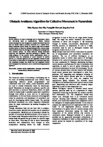
IV. CRS SIMULATION For each simulation, the search space is set to 20 by 20 units with the center point being the coordinate (0, 0). The maximum velocity (Vmax) is limited to 0.5 units. The initial positions for the robots/particles are randomly generated but limited to the boundaries of the search space and if a robot’s starting location falls with an obstacle boundary, it is reassigned to a random position outside of the obstacle. For the CRS search in this paper, 10 robots are used to search a single target. A. PSO Algorithm without Modification for Obstacle Avoidance Fig. 1 shows the starting positions of the 10 robots, a square obstacle and a target (circle). Fig. 2 shows the paths taken by the individual robots to converge at the target using the standard PSO algorithm presented in [2]. It is clear from
Fig. 2. Robots’ pathways to the target location. Two robots collide into the obstacle.
B. PSO Algorithm with Modification for Obstacle Avoidance As the particles move through the search space, gaining one new position for every iteration, a conditional statement checks to see if the next position of the particle will fall within the boundaries of the obstacle. If this condition is true, the obstacle avoidance section of the algorithm is initiated. First the nearest corner of the obstacle is calculated by measuring the Euclidean distance of the particle’s current position relative to each obstacle corner and choosing the corner with the smallest value. Then the arc function is accessed in order to ‘swing’ the particle around the nearest obstacle corner. The current coordinates of the particle are passed into the arc function as (x_start, y_start) in (4); this
will be the starting point of the 180 degree arc. The center of the arc, (x_center, y_center) in (4), is the coordinates of the nearest obstacle corner relative to the particle. The radius of the arc is set as the distance from the particle’s position to the obstacle corner that is designated as the center of the arc.
Target Obstacle
( horiz,vert,next ) = (4) arc ( x _ start, y _ start,x _ center, y _ center,dir, po int s ) The arc can either rotate in a clockwise or counter clockwise direction to maneuver around the obstacle. Also the number of points which make up the arc can be specified to control the angle that the particle will travel when moving away from the obstacle. Choosing the number of points is especially important when the obstacle occupies a large portion of the search area. If the number of points is too large, like 50 points, the angle of deflection will be extremely acute and the robots will become trapped on one side of the obstacle and unable to maneuver around it. Four arc points are used in the simulations shown in this paper. The new position of the particle is set at the second point in the arc. The second point is chosen to keep the arc function from putting the particle back into the obstacle, or from interfering with the influence of PSO on the particle’s trajectory for longer than necessary. Figure 3 illustrates graphical the arc function.
♦ ♦ ♦
Robots
♦
♦
♦
Fig. 4. Robots’ starting locations, square obstacle and target shown.
● ♦
♦
♦
♦
♦
♦ ♦
♦ Robot Position
♦
♦
♦
♦
Next Position
●
♦ ♦
♦
♦
Obstacle Corner – Center Point Fig. 5. Robots’ pathways to the target location.
Figs. 6 and 7 demonstrate the simulation of the PSO-CRS algorithm with obstacle avoidance code for a circular obstacle with radius of 2 units. The particle’s trajectories are represented by lines for a better visualization of the particle’s paths. Fig. 3. Arc function.
Figs. 4 to 7 show the starting locations of the robots and the pathways taken to converge at the target locations. PSOCRS obstacle avoidance algorithm is used to navigate around square and circular shapes obstacles. Figs. 4 and 5 demonstrate the simulation of PSO-CRS algorithm with the particle’s consideration of the ground terrain hazards as it navigates through the search space. The first obstacle is represented by a simple 2 by 2 unit square. The robots’ paths are traced by a dotted line with each dot representing one iteration’s position.
TABLE I AVERAGE NUMBER OF ITERATIONS TAKEN BY THE SWARM WITH STANDARD DEVIATIONS
Robots
♦ ♦ ♦
Obstacle Type
Obstacle
♦
Square
♦ Target
♦
●
♦ ♦
♦
♦
Circle
Over 20 Trials PSO Parameters 1 c1=0.5 c2=2, w=0.6 Average ± std 89.43 ± 9.86 Maximum
104
PSO Parameters 2 c1=2 c2=2, w=0.6 105.6 ± 10.68 128
Minimum
66
85
Average ± std
76.75 ± 8.75
106.1 ± 11.61
Maximum
95
128
Minimum
64
78
Table II compares the average number of iterations taken for convergence on the target by each robot, with square and circular obstacles in the search space, for different values of PSO parameters.
Fig. 6. Robots’ starting locations, circular obstacle and target shown.
TABLE II AVERAGE NUMBER OF ITERATIONS TAKEN BY INDIVIDUAL ROBOTS WITH STANDARD DEVIATIONS
♦ ♦ ♦
Obstacle Type
♦
♦ ♦
♦
●
♦ ♦
Square
♦
Fig. 7. Robots’ pathways to the target location.
V. RESULTS AND DISCUSSION PSO based CRS data is taken to compare how differently shaped obstacles and the value of the PSO parameter c1 affect the search process. In all of the following tests, the circle and square obstacles are centered at the origin of the search space and had a diameter/length of 2 units. The target is placed at the coordinate location (5, 5). PSO parameters c2 and w are kept at values of 2 and 0.6, respectively. The CRS is carried out for 20 trials. Table I compares the average number of iterations taken for the entire swarm of robots to collectively converge on the target for environments with square and circular obstacles for different values of PSO parameters.
Circle
Over 20 Trials PSO Parameters 1 Robot # c1=0.5 c2=2, w=0.6
PSO Parameters 2 c1=2 c2=2, w=0.6
Robot 1
92.4 ± 10.57
105.3 ± 17.99
Robot 2
84.15 ± 21.98
107.3 ± 19.52
Robot 3
89.1 ± 10.67
103.35 ± 17.84
Robot 4
89.2 ± 9.65
105.9 ± 26.28
Robot 5
90.5 ± 8.63
102.05 ± 15.56
Robot 6
91.85 ± 11
107.35 ± 16.23
Robot 7
89.4 ± 11.55
101.9 ± 11.47
Robot 8
87.05 ± 13.18
110.4 ± 17.58
Robot 9
89.4 ± 12.18
104 ± 18.89
Robot 10
91.7 ± 12.13
107.5 ± 17.92
Robot 1
78.2 ± 12.13
105.5 ± 22.24
Robot 2
74.6 ± 13.64
107.6 ± 20.41
Robot 3
75.5 ± 12.01
107.65 ± 15.54
Robot 4
79.45 ± 11.58
109.9 ± 24.75
Robot 5
75.65 ± 12.42
103.8 ± 27.55
Robot 6
82.1 ±13.27
103.45 ± 22.84
Robot 7
70.25 ± 11.01
106.78 ± 15.77
Robot 8
79.15 ±9.94
98.9 ± 19.23
Robot 9
77.45 ± 11.29
103.55 ± 24.58
Robot 10
75 ± 10.62
114.05 ± 28.78
The results from either Table I or II clearly show that a value of 0.5 for c1 produces faster convergence for the robots individually and as a swarm. These results also imply that it was easier for the robots to maneuver around the circular obstacle rather than the square. The number of iterations given in Table II per robot for the case where c1 was 0.5 is obviously smaller for the circle than the square to a degree
worth noting. One possible explanation for this is to examine the very shape of the obstacle and note that there are no obtuse corners for the circle, so the robot can follow a straighter and shorter path towards the target while traversing around the circle obstacle; the robot would need to take a more elongated route to keep from hitting the corners of the square. VI. CONCLUSION This paper has presented a successful modification to a PSO-CRS algorithm reported earlier by one of the authors to now include obstacle avoidance. The results of this paper show that applying particle swarm optimization to a collective robotic search problem is still practical and efficient for search areas with variable topography as it was for areas without. Future work will include testing the use of reinforcement learning as a means of obstacle avoidance. In addition, simulation with more realistic ground terrains such as mountains and rivers with bridges that must be crossed in order to reach the target will be considered. REFERENCES [1]. S. Doctor, G. K. Venayagamoorthy and V. Gudise, “Optimal PSO for Collective Robotic Search Applications,” IEEE Congress on Evolutionary Computations, June 19-23, 2004, Portland OR, USA, pp. 1390 – 1395. [2]. E. P. Dadios and O. A. Maravillas Jr. “Cooperative mobile robots with obstacle and collision avoidance using fuzzy logic” Proceedings of the 2002 IEEE International Symposium on Intelligent Control, 27-30 Oct. 2002, pp.75 – 80. [3]. S. Doctor, G.K. Venayagamoorthy, "Unmanned Vehicle Navigation Using Swarm Intelligence", International Conference on Intelligent Sensing and Information Processing, Chennai, India, January 4 - 7, 2004, pp. 249 - 253. [4]. M. Haenggi, “Mobile sensor-actuator networks: opportunities and challenges”, Proceedings of the 2002 7th IEEE International Workshop on Cellular Neural Networks and their Applications, 22-24 July 2002, pp. 283 – 290. [5]. N.V. Kulkarni, K. Krishna Kumar, “Intelligent engine control using an adaptive critic”, IEEE Transactions on Control Systems Technology, Volume 11, Issue: 2, March 2003, pp: 164 – 173. [6]. J. Kennedy and R. Eberhart, “Particle swarm optimization,” Proceedings, IEEE International Conference on Neural Networks, vol. 4, pp. 1942 – 1948. [7]. J. Kennedy, R. Eberhart and Y. Shi, Swarm Intelligence, Morgan Kaufman Publishers, 2001.