Email: {zengshuq, weng }@cse.msu.edu ... To greatly reduce the number of training samples ... online training was used so that the trainer could dynamically.
Proceedings of the 2004 IEEE International Conference on Robotics & Automation New Orleans, LA • April 2004
Obstacle Avoidance through Incremental Learning with Attention Selection Shuqing Zeng and Juyang Weng Department of Computer Science and Engineering Michigan State University East Lansing, Michigan 48824–1226 Email: {zengshuq, weng }@cse.msu.edu Abstract— This paper presents a learning-based approach to the task of generating local reactive obstacle avoidance. The learning is performed online in real-time by a mobile robot. The robot operated in an unknown bounded 2-D environment populated by static or moving obstacles (with slow speeds) of arbitrary shape. The sensory perception was based on a laser range finder. To greatly reduce the number of training samples needed, an attentional mechanism was used. An efficient, realtime implementation of the approach had been tested, demonstrating smooth obstacle-avoidance behaviors in a corridor with a crowd of moving students as well as static obstacles.
I. I NTRODUCTION The problem of range-based obstacle avoidance has been studied by many researchers. Various reported methods fall into two categories: path planning approaches and local reactive approaches. Path planning approaches are conducted offline in a known environment. In [1], an artificial potential field is used to find a collision-free path in a 3-D space. Such methods can handle long-term path planning but are computationally expensive for real-time obstacle avoidance in dynamic environment (moving obstacles). The local reactive approaches are efficient in unknown or partially unknown dynamic environments since they reduce the problem’s complexity by computing short-term actions based on current local sensing. The dynamic window (DW) approach [2] formulates obstacle avoidance as a constrained optimization problem in a 2-D velocity space. They assume that the robot moves in circular paths. Obstacles and the robot’s dynamics are considered by restricting the search space to a set of admissible velocities. Although they are suited for high velocities (e.g., 95cm/s), the local minima problem exists [3]. A major challenge of scene-based behavior generation is the complexity of the scene. Human expert knowledge has been used to design rules that produce behaviors using prespecified features. In [4], a fuzzy logic control approaches is used to incorporate human expert knowledge for realizing obstacle avoidance behaviors. One difficulty of a pure fuzzy approach is to obtain the fuzzy rules and membership functions. Neuro-fuzzy approach [5] is introduced with the purpose of generating the fuzzy rules and the membership functions automatically. Their training processes are usually conducted using a human supplied training data set (e.g., trajectories) in
0-7803-8232-3/04/$17.00 ©2004 IEEE
an off-line fashion, and the dimensionality of the input variable (features) must be low to be manageable. In contrast with the above efforts that concentrate on behavior generation without requiring sophisticated perception, a series of research deals with perception-guided behaviors. Studies for perception-guided behaviors have had a long history. Usually human programmers define features (e.g., edges, colors, tones, etc.) or environmental models [6]. An important direction of research, the appearance-based method [7], aims at reducing or avoiding those human-defined features for better adaptation of unknown scenes. The need to process high dimensional sensory vector inputs in appearance-based methods brings out a sharp difference between behavior modeling and perceptual modeling: the effectors of a robot are known with the former, but the sensory space is extremely complex and unknown with the latter and, therefore, very challenging. In this paper, we present an approach of developing a local obstacle avoidance behavior by a mobile humanoid through online real-time incremental learning. A major distinction of the approach is that we used the appearance-based approach for range-map learning, rather than an environmentdependent algorithm (e.g., obstacle segmentation and classification) for obstacle avoidance. The new appearance-based learning method was able to distinguish small range map differences that are critical in altering the navigation behavior (e.g., passable and not passable sections). In principle, the appearance-based method is complete in the sense that it is able to learn any complex function that maps from the rangemap space to the behavior space. This also implies that the number of training samples that are required to approximate the complex function is very large. To reduce the number of training samples required, we introduced the attentional selective mechanism which dynamically selected regions in near approximity for analysis and treated other regions as negligible for the purpose of local object avoidance. Further, online training was used so that the trainer could dynamically choose the training scenarios according to the system’s current strengths and weakness, further reducing the time and samples of training. The remainder of this paper is organized as follows. Section II presents the proposed algorithm. The robotic platform and the real-time online learning procedure are described in Section III. The results of simulation and real robot experi-
115
z(t)
x(t)
Attention
y(t+1)
IHDR v(t)
D
r(t)
f r(t)
Mobile Robot
z(t)
Fig. 2. The attentional signal generator f and attentional executor g.
r(t) and z(t) denote the input and output, respectively.
v(t+1)
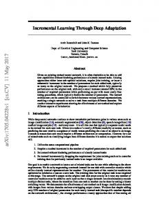
Fig. 1. The control architecture of the range-based navigation. “Attention” denotes an attentional module. rp (t) denotes the retrieved range prototype.
ments are reported in Section IV. Discussions and concluding remarks are given in Section V. II. A PPROACH A. Problem statement We formulate the obstacle avoidance behavior as a direct mapping from the current range image to action. The robot does not sense and store scene configuration (e.g., global map of the environment) nor the global position. In fact, it uses the real world as its major representation. In the work presented here, the robot’s only goal is to move safely according to the scene: It has no target location. Such a navigation system is useful for applications where a human guides global motion but local motion is autonomous. Formally, let vectors r(t) ∈ Rn and v(t) denote, respectively, the image of range scanner and the readings of encoders at time t. r(t) is a vector of distance, whose ith component ri denotes the distance to the nearest obstacle at a specific angle. The vectors r(t) and v(t) are given by two sensors whose dimension and scale are different. In order to merge them together as the single vector x(t), the following normalization is needed: r(t) − ¯r v(t) − ¯v , ), (1) x(t) = ( wr wv where wr and wv are two positive numbers that denote the scatter measurements1 of the variates r and v, respectively; and ¯r and ¯v are sample means. The obstacle avoidance behavior can be formulated as: y(t + 1) = f (x(t)).
g
(2)
where y(t + 1) denotes the action sent to the effectors. Fig. 1 shows the coarse control architecture of the presented approach. An Incremental Hierarchical Discriminating Regression (IHDR) [9] tree is generated to estimate the control signal y from x. The current input range image r(t) and the vehicle’s velocities v(t) are used for deriving the next control signal y(t + 1). An attentional module is added to extract partial views from a whole view of a scan. 1 For simplicity, we assume the covariance matrix (Σ ) of a variate u is u equal to σ 2 I, where √ I denotes √ an identical matrix. Thus, its corresponding scatter is wu = trΣu = nσ, where n denotes the dimension of the variate u (see [8] page 13).
B. Attentional mechanism Direct use an image as a long vector for statistical feature derivation and learning is called the appearance-based approach in the computer vision community. Usually the appearance-based approach uses monolithic views where the entire range data (or visual image) frame is treated as a single entity. However, the importance of signal components is not uniform. There are cases where appearances of two scenes are quite similar globally, but different actions are required. Further, similar actions are needed where the appearance of two scenes look quite different globally. Both cases indicate that there are critical areas where differences critically determine the action needed. This necessitates an attentional mechanism to select such critical areas. Definition 1: The operation of the attentional effector a(t) for input r(t) and output z(t) is defined by: � r(t) a(t) = 1, z(t) = g(r(t), a(t)) = (3) r¯ a(t) = 0, where r¯ denotes the sample mean of the raw signal r(t). For intended application, we would like to have a(t) to behave in the following way. First, when all input components have large values, the attention selection is in its default mode, turning on all components. Second, when there are nearby objects, the attention selection activates only nearby objects which are critical for object avoidance while far-away objects are replaced by their mean readings. This attentional action, as shown in Fig. 2, can be realized by two programmed functions g and f : (4) zi (t) = g(ri (t), ai (t)) and ai (t) = f (r(t)) =
�
1 if ri < T or ∀j rj (t) ≥ T, 0 otherwise,
(5)
where T is a threshold, i = 1, 2, ..., n, and r(t) = (r1 (t), r2 (t), ..., rn (t)) denotes the input vector. The above function f will suppress some far-away components (ai (t) = 0) if there are objects closer than T . If all readings are faraway, we do not want to turn the attention off completely and, therefore, we leave all attentional effectors on (∀j, aj (t) = 1). This is needed for the robot to pass through tight areas, where a small change in the width of a gap determines whether the robot can pass. Attention enables the robot to focus on critical areas and, thus, the learned behaviors sensitively depend on the attended part of the range map. In Fig. 1, the learner IHDR is a hierarchical organized high-dimensional regression algorithm. In order to develop
116
stable collision-avoidance behaviors, the robot needs sufficient training sample. [10] shows that the attentional mechanism greatly reduces the number of necessary training samples for collision avoidance.
1
20
17
Virtual label 14
7 19 8
8
14
11
23
21
3 22
5
5
2
4
12
2 18 23 4 9 15
Virtual label
18 9
13
10
C. IHDR: Memory associative mapping engine In the context of the appearance-based approach, the mapping (e.g., f in Eq. (2)) from high dimensional sensory input space X into action space Y remains a nontrivial problem in machine learning, particularly in incremental and realtime formulations. By surveying the literature of the function approximation with high dimensional input data, one can identify two classes of approaches: (1) approaches fit global models, typically by approximating a predefined parametrical model using a pre-collected training data set, and (2) approaches fit local models, usually by using temporal-spatially localized simple (therefore computationally efficient) models and growing the complexity automatically (e.g., the number of local models and the hierarchical structure of local models) to account for the nonlinearity and the complexity of the problem. The literature in the function approximation area concentrates primarily on the methods of fitting global models. For example, Multiple Layer Perceptron (MLP) [11], Radial Basis Function (RBF) [12], and Support Vector Machine based Kernel Regression methods (SVMKR) [13] employ global optimization criteria. In spite of their theoretic background, they are not suitable for the online real-time learning in highdimensional spaces. First, they require a priori task-specified knowledge to select right topological structure and parameters. Their convergent properties are sensitive to the initialization biases. Second, some of these methods are designed primarily for batch data learning and are not easy to adapt for incrementally arrived data. Third, their fixed network topological structures eliminates the possibility to learn increasingly complicated scenes. In contrast to the global learning methods described above, local model learning approaches are more suited for incremental and real-time learning, especially in the problem of a robot in an uncertain scene. Since there is limited knowledge about the scene, the robot, itself, needs to develop the representation of the scene in a generative and data driven fashion. Typically the local analysis (e.g., IHDR [9] and LWPR [14]) generate local models to sample the high-dimensional space X × Y sparsely based on the presence of data points in a Vector Quantization manner. Two major differences exist between IHDR and LWPR. First, IHDR organizes its local models in a hierarchical way, as shown in Fig. 4, while LWPR is a flat model. IHDR’s tree structure recursively excludes many far-away local models from consideration (e.g., an input face does not search among nonfaces), thus, the time to retrieve and update the tree for each newly arrived data point x is O(log(n)), where n is the size of the tree or the number of local models. This extremely low time complexity is essential for real-time online learning with a very large memory. Second, IHDR derives automatically discriminating feature subspaces in a coarse-
The plane for the discriminating feature subspace
16 6
22
Virtual label
15
11
X space
17 12 3 13
21
19
6
1 7 20
16
10
Y space
Fig. 3. Y-clusters in space Y and the corresponding X-clusters in space X . Each sample is indicated by a number which denotes the order of arrival. The first and the second order statistic are updated for each cluster. The first statistic gives the position of the cluster, while the second statistics gives the size, shape and orientation of each cluster.
Input + +
+
+ + + + + +
+ +
+
+
+
+
+ +
+ +
+
+ +
+ + +
+
+
+
+
+ + +
+
+
+
+ +
+
+ +
+ +
+
+ +
+
+ +
+
+
+
+ +
+
+ + +
+
+ +
+
+ + + + + + ++ + +
+
+
+ +
+ +
+
+
+
+
+ +
+
+ +
+
+
+
+
+
+
+ +
+
+
+ + +
root
+
+ +
+
+
+
+
+
+
+
+
+ +
+
+
+ +
+
+
+
+
+
+ +
+ +
+ + +
+
+ + + + + + + + + + + + + + + + + + + + + + + + + + + + + + + + + + + + + + + + + + + + + + ++ + + + + + + + + + + + + + + + + + + + + ++ + + + + + ++ + + + + + + + + + + + + + + + + + + + + + + + + + + ++ + + + + + + + + + + + + + + + + + + + + + + + + + + + + + + + + + + + + + + + + + + + + + + + ++ + + + + + ++ + + + ++ + + + + + + + + + + + + + + + + + + + + + + + + + + + + + + + + + ++ + + + + + + + + + + + + + + + + + + + + + + + + + + + + + + + +
+ +
The autonomously developed IHDR tree. Each node corresponds to a local model and covers a certain region of the input space. The higher level node covers a larger region, and may partition into several smaller regions. Each node has its own Most Discriminating Feature (MDF) subspace D which decides its child models’ activation level.
Fig. 4.
to-fine manner from input space X in order to generate a decision-tree architecture for realizing self-organization. We do not intend to formulate IHDR in this papers (see [9] for a complete presentation). We outline a version used by this paper in Procedures 1, 2 and 3. Two kinds of nodes exist in IHDR: internal nodes (e.g., the root node) and leaf nodes. Each internal node has q children, and each child is associated with a discriminating function: 1 1 (x − ci )T Wi−1 (x − ci ) + ln(|Wi |), (6) 2 2 where Wi and ci denote the distance metric matrix and the x-center of the child node i, respectively, for i = 1, 2, ..., q. Meanwhile, a leaf node, say c, only keep a set of prototypes Pc = {(x1 , y1 ), (x2 , y2 ), ..., (xnc , ync )}. The decision boundaries for internal nodes are fixed, and a leaf node may develop into an internal node by spawning (see Procedure 1, step 8) once enough prototypes are received. The need of learning the matrices Wi , i = 1, 2, ..., q in Eq. (6) and inverting them makes it impossible to define Wi (for i = 1, 2, ..., q) directly on the high dimensional space X . Given the empirical observation that the true intrinsic dimensionality of high dimensional data is often very low [15],
117
li (x) =
it is possible to develop most discriminating feature (MDF) subspace D to avoid degeneracy and other numerical problems caused by redundancy and irrelevant dimensions of the input data (see Figs. 3 and 4). Procedure 1: Add pattern. Given a labeled sample (x, y), update the IHDR tree T . 1: Find the best matched leaf node c by calling Procedure 3. 2: Add the training sample (x, y) to c’s prototype set Pc . 3: Find the closest cluster to the x and y vectors by computing: m = arg min (wx 1≤i≤q
�x − ci � �y − ¯yi � + wy ), σx σy
n−1−µ(n) cm (n − 1) + 1+µ(n) x, n n n−1−µ(n) 1+µ(n) ¯ym (n − 1) + n y, n
(9)
where cm (n − 1) and ¯ym (n − 1) are the old estimations (before update) of x-center and y-center of the mth cluster ym (n) are in the node c, respectively, while cm (n) and ¯ the new estimations (after update). Readers should note that the weights wx and wy control the influence of x and y vectors on the clustering algorithm. For example, when wx = 0, Eq. (9) is equivalent to the y label clustering algorithm used in [9]. 5: Compute the sample mean, say c, of all the q clusters in the node c. Let the current x-centers of the q clusters by {ci |ci ∈ X , i = 1, 2, ..., q} and the number of samples in the cluster i be ni . Then, c=
q � i=1
6:
ni ci /
q �
ni .
i=1
Call the Gram-Schmidt Orthogonalization (GSO) procedure (see Appendix A [9]) using {ci − c|i = 1, 2, ..., q} as input. Then calculate the projection matrix M of subspace D as: (10) M = [b1 , b2 , ..., bq−1 ], where b1 , b2 , ..., bq−1 denote the orthnormal basis vectors derived by the GSO procedure.
Update Wm , the distance matrix of the mth cluster in the node c, as: be = min{n − 1, ns } bm = min{max{2(n − q)/q, 0}, ns } bg = 2(n − q)/q 2 we = be /b, wm = bm /b, wg = bg /b b = be + b m + b g T A = M� M B = M T (x − cm )(x − cm )T M n−1−µ(n) T Γm (n) A�Γm (n − 1)A + 1+µ(n) B n n �= q q S = i=1 ni Γi (n)/ i=1 ni Wm = we ρ2 I + wm S + wg Γm (n)
(7)
where wx and wy are two positive weights that sum to 1: wx + wy = 1; σx and σy denote incrementally estimated average lengths of x and y vectors, respectively; and ci and ¯yi denote, respectively, x-center and y-center of the ith cluster of the node c. 4: Let µ(n) denote the amnesic function that controls the updating rate, depending on n, in such a way as: ⎧ if n ≤ n1 , ⎨ 0 b(n − n1 )/(n2 − n1 ) if n1 < n ≤ n2 , µ(n) = ⎩ if n2 < n, b + (n − n2 )/d (8) where n denotes the number of visits to the cluster the closest m (see Eq. 7) in the node c, and b, n1 , n2 and d are parameters. We update the x-center cm and y-center ¯ym of the cluster m in the node c, but leave other clusters unchanged: cm (n) = ¯ym (n) =
7:
where µ(n) is the amnesic function defined in Eq. (8), ρ and ns are empirical defined parameters, M � is the old estimation of the projection matrix (before update using Eq. (10)), and Γm (n − 1) and Γm (n) denote, respectively, the old and new estimations of the covariance matrix of the cluster m. 8: if the size Pc is larger than nf , a predefined parameter, then 9: Mark c as an internal node. Create q nodes as c’s children, and reassign each prototype xi in Pc to the child k, based on discriminating functions defined in Eq. (6). This is to compute: k = arg min1≤i≤q (li (xi )). end if Procedure 2: Retrieval. Given an IHDR tree T and an input vector x, return the corresponding estimated output ˆy. 1: By calling Procedure 3, we obtain the the best matched leaf node c. 2: Compute ˆ y by using the nearest-neighbor decision rule in the set Pc = {(x1 , y1 ), (x2 , y2 ), ..., (xnc , ync )}: 10:
ˆ y = ym ,
(11)
where m = arg min � xi − x � . 1≤i≤nc
Return ˆ y. Procedure 3: Select leaf node. Given an IHDR tree T and a sample (x, y), where y is either given or not given. Output: the best matched leaf node c. 1: c ← the root node of T . 2: for c is an internal node do 3: c ← the mth child of the node c, where m = arg min1≤i≤q (li (x)) and li (x), i = 1, 2, ..., q are defined in Eq. (6). 4: end for 5: Return node c. 3:
III. T HE ROBOTIC SYSTEM AND ONLINE TRAINING PROCEDURE
The tests were performed in a humanoid robot, called Dav (see. Fig. 5), built in the Embodied Intelligence Laboratory at
118
Mouse Pointer P
laser map
Y
d
Area I Area II
L
θ W Robot
X
Fig. 7. The local coordinate system and control variables. Once the mouse buttons are clicked, the position of the mouse pointer (θ, d) gives the imposed action, where θ denotes the desired steering angles, and d controls the speed of the base.
Fig. 5.
Mounted on the front of Dav, the laser scanner (SICK PLS) tilts down 3.8◦ for possible low objects. The local vehicle coordinate system and control variables are depicted in Fig. 7. During training, the control variables (θ, d) are given interactively by the position of the mouse pointer P through a GUI interface. Once the trainer clicks the mouse button, the following equations are used to compute the imposed (taught) action y = (v, ω):
Dav: a mobile humanoid robot Laser scanner
Main Computer IHDR
Att LCD Keyboard/Mouse
Ethernet
Ethernet CAN-to-Ethernet PC104 Computer Bridge CAN controller
ω =� −Kp (π/2 − θ) Kv d P ∈ Area I, v= 0 P ∈ Area II,
CAN Bus ACU
ACU TouCAN
TouCAN
MPC555 Microcontroller
MPC555 Microcontroller
Wheel 1 Wheel 2
Wheel 3 Wheel 4
Fig. 6. A block diagram of the control system of the drive-base. It is a two-level architecture: the low-level servo control is handled by ACUs while the high-level learning algorithms are hosted in the main computer. A client/server model is used to implement the robot interface.
Michigan State University. Details about the Dav robot, please refer to [16] and [17]. Fig. 6 describes the block diagram of the mobile drivebase. Dav is equipped with a desktop with four Pentium III Xeon processors and large memory. The vehicle’s low-level servo control consists of two Actuator Control Units (ACUs) inter-networked by a CAN bus. A CAN-to-Ethernet bridge is designed and implemented by using a PC/104 embedded computer system. This architecture provides a client/server model for realizing a robot interface. Acting as a client, the high-level control program sends UPD packets to the server, which executes low-level device control.
(12)
where Kp and Kv are two predetermined positive constants. Area II corresponds to rotation about the center of the robot with v = 0. Dav’s drive-base has four wheels, and each one is driven by two DC motors. Let q˙ denote the velocity readings of the encoders of four wheels. Suppose vx and vy denote the base’s translation velocities, and ω denotes the angular velocity of the base. By assuming that the wheels do not slip, the kinematics of the base is: (13) q˙ = B(vx , vy , ω)T , where B, defined in [17], is an 8×3 matrix. The base velocities (vx , vy , ω)T is not directly available to learning. It can be estimated from the wheels’ speed vector q˙ in a least-squareerror sense: ˙ v = (vx , vy , ω)T = (B T B)−1 B T q.
(14)
In this paper, we use two velocities, (vy , ω), as the control vector y. Thus, the IHDR tree learns the following mapping incrementally: y(t + 1) = f (z(t), v(t)). During interactive learning, y is given. Whenever y is not given, IHDR approximates f while it performs (testing). At the low level, the controller servoes q˙ based on y.
119
A. Online incremental training The learning procedure is outlined as follows: 1) At time frame t, grab a new laser map r(t) and the ˙ wheels’ velocity q(t). Use Eq. (14) to calculate the base’s velocity v(t). 2) Computer a(t) based on r(t) using Eq. (5). Apply attention a(t) to given z(t) using Eq. (4). Merge z(t) and the current vehicle’s velocities, v(t), into a single vector x(t) using Eq. (1). 3) If the mouse button is clicked, Eq. (12) is used to calculate the imposed action y(t), then go to step 4. Otherwise go to step 6. 4) Use input-output pair (x(t), y(t)) to train the IHDR tree by calling Procedure 1 as one incremental step. ˙ + 5) Send the action y(t) to the controller which gives q(t 1). Increment t by 1 and go to step 1. 6) Query the IHDR tree by calling Procedure 2 and get the primed action y(t + 1). Send y(t + 1) to the controller ˙ + 1). Increment t by 1 and go to step which gives q(t 1. Online incremental training processing does not explicitly have separate training and testing phases. The learning process is repeated continuously when the actions are imposed. IV. E XPERIMENTAL RESULTS A. Simulation experiments To show the importance of the attentional mechanism, two IHDR trees were trained simultaneously: one used attention and the other used the raw range image directly. We interactively trained the simulated robot in 16 scenarios which acquired 1157 samples. In order to test the generalization capability of the learning system, we performed the leave-one-out test for both IHDR trees. The 1157 training samples were divided into 10 bins. Chose 9 bins for training and left one bin for testing. This procedure was repeated ten times, one for each choice of test bin. In the jth (j = 1, 2, ..., 10) test, let yij and yˆij denote, respectively, the true and estimated outputs, and eij = |yij − yˆij | denotes the error for the ith testing sample. We define the mean error e¯ and variance σe of error as: �10 �m j=1 i=1 ei e¯ = 10m � � 10 � m � 1 � (ei − e¯)2 , σe = 10m j=1 i=1 where m denotes the number of testing samples. The results of cross-validation test for two IHDR trees are shown in Fig. 8. Comparing the results, we can see that both mean error and variance were decreased about 50 percent by introducing attention, which indicates that generalization capability was improved. Secondly, we performed a test the two IHDR trees in an environment different from the training scenarios for 100 times. Each time we randomly chose a start position in the
25
0.025
20
0.02
15
0.015
10
0.01
5
0.005
0
0
With Attenion
With Attenion
Without attention
(a)
Without attention
(b)
Fig. 8. The results of the leave-one-out test. (a) shows the mean and
variance of error for the estimation of the robot’s orientation. The unit of y-axis is in degree. (b) shows the mean and variance of error for the robot’s velocity. The unit of y-axis is the ratio to the robot’s maximum velocity. TABLE I
T HE RESULTS OF TESTS WITH RANDOM STARTING POSITIONS .
Rate of success
With attention 0.91
Without attention 0.63
free space. In Table I, we report the rate of success for the two trained IHDR trees. We treated a run to be successful when the robot can run continually for three minutes without hitting an obstacle. From the Table 1, we can see that the rate of success increased greatly by introducing attention. In Fig. 9, with attention, the simulated robot performed successfully a continuous 5-minute run. The robot’s trajectory is shown by small trailing circles. Remember that no environmental map was stored across the laser maps and the robot had no global position sensors. Fig. 10 shows that, without attention, the robot failed several times in a half minute test run. B. Experiment on the Dav robot A continuous 15-minute run was performed by Dav in the corridor of the Engineering Building at Michigan State University. The corridor was crowded with high school students, as shown in Fig. 11. Dav successfully navigated in
Robot T
Fig. 9. A 5-minute run by the simulated robot with the attentional module. The solid dark lines denote walls and the small trace circles show the trajectory. Obstacles of irregular shapes are scattered about the corridor. The circle around the robot denotes the threshold T used by attentional mechanism.
120
learned samples. The online incremental learning is useful for the trainer to dynamically select scenarios according to the robots weakness (i.e., problem areas) in performance. It is true that training needs extra effort, but it enables the behaviors to change according to a wide variety of changes in the range map. ACKNOWLEDGEMENTS
2 1
The result of the test without attention selection. Two collisions indicated by arrows are occurred.
Fig. 10.
The work is supported in part by a MSU Strategic Partnership Grant, The National Science Foundation under grant No. IIS 9815191, The DARPA ETO under contract No. DAAN0298-C-4025, and The DARPA ITO under grant No. DABT6399-1-0014. R EFERENCES
Fig. 11. Dav moved autonomously in a corridor crowded with people.
this dynamic changing environment without collisions with moving students. It is worth noting the testing scenarios were not the same as the training scenarios. V. D ISCUSSION AND C ONCLUSION The system may fail when obstacles were outside the fieldof-view of the laser scanner. Since the laser scanner has to be installed at the front, nearby objects on the side are not “visible.” This means that the trainer needs to “look ahead” when providing desired control signals so that the objects are not too close to the “blind spots.” In addition, the attentional mechanism assumes that far-away objects were not related to the desired control signal. This does not work well for long term planning, e.g., the robot may be trapped into a U-shape setting. This problem can be solved by integrating this local collision avoidance with a path planner, but the latter is beyond the scope of this paper. This paper described a range-based obstacle-avoidance learning system implemented on a mobile humanoid robot. The attention selection mechanism reduces the importance of far-away objects when nearby objects are present. The power of the learning-based method is to enable the robot to learn very complex function between the input range map and the desired behavior, such a function is typically so complex that it is not possible to write a program to simulate it accurately. Indeed, the complex range-perception based human action learned by y = f (z, v) is too complex to write a program without learning. The success of the learning for high dimensional input (z, v) is mainly due to the power of IHDR, and the real-time speed is due to the logarithmic time complexity of IHDR. The optimal subspace-based Bayesian generalization enables quasi-optimal interpolation of behaviors from matched
[1] Y. K. Hwang and N. Ahuja, “A potential field approach to path planning,” IEEE Transactions on Robotics and Automation, vol. 8, no. 1, pp. 23–32, 1992. [2] D. Fox, W. Burgard, and S. Thrun, “The dynamic window approach to collision avoidance,” IEEE Robotics and Automation Magazine, vol. 4, no. 1, pp. 23–33, 1997. [3] K. O. Arras, J. Persson, N. Tomatis, and R. Siegwart, “Real-time obstacle avoidance for polygonal robots with a reduced dynamic window,” in Proceedings of the IEEE International Conference on Robotics and Automation, Washington, DC, May 2002, pp. 3050–3055. [4] T. Lee and C. Wu, “Fuzzy motion planning of mobile robots in unknown environments,” Journal of Intelligent and Robotic Systems, vol. 37, pp. 177–191, 2003. [5] Chin-Teng Lin and C.S. George Lee, Neural Fuzzy Systems: A NeuroFuzzy Synergism to Intelligent Systems, Prentice-Hall PTR, 1996. [6] W. Hwang and J. Weng, “Vision-guided robot manipulator control as learning and recall using SHOSLIF,” in Proc. IEEE Int’l Conf. on Robotics and Automation, Albuquerque, NM, April 20-25, 1997, pp. 2862–2867. [7] S. Chen and J. Weng, “State-based SHOSLIF for indoor visual navigation,” IEEE Trans. Neural Networks, vol. 11, no. 6, pp. 1300– 1314, November 2000. [8] K. V. Mardia, J. T. Kent, and J. M. Bibby, Multivariate Analysis, Academic Press, London, New York, 1979. [9] W. S. Hwang and J. Weng, “Hierarchical discriminant regression,” IEEE Trans. Pattern Analysis and Machine Intelligence, vol. 22, no. 11, pp. 1277–1293, 11 2000. [10] S. Zeng and J. Weng, “Online-learning and attention-based approach to obstacle avoidance behavior,” Tech. Rep. MSU-CSE-03-26, Department of Computer Science and Engineering, Michigan State University, East Lansing, 2003. [11] C. M. Bishop, Neural Networks for Pattern Recognition, Clarendon Press, Oxford, 1995. [12] S. Chen, C. F. N. Cowan, and P. M. Grant, “Orthogonal least squares learning for radial basis function networks,” IEEE Transactions on Neural Networks, vol. 2, no. 2, pp. 321–355, 1991. [13] A. J. Smola and B. Scholkopf, “A tutorial on support vector regression,” Tech. Rep. NeuroCOLT Technical Report NC-TR-98-030, Royal Holloway College, University of London, UK, 1998. [14] S. Aijayakumar, A. D’Souza, T. Shibata, J. Conradt, and S. Schaal, “Statistical learning for humanoid robots,” Autonomous Robot, vol. 12, no. 1, pp. 55–69, 2002. [15] S. T. Roweis and L. K. Saul, “Nonlinear dimensionality reduction by locally linear embedding,” Science, vol. 290, pp. 2323–2326, December 22, 2000. [16] J.D. Han, S.Q. Zeng, K.Y. Tham, M. Badgero, and J.Y. Weng, “Dav: A humanoid robot platform for autonomous mental development,” in Proc. IEEE 2nd International Conference on Development and Learning (ICDL 2002), MIT, Cambridge, MA, June 12-15, 2002, pp. 73–81. [17] S.Q. Zeng, D. M. Cherba, and J. Weng, “Dav developmental humanoid: The control architecture and body,” in IEEE/ASME International Conference on Advanced Intelligent Mechatronics, Kobe, Japan, July 2003, pp. 974–980.
121