Oligarchic planetesimal accretion and giant planet formation

c ESO 2008

Astronomy & Astrophysics manuscript no. 6729 February 1, 2008

Oligarchic planetesimal accretion and giant planet formation A. Fortier1,2,⋆ , O. G. Benvenuto1,2 ,⋆⋆ , and A. Brunini1,2,⋆⋆⋆

arXiv:0709.1454v1 [astro-ph] 10 Sep 2007

1

2

Facultad de Ciencias Astronómicas y Geof´ısicas, Universidad Nacional de La Plata, Paseo del Bosque s/n (B1900FWA) La Plata, Argentina e-mail: [email protected] Instituto de Astrof´ısica de La Plata, IALP, CONICET-UNLP, Argentina

Received ; accepted ABSTRACT

Aims. In the context of the core instability model, we present calculations of in situ giant planet formation. The oligarchic growth regime of solid protoplanets is the model adopted for the growth of the core. This growth regime for the core has not been considered before in full evolutionary calculations of this kind. Methods. The full differential equations of giant planet formation were numerically solved with an adaptation of a Henyey–type code. The planetesimals accretion rate was coupled in a self–consistent way to the envelope’s evolution. Results. We performed several simulations for the formation of a Jupiter–like object by assuming various surface densities for the protoplanetary disc and two different sizes for the accreted planetesimals. We first focus our study on the atmospheric gas drag that the incoming planetesimals suffer. We find that this effect gives rise to a major enhancement on the effective capture radius of the protoplanet, thus leading to an average timescale reduction of ∼ 30% – 55% and ultimately to an increase by a factor of 2 of the final mass of solids accreted as compared to the situation in which drag effects are neglected. In addition, we also examine the importance of the size of accreted planetesimals on the whole formation process. With regard to this second point, we find that for a swarm of planetesimals having a radius of 10 km, the formation time is a factor 2 to 3 shorter than that of planetesimals of 100 km, the factor depending on the surface density of the nebula. Moreover, planetesimal size does not seem to have a significant impact on the final mass of the core. Key words. Planets and satellites: formation – Solar System: formation – Methods: numerical

1. Introduction Although the giant planets of the Solar System are known from centuries ago and the existence of other planetary systems harbouring Jupiter–like objects was confirmed in 1995 (Mayor & Queloz 1995), the mechanism of giant planet formation is still not solved. In fact, two major models currently coexist: the core accretion model — alternatively referred to as the nucleated instability model — and the gas instability model (for a detailed review on the theory of giant planet formation see, e.g., Wuchterl et al. 2000; Lissauer & Stevenson 2007; Durisen et al. 2007). The core accretion model assumes that giant planets form, roughly speaking, in a two–step process (e.g. Mizuno 1980; Bodenheimer & Pollack 1986). First, analogous to terrestrial planets, a solid core is formed by coagulation of planetesimals. Once the core is massive enough to capture a significant amount of gas from the surrounding nebula, the characteristic extensive envelope of these objects forms. Gravitational gas binding occurs mainly in two different regimes (Pollack et al. 1996). Initially, gas accretion proceeds relatively quietly. This stage Send offprint requests to: A. Fortier ⋆ Fellow of CONICET ⋆⋆ Member of the Carrera del Investigador Cient´ıfico, Comisión de Investigaciones Cient´ıficas de la Provincia de Buenos Aires, Argentina. E-mail: [email protected] ⋆⋆⋆ Member of the Carrera del Investigador Cient´ıfico, Consejo Nacional de Investigaciones Cient´ıficas y Técnicas, Argentina. E-mail: [email protected]

ends when the mass of the envelope is comparable to the mass of the core. When this critical mass is reached, a gaseous runaway growth completes the formation of the planet, accreting large amounts of gas in a very short time. Evidence that the giant planets of the Solar System have a core approximately a dozen times the mass of Earth, favours the nucleated instability scenario over the gas instability hypothesis. However, one of the problems that still remains open with the core accretion model is how to reconcile the formation timescales evolving from numerical simulations with those obtained by observations of circumstellar discs (e.g., Haisch et al. 2001; Chen & Kamp 2004). Observational evidence restricts the lifetime of protoplanetary discs to less than 107 yr. This fact puts a limit on the whole process: giant planets should be formed before the dissipation of the disc. After the pioneering work of Pollack et al. (1996), in which detailed calculations of giant planet formation were performed, efforts have been made to solve this problem. In particular, different scenarios that could alleviate the timescale issue have been explored, including: planet migration (Alibert et al. 2005), grain opacity reduction (Podolak 2003; Hubickyj et al. 2005), and core formation in the centre of an anticyclonic vortex (Klahr & Bodenheimer 2006) among others. To this end, most authors who adopt a time–dependent solid accretion rate for the core (Pollack et al. 1996; Hubickyj et al. 2005; Alibert et al. 2005) prescribe a rapid one (Greenzweig & Lissauer 1992) which leads to the formation of a massive core in a few hundred thousand years. This accretion rate slows down when most of the material within the feed-

2

A. Fortier et al.: Oligarchic planetesimal accretion and giant planet formation

ing zone is swallowed by the embryo. With this core accretion rate, the formation timescale of a core of about 10 M⊕ usually only represents a small fraction of the whole formation process (Pollack et al. 1996). However, N–body simulations show that a solid embryo with the Moon mass, or even smaller, could gravitationally perturb the swarm of planetesimals around it, heating the disc and decreasing solid accretion long before the isolation mass is achieved (Ida & Makino 1993). The runaway growth of the large planetesimals (the first stage in protoplanet building) then switches to a slower, self–limiting mode. This regime is known as “oligarchic growth” (Kokubo & Ida 1998, 2000, 2002; Thommes et al. 2003). Numerical and semi–analytical calculations were made to estimate the formation timescale of a solid protoplanet via the oligarchic growth (Ida & Makino 1993; Thommes et al. 2003). However, no full evolutionary calculations of gaseous giant planet formation prescribing this accretion rate have been made to date. In the frame of the core instability model, this paper is intended to study the in situ formation of a protoplanet in a circular orbit around the Sun, at the current position of Jupiter. To this end, the numerical code developed by Benvenuto & Brunini (2005) for self–consistent calculation of giant planet formation and evolution has been updated. Motivated by the work of Thommes et al. (2003), where the oligarchic regime was applied to growing solid embryos in the absence of an atmosphere, we generalise this accretion model in order to adopt it as the time–dependent accretion rate for the core. The accretion rate employed in Thommes et al. (2003) is modified to take into account the gas drag that incoming planetesimals suffer due to the presence of the atmosphere, as it enlarges the protoplanet’s capture cross–section. Inaba & Ikoma (2003) derived a semi– analytical core accretion rate for a protoplanet surrounded by a gaseous atmosphere and estimated the enhancement in the collisional cross–section it produced. In their study, the structure of the atmosphere is calculated only for certain core masses and not as a result of an evolutionary sequence of models. In our study, the solids accretion rate is coupled to the gas accretion rate, leading to a self–consistent evolutionary calculation of the envelope’s structure. Hence, a more accurate estimation of the enlargement of the effective accretion cross–section of the protoplanet can be made. This paper is organised as follows: In Sect. 2 we describe the improvements in our numerical code, placing particular emphasis on the treatment of the mass accretion rate of planetesimals onto the core. In connection with the growth of the core, we summarise some conceptual aspects and the main results regarding the oligarchic growth of a solid protoplanet. In Sect. 3 we present a simulation which is compared to results obtained by other authors which use a different planetesimals accretion rate. This is intended to show the impact that the selected core accretion model has on the formation of a giant planet. We then present the results arising from running our code for simulations of the formation of a Jupiter–like planet for several protoplanetary disc surface densities. We also explore the relevance of planetesimal size, comparing runs for a swarm of planetesimals having a radius of 10 and 100 km. Section 4 is devoted to discussing our results in connection with other related studies and to summarising the main conclusions of our study.

2. Outline of the overall model The description of the numerical model developed for the calculation of giant planet formation and evolution was introduced in Benvenuto & Brunini (2005). Since then, several changes have

Table 1. Characteristics of the Minimum Mass Solar Nebula at 5.2 AU. Temperature Solids surface density Gas volume density

133 K 3.37 g cm−2 1.5 × 10−11 g cm−3

been made to the code. In this section we will summarise the main improvements. 2.1. The protoplanetary disc

We characterise the protoplanetary disc with only three parameters: the temperature profile, the solids surface density and the gas volume density, under the hypothesis of the model proposed by Hayashi (1981). We consider a power law for the temperature profile ⋆ −q a , T (a) = αT eff (1 AU) T eff

(1)

⋆ where a is the distance to the central star, T eff is the effective temperature of the central star, relative to that of the Sun (it is a dimensionless magnitude and in the cases considered in this ar⋆ ticle T eff = 1), T eff (1 AU) is the effective temperature of the disc at 1 AU which was fixed at 280 K (the current temperature in the Solar System at that location), q is the temperature index (here q = 1/2) and α is a factor that compensates for the fact that the central star was more luminous in the early epoch (α was elected to be 1.08). The snow line, asnow, is located at T = 170 K, which corresponds in this model to a = 3.16 AU. The definition of the Minimum Mass Solar Nebula (MMSN) assumes a solids surface mass density profile that is a power law

Σ (a) = ηice σz (1 AU) a−p ,

(2)

where we fixed σz (1 AU) = 10 g cm−2 , p = 3/2 and ηice is the enhancement factor beyond the snow line, ( 1 if a < asnow ηice = 4 if a > asnow. Although in this equation the assumption of a uniformly spread mass of solids is implicit, for the calculation of giant planet formation it is also necessary to adopt a planetesimal mass and radius (see the following sections). In this study we consider that the planetesimal bulk density, ρm , is constant and equal to 1.5 g cm−3 and that all planetesimals in the disc are of the same size. The gas volume density of the solar nebula is given by ρ (a) = σg (1 AU)

a−b , 2H

(3)

where σg (1 AU) is the gas surface density at 1 AU taken to be 2 × 103 g cm−2 , b = 3/2 and H is the gas disc scale height, H (a) = 0.05 a5/4 × (1.5 × 1013 cm).

(4)

Note that a is always in AU but H must be in cm for ρ (a) to be in g cm−3 giving the factor 1.5 × 1013 cm. The main features of the MMSN at 5.2 AU are reported in Table 1.


2.2. The core

planetesimal scattering over the planetesimal–planetesimal scattering:

2.2.1. The oligarchic growth of protoplanets

Assuming that kilometre sized planetesimals can be formed in a protoplanetary disc, it is generally accepted that the first seeds for rocky protoplanets emerge through planetesimal accretion. The early stage in protoplanetary growth is the so–called “runaway growth” (Greenberg et al. 1978; Kokubo & Ida 1996). Runaway growth can be summarised as follows: random velocities of large planetesimals are smaller than those of small planetesimals due to dynamical friction. This fact favours the gravitational focusing of large planetesimals which leads them to grow in a runaway fashion. These objects rapidly become more massive than the rest of the planetesimals in the swarm and the first planetary embryos appear in the disc. During the runaway stage, both the growth rate of a protoplanet and the mass ratio of a protoplanet and planetesimals increase with time. Ida & Makino (1993) investigated the post–runaway evolution of planetesimals’ eccentricities and inclinations due to scattering by a protoplanet. When runaway embryos become massive enough to affect planetesimals’ random velocities, the growth regime switches to a slower one. Ida & Makino (1993) called this stage “the protoplanet–dominated stage”, as protoplanets are now responsible for the larger random velocities of planetesimals which, in turn, decreases the growth rate of protoplanets. In their study of this regime, the authors performed 3D N–body simulations to investigate the evolution of eccentricities and inclinations of a system of equal–mass planetesimals and one protoplanet. Protoplanet–planetesimal and planetesimal– planetesimal interactions were both taken into account, but no accretion was considered. Ida & Makino (1993) found that planetesimals are strongly scattered by the protoplanet and part of the energy they acquire during the perturbation is distributed afterwards among other planetesimals. The excited planetesimals determine a “heated region” around the protoplanet twice the width of the feeding zone of the protoplanet. In this region, the eccentricities em and inclinations im of planetesimals are highly perturbed and, as random velocities of planetesimals are well approximated by vrel ≃

q he2m i1/2 + hi2m i1/2 vk ,

3

(5)

the increase in em and im directly implies an increase in random velocities (vk is the Keplerian velocity, he2m i1/2 (hi2m i1/2 ) is the planetesimals RMS eccentricity (inclination)). Ida & Makino (1993) then proposed a two–step growth for the protoplanets. In the first stage, protoplanets grow in a runaway fashion in the usual sense: the stirring among planetesimals is dominated by planetesimals themselves and relative velocities are low, favouring the rapid growth of the embryos. When a protoplanet is massive enough to perturb the surrounding planetesimals, the system enters the protoplanet– dominated stage. The numerical simulations show that this stage occurs in the dispersion–dominated regime and the relationship between mean planetesimals’ eccentricities and inclinations is he2m i1/2 /hi2m i1/2 ≃ 2. In this second stage, the growth rate of the protoplanet decreases as a consequence of the greater relative velocities between the protoplanet and planetesimals. However, the mass ratio of the protoplanet and planetesimals still increases with time. Ida & Makino (1993) also derived, using a semi–analytical model, the condition for the dominance of the protoplanet–

2 ΣM M > Σ m,

(6)

where M is the mass of the solid embryo, m is the effective planetesimal mass, Σ is the surface mass density of the planetesimal disc and ΣM is defined as ΣM =

M , 2πa∆a

(7)

with 2πa∆a the area of the “heated region”. For a standard solar nebula, this condition can be translated into a relationship between M and m which depends on the density profile of the disc, the semi–major axis a and the planetesimal mass. For the low– mass nebula model, the transition occurs when M/m ≃ 50 − 100. This condition was also corroborated by the authors through N– body simulations. Therefore, the second stage of the protoplanet growth begins when the mass of the protoplanet is still much smaller than the total mass of planetesimals in the feeding zone. Ida & Makino (1993) estimated the characteristic growth time (the mass–doubling time) for the protoplanet (assuming a constant solids surface density) : !−1 1 dM T grow ≡ ∝ M −1/3 he2m i. (8) M dt To estimate he2m i, they assumed an equilibrium state where the enhancement due to viscous stirring is compensated by the damping due to the nebular gas drag. As a result, in the first stage where the dominant perturbers are the planetesimals, he2m i ∝ m8/15 (note that it does not depend on the mass of the protoplanet), while in the second stage he2m i ∝ m1/9 M 2/3 . Hence, in the first stage T grow ∝ M −1/3 so protoplanets grow very fast and the ratio M/m ≃ 50 − 100 is reached in a negligible time. In the second stage, the dominant perturber is the protoplanet and T grow ∝ M 1/3 , thus the growth of the protoplanet gradually becomes slower as its mass increases. This type of time dependence is characteristic of the orderly growth (the presumed final growth regime for the terrestrial planets). However, the growth regime in the protoplanet–dominated stage is much shorter than the orderly growth because protoplanets grow by accretion of planetesimals and not through collisions of comparable sized bodies where dynamical friction is absent. The three growth regimes (the runaway regime, the 2–step regime and the orderly regime) are schematically illustrated in Fig. 11 of Ida & Makino (1993). Kokubo & Ida (1998) performed 3D N–body calculations to study the post–runaway accretion scenario. Their simulations start with two protoplanets that grow by planetesimal accretion. In the first stage of accretion, protoplanets grow in a runaway fashion. Protoplanetary runaway growth breaks down when M ∼ 50 m, as predicted by the semi–analytical theory of Ida & Makino (1993). Protoplanets subsequently grow keeping a typical orbital separation of 10 RH, where RH is the Hill radius of a protoplanet, !1/3 M RH = a (9) 3M⋆ with a the distance to the central star. The orbital repulsion is a consequence of the coupling effect of scattering between large bodies and dynamical friction from the swarm of planetesimals. Protoplanets continue their growth keeping their mass ratio close

4


to unity, but the mass ratio between protoplanets and planetesimals continues to increase with time. Thus, protoplanets grow oligarchically, as no substantial accretion between planetesimals themselves is found. The mass distribution then becomes bimodal: a small number of protoplanetary embryos and a large number of small planetesimals shape the protoplanetary disc. Kokubo & Ida (1998) coined this growth regime “oligarchic growth”, ‘in the sense that not only one but several protoplanets dominate the planetesimal system’. Kokubo & Ida (2000) investigated, through 3D N–body simulations, the growth from planetesimals to protoplanets including the effect of the nebular gas drag. They confirmed the existence of an initial runaway phase in protoplanetary growth and a second stage of oligarchic growth of protoplanets, in the same sense as in Kokubo & Ida (1998). Also, when analysing the evolution of the RMS eccentricity and inclination of the planetesimal system during the oligarchic growth stage they found that their results agree with those predicted by the semi–analytical theory of Ida & Makino (1993) for their second stage. 2.2.2. The growth of the core

In the present version of the code we have introduced a time– dependent planetesimal accretion rate. In this kind of calculation most authors (Pollack et al. 1996; Hubickyj et al. 2005; Alibert et al. 2005) usually prescribe that obtained by Greenzweig & Lissauer (1992) which assumes a rapid growth regime for the core. Instead, we adopt that corresponding to the oligarchic growth of Ida & Makino (1993); a slower accretion rate that still has not been explored with a self–consistent code for giant planet formation. The condition for the dominance of the oligarchic growth over the (previous) runaway growth of a protoplanet, M/m ≃ 50−100, was derived semi–analytically by Ida & Makino (1993). In all the cases of interest for this study, the cross–over mass is very low — i.e. some orders of magnitude below the Earth mass (Thommes et al. 2003). Due to the initial runaway regime, the cross–over mass is reached in a negligible time and thus, the formation time of a giant planet’s core is almost entirely regulated by the oligarchic growth. For this reason, we prescribe the oligarchic growth for the core since the very beginning of our simulations. In the dispersion–dominated regime, a solid embryo growth rate is well described by the particle–in–a–box approximation (Safranov, 1969), dMc Σ ≃ F π R2eff vrel , dt 2h

(10)

where Mc is the mass of the solid protoplanet (in our case, the core of the giant planet), h is the planetesimals’ disc scale height, Reff is the effective capture radius and F is a factor introduced to compensate for the underestimation of the accretion rate by a two–body algorithm when considering the velocity dispersion of a population of planetesimals modelled by a single eccentricity and inclination equal to the RMS values. F is estimated to be ∼ 3 (Greenzweig & Lissauer 1992). Due to gravitational focusing, the effective capture radius of a protoplanet, Reff , is larger than its geometrical radius R2eff

 !2   vesc  2  = Rc 1 + , vrel 

(11)

with Rc the geometrical radius of the solid embryo, vesc the escape velocity from its surface and vrel the relative velocity between the protoplanet and planetesimals, √ (12) vrel ≃ e2 + i2 a Ωk , where, hereafter, e = he2m i1/2 (i = hi2m i1/2 ) is planetesimals RMS eccentricity (inclination) with respect to the disc (e, i ∼ 10 M⊕ , consistent with the initial core mass of all our simulations (see Sect. 3). However, when the solid embryo is massive enough to gravitationally bind gas from the surrounding nebula, the presence of this envelope should be considered when calculating the effective capture radius, Reff . The gaseous envelope modifies the trajectory of incoming planetesimals, as they are affected by the gas drag that enlarges the capture radius of the protoplanet. In addition to the gravitational focusing, a “viscous focusing” due to gas drag should be considered. The effective radius Reff , in the form stated in Eq. (11) dominates when the mass of bound gas is negligible. But when the embryo acquires enough gas to form a thin atmosphere, its effective radius becomes larger and it separates from that calculated previously. To calculate the effective radius of the protoplanet in the presence of gas around the solid embryo we take into account the action of gravity and gas drag on the incoming planetesimals. Consider one planetesimal entering the protoplanet atmosphere with a velocity vrel (Eq. (12)). Its equation of motion results from the action of gravity fG = −

GMr m rˆ, r2

(14)

together with the action of gas drag. In Eq. (14), r is the radial coordinate from the centre of the protoplanet and Mr is the mass contained within r. For the gas drag force acting on a spherical body of radius rm travelling with velocity v, we adopt the Stokes law 1 f D = − CD π rm2 ρg v2 vˆ , 2

(15)

with ρg the envelope density and CD = 1 (Adachi et al. 1976). Starting at the external radius of the protoplanet (see Sect. 2.4, Eq. (27) for its definition), numerical integrations of the equation of motion are performed with an adaptive Runge Kutta 4 routine


0

2

Time [106 years] 4 6 8 10

12

14

Reff [109 cm]

250 Reff

200 150 100 50

R*eff

0 0

0.5

1

1.5

2

2.5

3

3.5

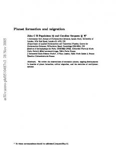
Rc [109 cm] Fig. 1. Comparison between the protoplanet effective radius for planetesimal capture. In solid line, R∗eff is calculated using Eq. (11) and in dashed–dotted line Reff is calculated including the gas drag of the atmosphere. These results were obtained with a full evolutionary numerical simulation. The protoplanetary disc surface density corresponds to a 6 MMSN. The protoplanet is located at 5.2 AU and the radius of incoming planetesimals is 100 km. (Press et al. 1992). The initial impact parameter considered for the integration of the trajectory is the effective radius in the absence of gas (Eq. (11), hereafter R∗eff ). Note that this is the lowest possible effective radius of the protoplanet. We calculated the trajectory of the planetesimal until it completes one close orbit inside the Hill sphere of the protoplanet (so it is always gravitationally dominated by the protoplanet). At this point, the planetesimal is considered captured and will definitely be accreted after a certain time. This procedure is repeated for increasing impact parameters (the relative difference between two consecutive trial impact parameters being 5 × 10−4 ) until the resulting orbit is no longer inside the Hill sphere. In other words, planetesimals are considered to be captured when the energy lost by gas drag allows them to complete one close orbit around the core and this is completely inside the protoplanet. The largest impact parameter for which this condition is fulfilled is adopted as the effective radius for that model. The solids accretion rate is still Eq. (10), using this new definition for Reff . The mass of accreted planetesimals is added to the mass of the core. It is worth mentioning that according to Inaba & Ikoma (2003), a detailed calculation of planetesimal ablation does not have a significant influence on the estimation of Reff . Note that our criterion for the capture of planetesimals and the determination of Reff is different to that employed by Pollack et al. (1996) where Reff is taken as the periapsis altitude of the outermost bound orbit. We performed a full evolutionary calculation of the formation of a giant planet in circular orbit around the Sun, with a = 5.2 AU, and immersed in a disc for which solids and gas densities are increased by a factor of 6 with respect to the MMSN (see Sect. 3.2). The effect of gas drag on the protoplanet effective radius is very important, as seen in Fig. 1. The effective radius calculated including the gas drag separates from the effective radius calculated according to Eq. (11), R∗eff , when the elapsed time is t ∼ 4 My and the radius of the core is Rc ∼ 109 cm. This corresponds to an envelope mass of ∼ 5 × 10−4 M⊕ and a core mass of ∼ 2 M⊕ . Note that by the end of the formation process, Reff is

5

more than 10 times larger than R∗eff . Moreover, it enters quadratically in the core accretion rate (Eq. (10)), so it will impact on the protoplanet formation timescale and on the final core mass (see Sect. 3). The core growth rate (Eq. (10)) depends also on the surface mass density of planetesimals, Σ, a quantity that is neither constant in time nor in space. Σ is a function of the distance to the central star (see Sect. 2.1) and also depends on the disc evolution. In this paper we consider only one effect for the time dependence of Σ: the accretion by the protoplanet. There are other important effects to be taken into account for a more realistic calculation of the planetesimal accretion rate, for example, planetesimal migration in the protoplanetary disc due to the nebular gas drag (Thommes et al. 2003) and planetary perturbations, for example, planetesimal ejection away from the feeding zone of the protoplanet (Alibert et al. 2005). However, this paper is mainly focused on the coupling of an oligarchic growth regime for the core with a full evolutionary calculation of the formation of a giant planet, so in this first exploration we shall neglect other effects that may contribute to the time evolution of Σ. When considering the time variation of Σ we assume that the growing protoplanet is able to capture planetesimals only from its feeding zone, defined as an annulus of 4 Hill radii (Eq. (9)) at either side of its orbit. The surface density inside the feeding zone at a certain time t is considered to be uniform, changing only due to the accretion by the protoplanet Σ ≡ hΣi (t) = hΣi0 −

Mc (t) , 2 π(aout (t) − a2int (t))

(16)

where aint (t), aout (t) are the inner and outer boundaries of the feeding zone and hΣi0 is the average of the initial surface density in that region. Adopting this expression for Σ tacitly implies that the accretion process is slow enough to guarantee a uniform distribution of planetesimals inside the feeding zone. 2.3. Interaction between incoming planetesimals and the protoplanetary envelope

On their trajectory to the core, accreted planetesimals interact with the gaseous envelope of the protoplanet exchanging energy. In this study, we implemented a simple model to take into account this effect (for more detailed models see Podolak et al. 1988; Pollack et al. 1996; Alibert et al. 2005). To simplify the situation, we assume planetesimals approaching the protoplanet as coming from infinity and entering the envelope with velocity vrel (Eq. (12)), describing afterwards a straight trajectory to the core. This may seem to contradict the fact that we calculate the orbits of planetesimals to define Reff , but as mentioned earlier we stop orbit calculation when planetesimals complete the first revolution inside the Hill sphere. In the future we will incorporate a complete calculation of the trajectories to the core, together with a self–consistent deposition of planetesimal energy in the gaseous layers of the envelope. In our simple model of a straight trajectory to the core, the energy of one incoming planetesimal of mass m at the top of the atmosphere is E=

1 2 mv . 2 rel

(17)

Gas drag and gravity acceleration are considered here as the two main responsible forces for changing the energy of planetesimals throughout the envelope. The drag force acting on a spherical planetesimal of radius rm and moving with velocity v is given

6


dv f = f D + f G = −m rˆ dt

(18)

and dv dv =v , dt dr

Mass [M⊕]

by Eq. (15). The gravitational force is calculated as usual with Eq. (14). Both forces act simultaneously and modify the planetesimal velocity. The total force acting on a planetesimal is

(19)

then

M Menv Mc

0

CD π rm2 ρg v GMr dv =− + 2 . dr 2m r v

dEk,m 1 dE =− = CD πrm2 ρg v2 . dr dr 2

(21)

These equations correspond to the energy exchange of one planetesimal with the surrounding gas. When considering all incoming planetesimals per unit of time, M˙ c , and transforming the differential equations into difference equations, the total variation of energy ∆Ei of the envelope’s shell i in the time interval ∆t is 1 M˙ c 2 ∆Ei = CD π rm2 ρg v ∆ri ∆t. 2 m i

(22)

(23)

2.4. The gaseous envelope

The general procedure employed in this study to numerically solve the formation of a giant planet was introduced in a previous paper (Benvenuto & Brunini 2005). In the above sections we mentioned some of the main improvements introduced to the model presented in that work. For the sake of completeness, we summarise here the fundamental ideas concerning the solution of the envelope’s structure. The full differential equations of giant planet formation are solved with an adaptation of a Henyey–type code. Radiative and convective transport are considered, employing the Schwarzshild criterion for the onset of convection. The adiabatic gradient is adopted for the temperature gradient in the latter case. The boundary conditions remain the same. As inner boundary conditions, we consider the core density to be constant, ρc = 3 g cm−3 . The mass of the core at time t is calculated as (24)

The luminosity on the surface of the core is Lr (Mc ) = 0,

15

20

25

Time [10 years] Fig. 2. Comparison case. We plot the mass evolution of the core (solid line), of the envelope (dash–dotted line) and of the total mass (dashed line) of the protoplanet. The input parameters of this run are the same as those of case J3 of Pollack et al. (1996). This figure should be compared to Fig. 2b of the cited article. See the text for details. and the velocity is v (Mc ) =

˙c M . 4 π R2c ρc

(26)

For the outer boundary conditions, the planetary radius is defined as (27)

where the accretion radius, Racc , is given by GM , (28) c2 c being the sound velocity. RH is the Hill radius (Eq. (9)). The external boundary conditions for the temperature and density of the envelope are those corresponding to the nebular gas, T and ρ (see Sect. 2.1). For further details on this aspect, we refer the reader to Benvenuto & Brunini (2005). Regarding the equation of state (EOS), we employ results presented in Saumon et al. (1995). For the grain opacities, we use the tables from Pollack et al. (1985). For temperatures above 103 K we consider Alexander & Ferguson (1994) molecular opacities which are available up to T ≤ 104 K and for higher temperatures we consider opacities by Rogers & Iglesias (1992). Racc =

Finally, when planetesimals reach the core, all their remaining kinetic energy is deposited in the adjacent gas shell.

4 π ρc R3c (t). 3

10

R = min[Racc , RH ],

where vi (the velocity of planetesimals when entering an envelope’s shell i) is obtained from a discretisation of Eq. (20),    CD π rm2 ρg vi−1 GMri−1/2   ∆ri−1 . + 2 vi = vi−1 + − 2m ri−1/2 vi−1 

5

6

(20)

The kinetic energy lost by a planetesimal due to gas drag Ek,m is transformed into heat, gained by the envelope’s shells,

Mc =

90 80 70 60 50 40 30 20 10 0

(25)

3. Results 3.1. Comparison with previous studies

To our knowledge, no self–consistent calculation of giant planet formation with a core growing according to the oligarchic model has been performed to date. To show the impact of the core accretion rate on the whole formation of a planet we performed a simulation to be compared with previous results obtained by authors adopting another core accretion model. For comparison we selected one of the simulations performed by Pollack et al. (1996), their case J3 for the formation of a Jupiter–like object. These authors adopted for the growth of the core the model of Lissauer (1987), which assumes a more rapid growth regime than the model of Ida & Makino (1993) adopted here. For this run, the protoplanetary disc at 5.2 AU and the accreted planetesimals are characterised as follows:


7

80

log(dM/dt) [M⊕/yr]

−4

i / i*

70

dMc/dt

60

−6

50

−8

40 30

dMenv/dt

−10

20

−12

10

e / e* ~ 4

0

−14 0

5

10

15

20

0

25

0.1

Time [106 years] Fig. 3. For the same comparison case as in Fig. 2, solid (dashed– dotted) line shows the time evolution of the logarithm of the core (envelope) growth rate.

– – – – –

initial solids surface density Σ = 15 g cm−2 , nebula volume density ρ = 5 × 10−11 g cm−3 , nebula temperature T = 150 K, planetesimal bulk density ρm = 1.39 g cm−3 , planetesimal radius rm = 100 km.

The initial mass of the core, Mc , is 0.1 M⊕ and the core density, ρc , is 3.2 g cm−3 . The resulting core and envelope mass evolution of our run is depicted in Fig. 2, which should be compared with Fig. 2b of Pollack et al. (1996). We use the same mass range in the Y axis to favour the comparison, although the run was completed successfully to the end, that is, until the total mass of the planet, M, is that of Jupiter (318 M⊕ ). From Fig. 2 it can be seen that in our calculation it takes 19 My for the mass of the envelope to equal the mass of the core, while in Pollack et al. (1996) the cross– over point (Mc = Menv ) is reached in only 1.51 My. As is immediately obvious, the time difference between both calculations is of approximately one order of magnitude. This is a significant difference if we keep in mind that the estimated lifetime of the solar nebula is less than 10 My. However, it is worth pointing out that the cross–over mass in both simulations is almost the same (∼ 29 M⊕ ). For the sake of completeness, we mention that the whole formation time is 20.6 My and the final mass of the core is 42 M⊕ . From the comparison of both figures, it can also be seen that we do not find three phases in the formation of the planet as Pollack et al. (1996) found in their simulations. The slow growth of the core guarantees a smooth variation of the slope of the Mc curve. No different growth regimes in the mass of the core or in the mass of the envelope can be distinguished before the runaway growth of the envelope. Moreover, in Fig. 3 we show in a logarithmic scale, the solids and the gas accretion rate. Pollack et al. (1996) obtained a different behaviour of the accretion rates which allowed them to define a short phase 1 in the growth of the protoplanet which ends when dMc /dt = dMenv /dt, and a longer phase 2 which ends when Mc = Menv . Phase 2 is characterised by a constant proportionality between dMc /dt and dMenv /dt. Phase 3 corresponds to the usual runaway growth of the envelope. From Fig. 3 we can see that a distinction between phase 1 and a phase 2 cannot be inferred from our simulation. The time derivative of the mass of the envelope is a monotonously increasing function, with no flat slope after it becomes larger than the core growth rate.

0.2 RH [AU]

0.3

0.4

Fig. 4. The impact of the selected model for the growth of the core. The solid line shows the ratio of eccentricities e/e∗ , where e is calculated according to Eq. (13) and e∗ according to the model adopted by Pollack et al. (1996). The dashed–dotted line plots the ratio of inclinations i/i∗ . While in our model i depends on e (i = e/2), in Pollack et al.(1996) i∗ remains constant during the entire simulation. For the X axis we selected the Hill radius in order to get rid of the different formation timescales of both simulations.

Our physical model is in essence the same as that of Pollack et al. (1996), except for the selection of the core accretion model and the treatment of the interaction between incoming planetesimals and the gaseous envelope of the protoplanet. Regarding the latter, as explained in Sect. 2.3, we consider a simple model for the energy deposition, while Pollack et al. (1996) developed a more complex model where the complete trajectories to the core of accreted planetesimals are calculated and planetesimal ablation is also taken into account. However, this can not be the main cause of such an important difference between the two formation timescales. Although this effect may be important in determining the internal structure of the protoplanet and may also modify the formation timescale, for this to happen a significant amount of gas bound to the core is needed. In the present simulation, it takes 10 My to form a core of 10 M⊕ , and the mass of the envelope at that stage is only 0.1 M⊕ . Hence, the main cause of the significant discrepancies between the timescales, must be the growth model for the core. We adopt an oligarchic growth for the core (with an enhanced effective radius due to the gas drag of the envelope), while Pollack et al. (1996) prescribed the more rapid accretion model of Lissauer (1987), also modified by the enhancement caused by the gas drag. According to their Eq. (1), the core accretion rate can be written as: dM = πR2 ΣΩFg dt

(29)

where R is the effective radius, Ω is the Keplerian angular velocity and Fg is the gravitational enhancement factor. Fg depends on the RMS values of the reduced eccentricities and inclinations, and on the reduced effective radius, eh,m ≡

a e RH

ih,m ≡

a i RH

dc ≡

R . RH

They calculate the numerical values of Fg using the formulae obtained by Greenzweig & Lissauer (1992). Their model assumes

8


that planetesimals’ inclinations depend only on planetesimalplanetesimal interactions and adopt for ih,m the formula: ih,m = √

ve,m 3ΩRH

(30)

where ve,m is the escape velocity from the surface of a planetesimal. Clearly, the inclination i∗ = ih,m RH /a remains constant during the entire calculation while ih,m decreases with time. On the other hand, they assume that eccentricities are controlled by both planetesimals and protoplanet stirring, and prescribe for the reduced eccentricity the equation eh,m = max(2ih,m , 2).

(31)

This means that if eh,m = 2ih,m the protoplanet is growing according to the runaway regime, as e and i would be independent of the mass of the protoplanet, while if eh,m = 2 the eccentricity of planetesimals would be affected by the presence of the protoplanet, this condition corresponding to the protoplanet– planetesimal scattering in the shear–dominated regime. The numerical simulations of Ida & Makino (1993) showed that the protoplanet-planetesimal scattering in the shear–dominated regime lasts for only a few thousand years, after which planetesimals are strongly perturbed by the protoplanet, and the post–runaway regime can then be considered as a dispersion– dominated regime. In the dispersion–dominated regime eccentricities and inclinations satisfy that eh,m /ih,m ≃ 2 and eh,m > 2. Hence, in a model where the protoplanet–planetesimal scattering is in the shear–dominated regime, eccentricities and inclinations of planetesimals in the vicinity of the protoplanet remain low. This leads to an accretion scenario which is much faster than that corresponding to the oligarchic regime. To show the difference between eccentricities and inclinations in both models throughout the formation of the planet, we included in our simulation of the case J3, the calculation of ih,m and eh,m according to Eqs. (30) and (31). The ratio of the eccentricity and inclination between the two models is shown in Fig. 4. We chose the X axis to be the Hill radius of the protoplanet, as it is completely independent of time and the comparison is then straightforward. For this case, the initial value of ih,m is lower than 1 and, as it is a decreasing function of the mass of the protoplanet, eh,m always equals 2. Consequently, our eccentricities are larger than those in Pollack et al. (1996) by a factor of 4, as can be seen from Fig. 4. On the other hand, our inclinations are much higher (their inclination is constant throughout the whole formation of the planet, i∗ ≃ 0.0039), which impacts not only in the relative velocities but also in the scale height of the planetesimal disc which is inversely proportional to the core accretion rate. As a consequence, due to our larger eccentricities and inclinations, we obtain a much lower accretion rate and a longer formation timescale. Pollack et al. (1996) adopt for the definition of the boundaries of the feeding zone that the q radial distance on either side of the orbit is given by ∆a = 12 + e2h,m RH . According to our simulation, eh,m is always equal to 2, which leads to ∆a = 4RH , the same value we adopted in our calculations. 3.2. Results of full calculations of giant planet formation with an oligarchic growth for the core

All the simulations presented in this section were started with an embryo of 0.005 M⊕ , revolving in a circular orbit around the Sun. The semi–major axis of the orbit is that corresponding to

Jupiter, 5.2 AU. The mass of the seed was chosen to guarantee that the embryo is undergoing an oligarchic growth and that it is also able to bind a tiny atmosphere, the latter in order to allow the code to converge. The density of the core will be held constant during the entire formation process, ρcore = 3 g cm−3 . The discrepancy between core density and planetesimals bulk density (ρm = 1.5 g cm−3 ) is due to the progressive high pressure the core is subject to. We arbitrarily stopped calculations when the total mass of the protoplanet was that of Jupiter. This assumption tacitly implies that the nebula can always provide the necessary amount of gas for the formation of the planet. The first set of simulations is intended to show the consequences of the envelope’s drag on the oligarchic growth of the core (Eq. (10)). To this end, we performed several runs for various protoplanetary disc surface densities, including and excluding the effect of the gas drag in the calculation of Reff . The planetesimal radius is assumed to be constant, fixed for these examples at 100 km (no size distribution or collisions between planetesimals were taken into account). As no planetesimal migration, planetesimal ejection by the protoplanet, perturbations by other embryos, etc., were considered, the variation of the solid surface density of the feeding zone is only due to planet accretion. Since no mechanisms for the dissipation of the gaseous component of the nebula were modelled, the variation of the volume gas density of the feeding zone is due only to the formation of the envelope. We note that this is an idealised situation where the protoplanet probably has the largest amount of available material to feed itself. We found that, in spite of the favourable conditions for mass accretion of our model, for protoplanetary discs with densities lower than that of a 6 MMSN, the formation process could not be completed according to the timescales imposed by the observations of circumstellar discs (lower than 107 yr) in either of the cases considered for the calculation of Reff . The results for a disc of 6 MMSN are depicted in Fig. 5. The upper panel (Fig. 5 a) shows the evolution of the core and envelope mass when ignoring for the protoplanet capture effective radius the presence of the atmosphere (R∗eff calculated according to Eq. (11)). The complete formation of a Jupiter–mass object takes a bit over 17 My and the final mass of the core is ≃ 28 M⊕ (note that, in our model, all accreted solids are deposited onto the core). However, when including the atmospheric gas drag, the timescale turns out to be 12 My (still over the limiting 10 My) while the mass of the core increases to 60 M⊕ (see Fig. 5 b). This means that, in this case, the effect of the gas drag of the atmosphere reduces the formation time in about 30%, but also affects the final mass of the core, which is increased a factor of 2. Although a core of ∼ 10 M⊕ (currently an acceptable value for Jupiter’s core mass, Saumon & Guillot 2004) is formed in ∼ 6.5 My in the second simulation, the runaway collapse of the gaseous envelope occurs ∼ 5 My later. As seen from Eq. (10), the solids accretion rate is directly proportional to the solids surface density and the fact that the feeding zone is far from being depleted when this mass is achieved (see Fig. 6), allows the protoplanet continue the accretion of solids. In fact, as seen from Fig. 7, the peak of the core accretion rate takes place for t ∼ 8 My, when the mass of the core is approximately 20 M⊕ . This large number of incoming planetesimals contribute to the gas pressure supporting the envelope via their gravitational energy, and thus prevent faster accretion of gas from the nebula and as such permit the formation of a massive core. The same behaviour is found when increasing the surface density of the disc. In Table 2 we show, in round numbers, the formation times and the final masses of protoplanetary cores for


1.2e−05

a Mass [M⊕]

dMc/dt [M⊕/year]

Menv

100 40

Mc

30 20 10

1e−05 8e−06 6e−06 4e−06 2e−06

0 0

3

6

9

12

15

0

18

0

6

Time [10 years]

Mass [M⊕]

4

6

8

10

12

Fig. 7. This figure shows the evolution of the core accretion rate for the simulation that includes atmospheric gas drag. Note that the accretion rate is still an increasing function when the mass of the core reaches 10 M⊕ (corresponding to ∼ 6.5 My; see also Fig. 5 b), preventing the rapid accretion of the envelope mass.

100 Menv

80

2

Time [106 years]

b

60

Table 2. Comparison of formation times and core masses for several disc densities. Planetesimal radius is 100 km.

Mc

40 20

Disc density [MMSN]

Without gas drag Formation Core time [My] mass [M⊕ ]

With gas drag Formation Core time [My] mass [M⊕ ]

6 7 8 9 10

17 14 11 10 8

12 9 7 6 5

0 0

3

6

9

12

15

6

Time [10 years]

Fig. 5. For a 6 MMSN protoplanetary disc, panel a shows the core (solid line) and envelope (dashed–dotted line) mass evolution of a Jupiter–like forming protoplanet at 5.2 AU, considering that the core grows according to the oligarchic growth regime, with R∗eff calculated with Eq. (11). Panel b shows the same simulation but including the gas drag effect of the protoplanetary atmosphere in the calculation of Reff . Note that for a clear visualisation the Y axis changes from a linear scale to a logarithmic scale. Panel a (b) is in a linear scale up to 40 M⊕ (100 M⊕ ), afterwards the scale is logarithmic. For both runs, planetesimal radius was set equal to 100 km. Surface Solid Density [gr cm−2]

9

24 20 16 12 8 4 0 0

2

4

6

8

10

12

14

6

Time [10 years]

Fig. 6. This panel depicts the evolution of the solids surface density for the simulation that includes the atmospheric gas drag (corresponding to Fig. 5 b). A core of ∼ 10 M⊕ is achieved for t ∼ 6.5 My, when Σ is still very high.

28 32 36 40 43

60 70 81 91 100

Table 3. Comparison of formation times and core masses for several disc densities with a planetesimal radius of 10 km. Disc density [MMSN]

Without gas drag Formation Core time [My] mass [M⊕ ]

With gas drag Formation Core time [My] mass [M⊕ ]

6 7 8 9 10

9 7 6 4.8 4

5.6 4 3 2.2 1.75

34 40 45 50 55

69 80 92 104 115

discs that range from 6 MMSN to 10 MMSN and planetesimals having a radius of 100 km. As expected, the higher the density of the disc, the shorter the formation time but the larger the final core’s mass (see also Pollack et al. 1996). The timescale reduction, when the gas drag from the atmosphere is included, ranges from ∼ 30% for 6 MMSN to ∼ 40% for 10 MMSN. The maximum timescale reduction for these cases is then less than a factor of 2. The mass of the core, on the other hand, monotonously increases fractionally, from a factor of ∼ 2.15 for 6 MMSN to a factor of ∼ 2.35 for 10 MMSN. Qualitatively, all curves look similar to that shown in Fig. 5 and it is not worth showing them here. When the same comparative simulations are made for planetesimals having a radius of 10 km (this means, simulations that consider both cases for the effective radius of the protoplanet,

10


a

100 Mass [M⊕]

Menv

40

Mc

30 20 10 0 0

1

2

3

4

5

6

7

8

9

10

6

Time [10 years]

b Mass [M⊕]

100

Menv

80 60 Mc

40 20 0 0

1

2

3

4

5

6

6

Time [10 years]

Fig. 8. For a protoplanetary disc of 6 MMSN and planetesimals having a radius of 10 km, upper panel (a) shows the evolution of the protoplanet mass (the core mass with the solid line, the envelope mass with the dashed–dotted line) when no atmospheric gas drag is considered. The lower panel (b) illustrates the same process but when Reff is calculated including the gas drag force acting on incoming planetesimals. Again, the Y axis is split in two different scales: first we adopt a linear scale and then a logarithmic one. The same range as in Fig. (5) is adopted.

R∗eff and Reff ), the timescale reduction ranges from ∼ 38% for 6 MMSN to ∼ 56% for 10 MMSN, and again we find that the mass of the core is doubled (see Table 3). For planetesimals of this size, and according to the results presented in Table 3, one could speculate about reducing the density of the disc (to less than that corresponding to 6 MMSN) and still finding a formation timescale below 107 yr (when considering the enhanced capture radius by gas drag). However, to present our results clearly, we find it more relevant to compare the several sets of simulations for the same nebula conditions. For the sake of completeness, Fig. 8 shows the evolution of the core mass and the envelope mass for a 6 MMSN disc where the planetesimal radius is 10 km. When gas drag from the envelope of the protoplanet is ignored, the formation time is ∼ 9 My and the core mass is ∼ 34 M⊕ . However, when this effect is included in the calculations, the total formation time is reduced to ∼ 6 My, with a final super–massive core of 69 M⊕ . Although our core masses are in all cases completely out of range for present models of Jupiter total mass of solids, MZ (recent estimations are Mc < ∼ 11 M⊕ and 1 M⊕ < ∼ Mc + MZ < ∼ 39 M⊕ , Saumon & Guillot 2004), the main objective of this work is not directed to fit our results to these values, but on stressing

the results obtained when adopting the oligarchic growth for the core. From our calculations it is clear that including the enhancement of the accretion cross–section due to gas drag, helps to reduce the formation timescale when considering an oligarchic model, although surface densities higher than that of the MMSN are still needed. The main drawback of these massive discs is that they lead to the formation of super–massive cores. However, we have to keep in mind that no mechanisms of planetesimal removal from the feeding zone of the protoplanet are taken into account, except for the depletion due to planetesimal accretion onto the protoplanet. Thommes et al. (2003) calculated analytically and numerically the evolution of solid protoplanetary masses growing oligarchical for a wide range of semi–major axes and for a protoplanetary disc of 1 MMSN and 10 MMSN (their solids surface density for the MMSN is slightly lower than ours). For a 10 MMSN and considering planetesimals having a radius of 10 km, they obtain a protoplanet of ≃ 60 M⊕ , a result we were also able to reproduce in the absence of gas accretion. However, when they include in their simulations the planetesimal migration in the protoplanetary disc due to nebular gas drag, the resulting protoplanet is reduced to ∼ 10 M⊕ . Planetesimal migration due to gas drag is a relevant ingredient which should be considered in future calculations for an accurate estimation of the mass of the core and of the formation timescale. Another important effect that should be taken into account in future calculations is the ejection of planetesimals out of the feeding zone. This could probably also help in solving the problem of having a Jupiter– like planet with such large core masses. Since ejection occurs mainly for large mass planets, this would not necessarily slow down the accretion of planetesimals at the beginning, and may not lead to a too long formation time of the planet. The previous paragraphs focus on the consequences of the enhancement of the effective capture cross–section due to the envelope’s gas drag. We now analyse the importance of planetesimal size. For a clear visualisation we summarise in Table 4 the earlier calculations with the enhanced effective radius for planetesimals having radii of 10 and 100 km. Planetesimal mass appears in Eq. (13), which determines the relative velocity of planetesimals with respect to the protoplanet through Eq. (12). Smaller planetesimals experience stronger damping of random velocities due to nebular gas and form a thinner disc (i ≃ 12 e and h ≃ a i) which in turn favours accretion (Thommes et al. 2003). Moreover, smaller planetesimals suffer from a stronger deceleration due to atmospheric gas drag, increasing the impact parameter. Both effects combined favour the formation process, reducing the formation timescale. If we analyse and compare results without including the gas drag of the envelope for a fixed nebula density (first and second Cols. of Tables 2 and 3), we find that for planetesimal radius of 10 km the whole formation process is reduced in an approximately constant factor of 2 when compared to planetesimals having a radius of 100 km, while the core mass is increased by 25%. This value is independent of the protoplanetary disc conditions, at least in the cases considered here. When the gas drag is included in the calculations this behaviour changes (see Table 4). Results show that the formation time reduces from a factor of ∼ 2 for a protoplanetary disc of 6 MMSN to a factor of ∼ 3 in the case of 10 MMSN, when comparing the runs for the same protoplanetary disc conditions but for different planetesimal size. The factor of the timescale reduction depends then, on the surface density of the protoplanetary disc. The mass of the core is less affected than in the previous case, resulting for planetesimals having a radius of 10 km, as being on average, 15% more


Table 4. Comparison of formation times and core masses for several disc densities, and for two different planetesimal sizes: 100 and 10 km. All cases were calculated including atmospheric gas drag. Disc Planetesimal density radius: 100 km [MMSN] Formation Core mass time [M⊕ ] [My]

Planetesimal radius: 10 km Formation Core mass time [M⊕ ] [My]

6 7 8 9 10

5.6 4 3 2.2 1.75

12 9 7 6 5

60 70 81 91 100

69 80 92 104 115

massive than for planetesimal radius of 100 km. These results show that when including the gas drag of the envelope, the reduction factor in the formation time also depends on the surface density of the disc. Note that the fractional decrease of the whole formation time is greater than the fractional increase of the core mass. In summary, this section focused on the study of the formation of a giant planet with a full evolutionary code, assuming an oligarchic growth regime for the core. We first studied the enhancement of the effective capture radius due to the presence of the gaseous envelope. The atmospheric gas drag enlarges the capture cross–section, causing a reduction in the formation time but also a significant increment in the mass of the core. We also studied the impact of the size of accreted planetesimals in our model. We found that the whole formation process is accelerated when considering smaller planetesimals and that the reduction factor depends on the surface density of the feeding zone. However, no substantial change in the final mass of the core was identified.

4. Discussion and summary In this paper we examined the formation of a Jupiter–like object. Motivated by the work of Thommes et al. (2003), we selected an oligarchic growth regime for the core as the planetesimal accretion rate. The numerical simulations were made with the code presented in a previous paper by Benvenuto & Brunini (2005), which was updated in this study (see Sect. 2). This code was developed for a self–consistent calculation of giant planet formation, so the growth of the core is coupled to the growth of the envelope. In this sense, the evolution of the envelope’s density profile is a natural outcome of the code and a relevant quantity for an accurate estimation of the enhancement in the protoplanet capture cross–section of planetesimals (as the drag force depends on ρg , see Eq. (15)), which has a direct impact on the growth rate of the core. When including a time–dependent planetesimal accretion rate in these kinds of calculations, most authors prescribe a rapid one, that in general guarantees the formation of a massive core in a few hundred thousand years. However, N–body simulations show that when the embryo is about the mass of the Moon, or even smaller (Thommes et al. 2003), the growth regime enters the protoplanet–dominated stage. For this reason, we assume from the very beginning of our calculations an oligarchic growth regime, which seems to be a more realistic approach to the problem. This accretion rate is considerably slower than the usually–adopted accretion model of Greenzweig & Lissauer

11

(1992). Adopting the oligarchic growth model has, as a main consequence, an increase in the whole formation timescale when compared to previous calculations which adopt a rapid growth for the core (see Sect. 3.1). In this sense, it is worth mentioning that an accurate giant planet formation model with an oligarchic growth for the core should also include planetesimal migration due to the nebular gas drag since the assumed lifetime of the nebula is of the same order of magnitude of the formation process itself (Thommes et al. 2003). In the calculations presented here this effect was not included, as this article aims to analyse in a first approximation the oligarchic growth regime for a giant planet in a self–consistent calculation. To the authors’ knowledge, the oligarchic growth of protoplanets has generally been studied in the absence of an atmosphere and no full evolutionary calculations of gaseous giant planets adopting this growth regime for the core have been performed in the past. As giant planets have large gaseous envelopes, the gas drag effect of the growing atmosphere should play an important role in the resulting accretion cross–section of the protoplanet. In order to study the relevance of this effect, we made a set of simulations for several disc densities to estimate the consequences of including the gas drag in the calculation of the effective radius and we compared them to those where the effective radius is calculated in the absence of gas drag. According to our simulations, the main effects of the enlargement of the effective radius when considering the gas drag are a reduction of about 30% to 55% in the whole formation timescale (depending on the surface density of the disc and on the planetesimal mass, being stronger for smaller planetesimals) and an increase in the mass of the core by about a factor of 2 for the several protoplanetary disc considered here. As we mentioned before, no planetesimal migration or other protoplanet–disc interactions were considered, so our results should be analysed in the context of this simple model. However, from the comparison of simulations with and without atmospheric gas drag, we conclude that including the gas drag in the calculation of the effective cross–section of the protoplanet is absolutely relevant to the estimation of the formation timescale. The fact that, in association with higher surface densities for the disc, we obtain the desired shorter timescales but, on the other hand, super–massive cores should not be a cause for concern. Although the mass of the core is closely related to the formation timescale (the more massive the core, the shorter the timescale), Thommes et al. (2003) showed in their calculations of the formation of protoplanetary cores, that planetesimal migration strongly affects the planetesimal population of the feeding zone, being very effective in depleting it. Including this effect reduces considerably the final mass of the core, and protoplanetary discs as massive as 10 MMSN would probably offer us good fits to the core mass and the formation timescale simultaneously. In this paper, we also explored the effect on giant planet formation of planetesimal size variations. For the same set of protoplanetary discs (from 6 to 10 MMSN), we made simulations for a swarm of planetesimals having a fixed radius of 10 and 100 km. We find that the formation timescale is strongly dependent on planetesimal size: for planetesimal radius of 10 km, the process occurs a factor of 2 to 3 times faster than for the case of larger planetesimals. A reduction in the timescale was expected, since smaller planetesimals have lower relative velocities which favour accretion and they are much more affected by gas drag. However, the mass of the core is not very increased. In a recent paper, Inaba & Ikoma (2003) also explored the effects of gas drag on the effective radius of a protoplanet for capturing planetesimals of different sizes. They found that gas

12


drag largely increases the effective capture radius. While our results are qualitatively similar to those of Inaba & Ikoma (2003), we note that we employed a full evolutionary code. In particular, it is worth discussing the results Inaba & Ikoma (2003) presented in their Fig. 6. They estimated the time spent in forming a 10 M⊕ core as a function of planetesimal size, finding that gas drag drastically decreases the formation timescale: for planetesimals of, e.g., 10 km (100 km) the timescale is reduced by a factor of ∼ 6 (∼ 4). These factors would be very helpful in alleviating the timescale problem of the whole core growth mechanism. However, the results presented in this paper indicate that, while there exists a reduction in the time spent in forming a core of 10 M⊕ , it is much more modest. We find that it is only slightly dependent on the protoplanetary surface density and moderately dependent on the planetesimal size. For planetesimals of 10 km the average reduction factor in the formation timescale of a 10 M⊕ core is ∼ 1.25 and for planetesimals of 100 km it is ∼ 1.5. It is also worth mentioning that the timescale involved in forming a 10 M⊕ core is not really representative of the complete giant planet formation timescale as shown in this and previous papers (e.g., Pollack et al. 1996). The next step for our future calculations is the inclusion of planetesimal migration due to nebular gas drag and planetesimal ejection out of the feeding zone. This will provide us with a more accurate quantitative idea of the final core masses and formation timescales in the frame of an oligarchic growth regime for the core. Also, a size distribution of the accreted planetesimals should be considered for a better estimation of the formation timescales. Or, at least, if a unique radius is adopted for all planetesimals in the swarm, several simulations varying the radius should be made in order to bracket the formation time. Finally, we expect to update the opacity tables since opacity plays a fundamental role in the formation timescale (Podolak 2003; Hubickyj et al. 2005). It would also be interesting to test with our model, the response of the whole planetary formation process to grain opacity reduction, which will probably shorten the timescales involved, as has been already shown by, e.g., Pollack et al. (1996) and Hubickyj et al. (2005). Acknowledgements. A.B. acknowledges the financial support by ANPCyT. The authors wish to thank the anonymous referee for constructive criticisms which enabled us to largely improve the original version of this article.

References Adachi, I., Hayashi, C., & Nakazawa, K. 1976, Progress of Theoretical Physics, 56, 1756 Alexander, D. R., & Ferguson, J. W. 1994, ApJ, 437, 879 Alibert, Y., Mordasini, C., Benz, W., & Winisdoerffer, C. 2005, A&A, 434, 343 Benvenuto, O. G., & Brunini, A. 2005, MNRAS, 356, 1383 Bodenheimer, P., & Pollack, J. B. 1986, Icarus, 67, 391 Chambers, J. 2006, Icarus, 180, 496 Chen, C. H., & Kamp, I. 2004, ApJ, 602, 985 Durisen, R. H., Boss, A. P., Mayer, L. et al. 2007, in Protostars and Planets V. Edited by B. Reipurth, D. Jewitt, & K. Keil. (University of Arisona Press, Tucson), 591 Greenberg, R., Hartmann, W. K., Chapman, C. R., & Wacker, J. F. 1978, Icarus, 35, 1 Greenzweig, Y., & Lissauer, J. J. 1992, Icarus, 100, 440 Haisch, K. E., Jr., Lada, E. A., & Lada, C. J. 2001, ApJ, 553, L153 Hayashi, C. 1981, Progress of Theoretical Physics Supplement, 70, 35 Hubickyj, O., Bodenheimer, P., & Lissauer, J. J. 2005, Icarus, 179, 415 Ida, S., & Makino, J. 1993, Icarus, 106, 210 Inaba, S., & Ikoma, M. 2003, A&A, 410, 711 Klahr, H., & Bodenheimer, P. 2006, ApJ, 639, 432 Kokubo, E., & Ida, S. 1996, Icarus, 123, 180 Kokubo, E., & Ida, S. 1998, Icarus, 131, 171 Kokubo, E., & Ida, S. 2000, Icarus, 143, 15 Kokubo, E., & Ida, S. 2002, ApJ, 581, 666

Lissauer, J. J. 1987, Icarus, 69, 249 Lissauer, J. J., & Stevenson, D. J. 2007, in Protostars and Planets V. Edited by B. Reipurth, D. Jewitt, & K. Keil. (University of Arisona Press, Tucson), 607 Mayor, M., & Queloz, D. 1995, Nature, 378, 355 Mizuno, H. 1980, Progress of Theoretical Physics, 64, 544 Press, W. H., Flannery, B. P., Teukolsky, S. A., & Vetterling, W. T. 1992, Numerical Recipes: The Art of Scientific Computing, Third Edition, Cambridge University Pess , Cambridge Podolak, M., Pollack, J. B., & Reynolds, R. T. 1988, Icarus, 73, 163 Podolak, M. 2003, Icarus, 165, 428 Pollack, J. B., McKay, C. P., & Christofferson, B. M. 1985, Icarus, 64, 471 Pollack, J. B., Hubickyj, O., Bodenheimer, P. et al. 1996, Icarus, 124, 62 Rogers, F. J., & Iglesias, C. A. 1992, ApJ, 401, 361 Safranov, V.S. 1969, in Evolution of of the Protoplanetary Cloud and Formation of the Earth and Planets. Nauka, Moscow [Engl. tansl. NASA TTF-677, 1972] Saumon, D., Chabrier, G., & van Horn, H. M. 1995, ApJS, 99, 713 Saumon, D., & Guillot, T. 2004, ApJ, 609, 1170 Thommes, E. W., Duncan, M. J., & Levison, H. F. 2003, Icarus, 161, 431 Wuchterl, G., Guillot, T., & Lissauer, J. J. 2000, Protostars and Planets IV, 1081