in: Proc. IEEE/RSJ Int. Conf. on Intell. Robots and Systems (IROS 2003), Las Vegas, pp. 1505-1511, IEEE omnipress 2003
Omnivision-based Probabilistic Self-localization for a Mobile Shopping Assistant Continued Horst-Michael Gross, Alexander Koenig, Christof Schroeter and Hans-Joachim Boehme Ilmenau Technical University, Department of Neuroinformatics 98684 Ilmenau, GERMANY
[email protected]
I. I NTRODUCTION AND MOTIVATION In [3] we introduced our long-term research project PERSES (PERsonal SErvice System) which aims to develop an interactive mobile shopping assistant which can autonomously guide its user, a customer, to desired articles within a home store realizing a guidance function, or follow him as a mobile service-companion while continuously observing the user and his behavior. To accommodate the challenges that arise from the specifics of this interaction-oriented scenario and the characteristics of the operation area, a very regularly structured, maze-like environment, we placed special emphasis on vision-based methods for both human-robot interaction and robot navigation. Because the topology of such a home store shows many similar, long hallways of equal length, width and geometrical structure, self-localization methods based on laser or sonar produce numerous ambiguities complicating a quick self-localization or re-localization in case of a complete loss of positioning. Moreover, 2Ddistance sensors only operate at certain planes of the 3D space. Therefore, empty goods shelves show blank space at the respective height which can be misinterpreted as free space. Vision-based systems, however, do not show these limitations, but supply a much greater wealth of
panoramic image
sector-based feature extraction
Monte Carlo Localization last robot movement ut-1 = (dx, dy, dϕ)
omnidirectional color view
Abstract— In continuation of [3], where we presented the basic idea of our omniview-based MCL approach (Fig. 1) and preliminary experimental results, this paper describes a number of methodical and technical improvements addressing challenges arising from the characteristics of our realworld application, the vision-based self-localization of a mobile robot acting as shopping assistant in a maze-like environment, a home store. To cope with highly varying illumination conditions, we present a reference-based correction approach that realizes a robust, automatic luminance stabilization and color adaptation already at the level of image formation. To deal with severe occlusions or disturbances of the omnidirectional image caused by, e.g. people standing nearby the robot or local illumination artifacts, we introduce a novel selective observation comparison method as prerequisite for a robust particle filter update. Further studies investigate the impact of the utilized observation model on the localization accuracy. The results of a series of localization experiments carried out in the home store (see video) confirm the robustness and superiority of our advanced, real-time approach and outperform the localization results obtained so far.
• Prediction phase • Update phase & resampling (i)
{ô t } i =1...N
learned graph representation of the operation area
ϕ y
sample set x
sampling-based multi-modal density representation
Bel( x t ) = { x t , wt(i) } i =1...N (i)
nodes labeled with reference observations or and metric data about the robot‘s pose xt
Fig. 1. General idea of our omniview-based MCL. The approach is based on a graph-based representation of the operation area. The nodes of the graph are labeled with view-based reference observations and metric information about the robot’s pose at the moment of node insertion.
information about the 3D-structure of the hallways. For example, the filling of the goods shelves with different articles gives the hallways a characteristic appearance, especially with respect to color or texture. Because of this, we expected to defuse the localization problem drastically by development of an approach for vision-based localization that combines omnivision with probabilistic self-localization techniques. In recent years, a number of omnivision-based robot localization approaches have been proposed. Most of them construct appearance models of the environment by compressing the captured panoramic snapshots of interesting locations using eigenspace representations, or apply specific image processing methods (e.g., image histogram matching [8]), to localize and track the robot. Several of the eigenspace approaches employ a subset of the principal components [4], [6], other ones use an illumination independent filtering of the eigenspace data [5], exploit an eigenspace approximation to distortion insensitive distance measures [9], or employ Bayesian reasoning over the features of panoramic eigenimages [7], to achieve a robust localization under illumination changes or image occlusions. However, in most of these approaches localization is typically performed in a straightforward way: the current input image or its sub-space projection
is compared to all reference images, and that location whose reference image best matches the current input is considered to be the location currently taken by the robot. Instead of using highly sophisticated image compression and feature selection techniques followed by a classifying mapping from the current observation to the best fitting internal representation, we favor the opposite way, namely a relatively simple pre-processing and feature extraction in combination with a distributed probabilistic multi-hypothesis estimation. This allows to generate and track a set of alternative location hypotheses in parallel which can be disambiguated in the following actionperception-cycles. The reason is, that in ambiguous, mazelike environments, localization on the basis of a crisp mapping from observation o to state x becomes very unreliable. Therefore, probabilistic methods, like Bayes filters, are required to quantify the ambiguity by means of beliefs for multiple location hypotheses. In [3] we introduced the basic idea and essential aspects of our omniview-based Monte Carlo Localization and presented first promising experimental results as work in progress. A short recapitulation of our approach will be given in the next section, before we present improved aspects and new experimental results in section III. II. S UMMARY OF OUR LOCALIZATION APPROACH Our omniview-based probabilistic self-localization approach presented in [3] is a version of the Monte Carlo Localization (MCL) [1], [2] and makes use of particle filters for approximating a multi-modal density distribution coding the robot’s belief Bel(xt ) for being in state xt = (x, y, ϕ )t in its state space. x and y are the robot’s position coordinates in a world-centered Cartesian reference frame, and ϕ is the robot’s heading direction. The key idea of MCL is to represent the belief Bel(xt ) for being in the current state xt by a set St of N weighted samples (i) (i) distributed according to Bel(xt ): St = {xt , wt }i=1..N . (i) (i) Here each xt is a sample, and the wt are non-negative importance weights. Because the sample set constitutes a discrete approximation of the continuous density distribution, particle filters are computationally efficient since they focus the particles on those regions in state space with high likelihood, where things really matter. The general idea of our omniview-based MCL is illustrated in Fig. 1. As map of the environment, our approach employs a graph representation of the environment (Fig. 1, bottom right) which is learned on-the-fly while manually joy-sticking the robot through the operation area. Each node of the graph is labeled with both visual reference observations or (x, y, ϕ ) extracted from the respective panoramic view at position x, y in heading direction ϕ and the corresponding odometric data about the correct pose at the moment of the node insertion during teaching. A new node (reference point) is inserted, either if the
Euclidian position distance to other reference points in a local vicinity or if the Euclidian feature distance between the current observation ot and the reference observations or (x, y, ϕ ) at adjacent reference points are larger than given threshold values. The labeling of the graph nodes with odometric data about the pose of the robot, however, necessitates an efficient correction of odometry because of the increasing error over time, especially concerning the orientation angle. To attenuate this effect, we utilize a specific feature of the market floor that shows a very regular structure caused by tiles which are uniquely oriented across the whole market. Details of our vision-based odometry correction are presented in [3]. We successfully utilize this odometry correction for learning of consistent, large-scale graph representations of the operation area. 1) Feature extraction for observations: Both during map-building and self-localization, the omnidirectional image is transformed into a panoramic image (Fig. 1, top) that is partitioned into a fixed number of non-overlapping sectors. The following criteria determined the selection of appropriate features to describe the omniview: a) To allow for an on-line localization, the calculation of the features should be as easy and efficient as possible. b) The feature set should include the orientation of the robot as prerequisite to estimate its heading direction. c) It should allow an easy generation of expected observations for hypothetical poses of the robot. Considering these criteria and the requirements of other omnivision-based localization approaches published recently, e.g. [9], [8], [6], [7], we decided to implement the simplest feature extraction method possible: for each segment of the panoramic image only the mean RGB-values are determined. 2) The localization algorithm: The prediction and correction update of the sample set is achieved by a procedure often referred to as Sequential Importance Sampling with Resampling. In the Prediction phase (robot motion), the sample set computed in the previous iteration (or during initialization) is moved according to the last movement of the robot ut−1 (Fig. 1, left). Here, the motion model p(xt |xt−1 , ut−1 ) defines how the position of the samples changes using information ut−1 from odometry. This way, MCL generates N new samples that approximate the expected density distribution of the robot’s pose after the movement ut−1 . To determine the expected observations (i) oˆ t of the moved samples i, our approach requires interpolations both in state and feature space because of the coarse graph representation and the chosen feature coding. Therefore, for each sample s(i) , we first interpolate linearly between the reference observations or (x) of the two reference nodes closest to the respective sample (i) position xt . After this, the resulting feature vector is (i) rotated according to the expected new orientation ϕt of (i) the sample s , utilizing a linear interpolation between the features of adjacent segments. This way, we obtain a set of
(i)
N new feature vectors oˆ t (x, y, ϕ ) describing the expected (i) observations of the moved samples in the new states xt . In the Update phase (new observation), the actual observation ot at the new robot position has to be taken into account in order to correct the sample set St . For this, the (i) importance weight wt of each sample s(i) is computed. It describes the probability that the robot is located in the (i) state xt of the sample. The weights are determined from (i) the errors Et between the current observation ot at the (i) new robot position and the expected observation oˆ t of each sample s(i) applying the camera-specific observation model p(ot |xt ) = f (Et ) which returns the likelihood of an observation error for a given pose (see Sec. III-D.1). This (i) (i) way, the weights wt = α · f (Et ) are determined, where ( j) α is a normalization constant that enforces ∑Nj=1 wt = 1. The final sample set St for the next iteration is obtained by resampling from this weighted set. The resampling selects those samples with higher probability that have high importance weights. Samples with low weights are removed and randomly placed in the state-neighborhood of samples with high weights. 3) Previous experiments and problems encountered: All experiments were carried out in a large home store with our experimental platform PERSES, a standard B21 robot additionally equipped with an omnidirectional imaging system for vision-based navigation and humanrobot interaction (Fig. 1, left). Our previous experiments reported on in [3] were performed as simple off-line cross-validation tests on different subsets of observation sequences captured while manually joy-sticking the robot through the store. A subset of these pose-labeled omniviews (about 2.000) was used as reference observations or (x, y, ϕ ) to build the graph while the other ones, the “unknown” omniviews (about 6.000) captured between the reference points along the traveled known route, were used as test data to determine the localization errors in a series of experiments. The achieved results confirmed the general efficiency and accuracy of our omniview-based probabilistic self-localization method. In the practical application of our approach, however, several problems occurred which forced us to further improve technical and methodical aspects of our omniviewbased MCL-system. Moreover, we introduced a new experimental regime which consequently distinguishes between training tours traveled to build the graph and test tours executed to acquire data (unknown observations labeled with the robot’s poses) for the localization experiments. Now, the period of time between training tour and test tours can be chosen between a couple of hours at the same day and a few days or weeks, in order to selectively investigate specific real-world effects, like illumination changes or appearance variations (see section III-D). To cope with highly varying illumination
conditions, we developed a very effective, reference-based color and luminance adaption mechanism (see section IIIA). Because occlusions of the omniview are not only a result of people standing nearby the robot or objects being moved around, but also of local illumination artifacts, we developed a more selective mechanism for the comparison between expected observations and actual observation as prerequisite for the particle filter update (sec. III-B). Other studies dealt with the impact of the used observation model and the influence of a new type of particles (grounded particles) on the accuracy of the pose estimation (sec. III-D.1, III-C). III. I MPROVEMENTS AND NEW RESULTS A. Luminance stabilization and color adaptation Highly varying illumination conditions are typical for this kind of operation area because of the great number of different lighting effects, e.g. by shop windows, air shafts, or artificial lighting sources. However, to guarantee stable luminance and color conditions within the camera image, we developed an on-line control mechanism that realizes a reference-based luminance stabilization and color adaptation. For this purpose, the camera was equipped with a white reference ring attached outside the glass cylinder of the mirror optics, as shown in Fig. 2. The surface of this reference ring is not flat and horizontally oriented, but shows a slightly convex curvature so that light coming from the side is taken into account, too. With that, all local illumination or diffuse reflectance effects directly influence the luminance and color of the white reference ring. This is an optimal prerequisite for an efficient reference-based luminance and color stabilization. Because the employed digital camera (Sony DFW-VL500) allows to externally control the mechanical iris and the gain of the Red and Blue channels (Rgain , Bgain ), our control mechanism can directly affect the level of image formation. This is an essential advantage over all image processing based normalization algorithms proposed in recent years. While the Y channel of the camera describes the luminance, the U chrominance channel ranges from Red to Yellow and the V channel from Blue to Yellow. In case of perfect daylight illumination the chrominance values U and V of a white object must be zero. We employ
Fig. 2. (Left) Omnidirectional camera with a convex, white reference ring outside the glass cylinder serving as reference object for luminance control and color adaptation. (Right) Captured omniview showing the white reference ring marked as hatched region.
this specific reference of the color White for our luminance and color stabilization using a constant value PIDcontroller which operates on the pixel region of the white reference ring (Fig. 2). On the one hand, the controller opens or closes the mechanical iris of the camera in order to stabilize the mean luminance Y¯ of the reference region at a constant value of about 90% of its maximum. On the other hand, it controls the mean chrominance values U¯ and V¯ of the reference region to zero using the external gain control (Rgain , Bgain ). Because of this very effective, reference-based luminance and color stabilization, in all experiments, we are able to much better handle extreme changes in illumination and achieve relatively stable color values for subsequent feature extraction. B. Selective observation comparison (SOC) In the Update phase, for each sample s(i) the importance (i) (i) weight wt is computed. The importance weights wt are (i) determined on the basis of the error Et between the ex(i) (i) pected observation oˆ t of the sample s in its current pose (i) xt and the actual observation ot applying the cameraspecific observation model p(ot |xt ) (see section III-D.1). In the previous implementation, we simply determined (i) this error Et by calculating the norm (L1 or L2 ) of (i) (i) the complete difference vector d t = ot − oˆ t . This nonselective method called complete observation comparison (COC) has proved to be powerful and robust for small occlusion or disturbance rates (< 20%). However, to better deal with severe occlusions or disturbances caused by, e.g., people standing nearby the robot or local illumination artifacts, we developed a new mechanism to determine the (i) error Et on the basis of a selective comparison between expected and actual observations. The general idea of this selective observation comparison (SOC) approach can be described as follows: If no local occlusions or disturbances occur in a specific robot pose, the expected and the actual observation should match nearly perfectly. However, in case of local disturbances, the affected segments do show significant differences and, therefore, should be left out from computing the total observation error. Because of this, our new SOC-algorithm takes only those segments into account that show the lowest differences between expected and observed features as well as minimize a segment-specific error function. This way, the negative influence of local occlusions or disturbances on the observation error can be largely reduced. First, for each j of the n segments an individual segment error e j is determined as difference between the expected observation oˆ j and the actual observation o j in this segment. After that, these segment errors are ranked in ascending order, with e1 ≤ e2 ≤ e j ≤ . . . ≤ en , yielding those segments most important for the current observation comparison. Thereafter, the lowest total error is searched for by iterating the number
of segments k taken into account. Of course, the best result will be achieved, if only a single segment, namely the first one with the lowest error, is taken. To avoid this effect and to compensate a preferring of a small number of segments, a penalty function is introduced which is the larger the smaller the number of the segments k taken into account is. In a series of experiments, severalp penalty functions were investigated, however, the term n/k yielded the best results in handling disturbances. The total error is: ÃÃ ! r ! k n n E (i) = min c+ ∑ ej · −c k=1 k j=1 with c as a small offset constant avoiding a multiplication by zero. Finally, the selected lowest total observation error E (i) is used to determine the respective importance weight. C. Inclusion of grounded samples To allow a faster self-localization or re-localization of the robot in case of a complete loss of positioning, we extended our previous algorithm and inserted a specific type of samples with fixed positions and orientations, so called grounded samples. These grounded samples are uniformly distributed within the state space and act as nuclei of crystallization for the freely movable regular samples in all cases, where these samples are already concentrated in a local region of the state space, but a new localization is required, for example, because of a false localization or “kidnapping” of the robot. In a series of experiments, we investigated the influence of the number of regular and grounded samples on the localization error. For the given localization problem, the highest efficiency was achieved with 4.000-10.000 regular and 200-500 grounded samples depending on the complexity of the task. Therefore, in the following experiments a constant number of 200 grounded and 6.000 regular samples is used. The time required for the particle filter update directly depends on the total number of samples. With the current on-board equipment (1500 MHz Athlon), our algorithm requires about 100 ms for 6.000 samples. The time for image adaptation and feature extraction takes about 25 ms per image. Therefore, real-time localization is possible. D. New experimental results As mentioned above, we introduced a new regime for the localization experiments which consequently distinguishes between training tours traveled to build the graph and test tours, called unknown tours (UT), executed to acquire unknown data for the localization experiments. Because the period of time between training tour and test tours now can be chosen arbitrarily, specific real-world effects, like illumination changes or appearance variations, can be investigated. Each of the experiments reported in the following was repeated 50 times to determine the mean localization errors and
50 m
goods shelf
goods shelf
goods shelf
goods shelf
goods shelf
goods shelf
goods shelf
goods shelf
goods shelf
goods shelf
goods shelf
goods shelf
goods shelf
goods shelf
goods shelf
45 m
goods shelf
goods shelf
goods shelf
goods shelf
goods shelf info point
Fig. 3. Learned graph of the operation area in the home store. The size of the area is 50 × 45m2 , the graph consists of 3.500 reference points (red dots) labeled with reference observations or (x) and odometric data about the pose x of the robot at the moment of node insertion. The total distance traveled to learn this graph was about 1.500 m. The reference point for re-calibration during teaching is located left from the info point.
their variances. As explained in section II, our approach employs a graph representation of the environment which is learned on-the-fly while manually joy-sticking the robot through the operation area (Fig. 3). The nodes of the graph are labeled with both visual reference observations or (x, y, ϕ ) and odometric data about the pose x = (x, y, ϕ ) of the robot at the moment of node insertion during teaching. For correct pose labeling, we utilized the vision-based odometry correction method presented in [3]. To minimize the pose error for labeling during graph building, the complete training course was broken into shorter sub-courses of a maximum length of 150 meters allowing a re-calibration at a reference point with exactly known position (Fig. 3). Using the recorded unknown test data acquired during several test tours (UT1-4), we conducted a great number of localization experiments comparing both observation comparison methods. In all experiments, we studied the worst-case scenario: our robot had no prior information about its initial pose - a typical global localization problem. 1) Impact of the observation model: Fig. 4 depicts the utilized camera-specific observation model p(ot |xt ) = f (Et ) of our omnivision system. The dark, solid line was determined experimentally and shows the averaged probability distribution of the errors between reference observations and a great number of snapshots captured at these reference positions over a longer observation period (12 hours). Despite the mainly static character of the environment, the captured images do vary due to changes
in illumination, pixel noise, and several camera-specific influences, like drift processes. The dotted line depicts the course of the approximated observation model described by a Gaussian model with a standard deviation of σ = 0.1. In a series of experiments we investigated the influence of the parameter σ on the mean localization error and variance, and the percentage of localization losses. The localization is regarded as lost, if the localization error is larger than 2.5 m per estimation step. The localization accuracy and percentage of localization losses achieved for different σ are given in Table I. As can be seen, the smaller σ is the stronger the observation model influences the computation of the importance weights. For σ < 0.05, already slight differences between expected and actual observation cause large error likelihoods and, therefore, very similar, small importance weights. Because of this, alternative localization hypotheses cannot be disambiguated effectively, therefore, the localization errors and variances remain high. For σ > 0.2, a similar effect can be observed. In this case characterized by a relatively flat Gaussian, the selectivity of the observation model is largely lost. Therefore, even strongly differing observation errors Et create very similar error probabilities and, with that, very similar importance weights. Because of this, the particle cloud cannot be resampled effectively, and the condensation dynamics last much too long. In the experiments, the best overall results were achieved with σ = 0.1, therefore this value was employed in all the following experiments. In this case, the majority of samples quickly converges to the correct position, and the final spreading of the particle distribution reaches a minimum. In all experiments, our novel SOC-method clearly outperforms the COC-method. 2) Experiments comparing SOC vs. COC: The objective of the following series of experiments is to directly compare the two observation comparison methods regarding localization accuracy, robustness, and percentage of localization losses due to real-world disturbances and occlusions. Each experiment was repeated 50 times to determine the mean localization error and its standard deviation σ . Fig. 5 illustrates the courses of the mean localization errors obtained from a series of experiments
Fig. 4. Experimentally determined observation model of the used omnivision system. The model returns p(ot |xt ) = f (Et ), the likelihood of an error between actual and expected observation in pose xt .
σ of OM 0,01 0,05 0,10 0,15 0,20 0,25
loc. error 18,92 0,99 0,73 0,93 1,34 1,44
SOC-method loc. % local. σ losses 6,00 73,97 0,98 0,64 0,60 0,47 1,47 2,16 2,45 6,00 2,67 6,75
loc. error 18,10 3,64 2,16 1,91 0,96 2,18
COC-method loc. % local. σ losses 5,59 71,83 2,54 12,96 1,80 5,99 2,07 6,54 0,57 1,18 1,23 4,45
TABLE I I NFLUENCE OF G AUSSIAN OBSERVATION MODEL ON LOCALIZATION ACCURACY AND PERCENTAGE OF LOCALIZATION LOSSES .
mean localization error [m]
mean localization error [m]
performed on test observations of unknown tours (UT 1,2,4) traveled a couple of days after the training tour. Table II (upper part) additionally compares the mean localization errors and standard deviations σ of these tours for both comparison methods. It turned out that our SOCmethod in all experiments produces significantly lower localization errors and does lose the correct position only very seldom (< 0.5% of all estimations). In UT 2, a demanding tour with a great number of natural occlusions and disturbances, the COC-method fails almost completely (Fig. 5, middle). Due to the disturbances, it generates
10 8 6 4 2 0
45
30
unknown tour #2
90 motion steps
135
180
COC SOC
25 20 15 10 5 0
mean localization error [m]
COC SOC
unknown tour #1
25
30
60 motion steps
unknown tour #4
120
90
COC SOC
tour
20
UT1 UT2 UT4 UT1 UT3 UT4
15 10 5 0
numerous alternative localization hypotheses and is not able to disambiguate the correct robot’s position. This results in a much too large localization error between 2 and 30 m. Fig. 5 (bottom) compares the localization results achieved on the test data of the extra long unknown tour UT 4 with a length of 340 meters. As can be seen, the time needed for localization by means of the SOC-method is shorter, and the localization error is without exception smaller than that of the COC-method (see Table II, too). Moreover, the COC-method repeatedly looses the location during this tour. All experiments clearly express the merits of the SOC-method in handling critical situations. 3) Localization at known reference points: It should be noted that a significant part of the localization errors determined in the experiments presented before is a result of a non-perfect pose labeling of the reference nodes and test observations due to deficits of the vision-based odometry correction [3]. For this reason, the true absolute errors of all experiments are typically smaller than the ones reported here. To eliminate the influence of the odometry correction used for labeling, we included another localization experiment, that does not require reference odometry data for evaluation of the localization results. Instead, it uses a reference point in the operation area with exactly known position (Fig. 3). Table II (bottom) compares the localization results at the end of several test tours with respect to this reference point. However, because of the comparatively low rate of image disturbances at this point both methods achieve roughly equal localization results. In this case the SOC-method is not able to take advantage of its disturbance suppression. 4) Occlusion experiments: To investigate the efficiency and robustness of the two observation comparison methods dealing with occlusions and disturbances, we utilized the mean localization error as integral performance measures again. In the occlusion experiments, the omni-images of unknown test observations were randomly occluded by artificial image segments showing Gaussian-distributed color noise. The impact of occlusion effects was gradually controlled by the percentage of image content covered by these artificial images. Please note that the observations of
250
500 motion steps
750
SOC-method loc. error loc. σ (in m) (in m) 0,71 0,25 0,93 1,47 0,45 0,20 0,31 0,04 0,62 0,08 0,60 0,07
COC-method loc. error loc. σ (in m) (in m) 0,79 0,33 1,91 2,07 0,59 0,28 0,38 0,08 0,58 0,10 0,40 0,08
1000
Fig. 5. Courses of the localization errors of a series of experiments performed on test observations of three unknown tours UT1 (55 m), UT2 (47 m), and UT4 (340 m) traveled a couple of days after the training tour. An error larger than 2.5 m characterizes a loss of positioning.
TABLE II C OMPARISON OF THE MEAN LOCALIZATION ERRORS AND THEIR VARIANCES σ DURING SEVERAL TEST TOURS (UT 1-4) AND WITH RESPECT TO REFERENCE POINTS WITH KNOWN POSITION ( BOTTOM ).
the test tours additionally contain natural disturbances and occlusions which cannot be quantified in detail, but worsen the localization results. However, this effect can be tolerated, because it is a systematical error influencing both comparison methods in a similar manner. The influence of the two observation comparison methods on the accuracy of the pose estimation is illustrated in Fig. 6 for various degrees of occlusion and two different localization test tours (UT1, UT2). During UT1, the error curves for the COC- and SOC-method behave very similar until 30% occlusion (mean position error of 70 cm), thereafter, the error curve of the COC-method dramatically increases since the images are affected by severe occlusions which cannot be handled by this non-selective comparison method. For the SOC-method the mean position error remains very low until 60% occlusion, thereafter it begins to increase, too. During UT2, which is one of the most demanding tours showing a great number of natural disturbances which negatively influence the experiments, the localization error of the COC-method is already very high at the beginning and continuously increases for higher occlusion rates. In comparison to this behavior, the error of the SOC-method remains low until 45% occlusion, only after that it begins to increase. In both cases, our SOC-method produces significantly lower localization errors, because it can better handle higher image occlusion or disturbance rates. IV. C ONCLUSIONS AND FUTURE WORK
mean localization error [m]
This work is the continuation of our omniview-based MCL approach reported in [3], where we introduced the basic idea and essential aspects of our vision-based probabilistic approach and presented first promising experimental results as work in progress. In this paper, we 10
COC SOC
8 6 4 2 0
mean localization error [m]
unknown tour #1
10
10
20
30 40 50 occlusion [%]
60
70
80
unknown tour #2
8 6 4
COC SOC
2 0
10
20
30 40 50 occlusion [%]
60
70
80
Fig. 6. Results of experiments investigating the influence of local occlusions on the absolute position error during two different localization test tours on completely unknown data (UT1, UT2). The curves show the mean localization errors and their σ as error bars.
introduced several technical and methodical improvements of our original approach addressing challenges arising from the characteristics of our real-world scenario, a home store, and presented a series of new experimental investigations. To compensate color variations under changing scene illumination, we introduced a reference-based, online control mechanism realizing a robust luminance and color adaptation already at the level of image formation. To better deal with severe occlusions or disturbances, we proposed a novel, very robust mechanism allowing a selective observation comparison as prerequisite for an effective particle filter update. We conducted a great number of comparing localization experiments investigating the impact of the observation model and of our new observation comparison method on localization accuracy and dynamics dealing with occlusions and disturbances. The results of these new experiments (see video) confirm the greater robustness and superiority of our improved approach in handling critical real-world situations, e.g. situations with occlusions, illumination artifacts, or appearance variations. Our new approach works in realtime and can easily be trained in new operation areas by joy-sticking. Currently, theoretical and experimental studies are carried out to further improve our omniviewbased MCL-system. For example, we are investigating the problem of an on-line adaptation of the reference graph in order to handle appearance variations at the reference points in the learned graph, e.g, as result of a varying filling of the goods shelves or changes of the hallway configuration. V. REFERENCES [1] D. Fox, W. Burgard, F. Dellaert, S. Thrun. Monte Carlo Localization: Efficient Position Estimation for Mobile Robots. In: Proc. AAAI-99, 1999 [2] D. Fox, S. Thrun, W. Burgard, F. Dellaert. Particle filters for mobile robot localization. In: Sequential Monte Carlo Methods in Practice, pp. 470-498, Springer 2001 [3] H.-M. Gross, A. Koenig, H.-J. Boehme, Chr. Schroeter. Vision-Based Monte Carlo Self-localization for a Mobile Service Robot Acting as Shopping Assistant in a Home Store. in: Proc. IROS 2002, pp. 256-262 [4] M. Jogan and A. Leonardis. Robust Localization Using Panoramic View-Based Recognition. Proc. Int. Conf. Pattern Recogn. (ICPR 2000), pp. 136-139 [5] M. Jogan et al. Mobile Robot Localization Under Varying Illumination. Proc. Int. Conf. Pattern Rec. (ICPR 2002) [6] B. Kroese, N. Vlassis, R. Bunschoten and Y. Motomura. A probabilistic model for appearance-based robot localization. Image and Vision Computing, 19 (2001) 381-391 [7] L. Paletta, S. Frintrop, and J. Hertzberg. Robust Localization Using Context in Omnidirectional Imaging. Proc. ICRA 2001, pp. 2072-2077 [8] I. Ulrich and I. Nourbakhsh. Appearance-based Place Recognition for Topological Localization. Proc. ICRA 2000, pp.1023-1029 [9] N. Winters, J. Gaspar, G. Lacey, J. Santos-Victor. Omnidirectional Vision for Robot Navigation. Proc. IEEE Workshop on Omnidirectional Vision, 2000