On a Certain Inverse Problem of Temperature and Thermal Stress Fields. The paper discusses the method of solution of an inverse problem of one-dimensional ...
ACTA
Acta Mechanica 36, 169--185 (t980)
MECHANICA
9 by Springer-Verlag 1980
O n a C e r t a i n I n v e r s e P r o b l e m of T e m p e r a t u r e a n d T h e r m a l Stress F i e l d s
By M. J. Ciatkowski a n d K. W. Grysa, Poznafl, P o l a n d With 11 Figures
(Received January 15, 1978; revised JFebruary 27, 1979) S u m m a r y - Zusammenfassung On a Certain Inverse Problem of Temperature and Thermal Stress Fields. The paper discusses the method of solution of an inverse problem of one-dimensional temperature and stress fields for a sphere, a circular cylinder and an infinite plate. The inverse problem describes the dependance of the boundary conditions of different types on the prescribed temperature stave or stress state within ~he body under consideration, in convr~bst with the direct problem which relates the temperature and stress states to known boundary conditions. To obtain a function describing the temperature of a heating medium and/or the Biot number in a simple form use has been made of ~he Laplace transformation. The numerical examples for both types of the inverse problems are presented.
[Jber ein inverses Problem der Temperatur- und W/irmespannungsfelder. Die Arbeit Antersucht die LSsnngsmethode des inversen Problems eindimensionaler Temperaturund Spannungsfelder fiir eine Kugel, einen Kreiszyli~lder und eine unendliche Plagte. uas inverse Problem beschreibt die Abhiingigkeit der l~andbedingungen verschiedencr Drt yore vorgegebenen Temperatur- oder Spannnngszustand innerhalb des betrachteten KSrpers im Vergleich zum direkten Problem, welches den Temperatur- und Spannungszustand zu bekannten Randbedingungen in Beziehung setzt. Zum Erhalt einer Funktion, die die Temperatur des erw~rmten Mediums und/oder die Biot-Zahl in einer einfachen Form beschreiben, wurde die Laplace-Transformation verivendet. Numerische Beispiele ffir beide Arten der inversen Probleme werden angegeben. Notation
characteristic size of the body, [m]; coefficient of linear thermal expansion [1/~ parameter describing a shape of the body;
U ~xt
e2 =
2G(1 d~ 2 f l y )
aS
ell - (1 - 2fi) v] . ] , ~ .... gt FO
~
a2
r G
I,(~), K,(z)
[1/QK];
Laplace transform of the function/, G. . . . Fourier number (dimensionless time); Blot number; shear modulus, [kl~. cm-2]; modified Bessel 1st and 2 na kind functions of the order v;
12"
0001-5970/80/0036/0169/803.40
M. J. Ciatkowski and K. W. Grysa:
170
1st kind Bessel function of the order v; J~(z) k = (1 + v) 9 o~iT,,; ka =/c(1 + 2fly)-*; thermal diffusivity, [me - s-l]; ).,# Lame constants, [kN. cm-~]; Y Poisson ratio; parameter of Laplace transformation; 8 ~(~, Fob %~(~, Fo) radial and circumferential stresses [kN 9em-"~]; T(~, ~o) absolute temperature at a point (& No); [~ ~ TI(Fo) absolute temperature of a medium that heats a body under consideration [~ ~ the reference temperature [~ ~ Trn
~(~, Fo) -
dimensionless temperature;
Tm
dimensionless displacement;
u(8, Fo)
dimensionless coordinate of position. Introduction
I n the theory of thermal stresses a considerable number of papers deals with the temperature and thermal stress fields due to heating of a body. However, what has seemingly been left out of consideration is the inverse problem, which, generally speaking deals with determining the values of the causes (temperature of surface of a body, temperat:ure of a medium outside of the body, manner of heating, and so on) that give rise to known stress fields or temperature fields. This problmn would matter in the case of controlled heating of solids, e.g., in a thermic process, in setting a thermie turbine into motion, and so on. In these types of causes it seems to be essential to consider the inverse problem of deriving the boundary conditions when the temperature field or the thermal stress field within a body is known. Furthermore, for deriving boundary conditions (as a function of time) we can use only the values of temperature (stress) at the points (~=, Fo), where ~ = const, and P c ~ (0, co). I n the first part o f this paper the solution of an equation of heat conduction is briefly shown, and the inverse problem for temperature fields in a cylinder, a sphere and an infinite plate is considered. In the second part the quasistatic and dynamic inverse problems of thermal stresses are dealt with. 1. Direct and Inverse Problem of Temperature Fields
First we resolve the problem of heating a Circular cylinder, a sphere and an infinite plate with heat sources absent. The set of equations describing the phenomena comprises -- an equation of heat conduction: o~ _
oFo
a2~
o8~ +
1--2fl
&a
~
o~
where
< (o, 1), Fo ~ (0, ~ ) ,
(1.1)
-- the initial condition: ,~(~, O) = 0,,
(].2)
On a Certain Inverse Problem
171
-- the b o u n d a r y condition on surface $ ' = 0 (at the point $ = 0 in the case of cylinder and sphere), i.e., s y m m e t r y condition ~--~l
: 0,
(1.3)
-- the b o u n d a r y condition on surface ~ ~ 1: ~
--~ r
(1.4)
Fo) -- O](Fo)].
The shape p a r a m e t e r s fl takes the value --0.5, 0, ~-0.5 in the case of a sphere, a circular cylinder and an infinite plate, respectively. Applying the Laplace t r a n s f o r m a t i o n one can easily obtain the solution of the p r o b l e m in t r a n s f o r m e d form:
~(~, 8) : ~f(8) " ]/8" I-fl+l (]~) -[- ~" /--~ (]/~) ,
(1.5)
where ] is the Laplace transform of a function ]. I n a particular case where ~b --> ~ (1 st kind b o u n d a r y condition), (1.5) becomes [~(~, s) ~- ~ f(s) 9
~ .~_~ (~ ~) I_~ (r
(1.5a)
Since for ~f(ti'o) ~ 1 we have ~f(s) ~ s -i, we m a y conclude t h a t the following expression is more convenient for our analysis:
~ . ~_~ (~ ~) ~. i~ (~)
~(~,s) = s. ~1(s) 9
(1.55)
I n this w a y we can express solution (l.5) as follows 8(~, s) : s . 8~(s) 9
~. ~_~ (~;) 6 ~_~ (~) + , . ~_~ (~)
~ ~_~ (~~;) ~ z_~ (v~)
(1.6)
Thus we obtain O(~, Fo) -- ~
[O/(Fo) * F~(Fo, ~,, ~) * Fe(~, Fo, ~)]
(1.7)
where FI(Fo, ~p, fl) is a function of heating (cooling) intensity depending on dimensionless time, s h a p e - p a r a m e t e r fl and Bier number, and F2(~, Fo, fl) is a solution of the 1st kind b o u n d a r y value problem. T h e functions F , and F2 read FI(Fo, r fl) --~ ~ 2~b- X~2 9e - ~ ~ ~=1 ~,~ + r ~ 2 ~
and
(1.8)
oo
Fu(~, Fo, fl) ~- 1 -- 2 . ~
~=1
~ " J-~(/~n~) . e - , , ~ o , ~n
"
J-~+l(lun)
(1.9)
172
M.J. Ciatkowski and K. W. Grysa:
where 2n denotes the positive roots of the equation
tO" J-~O0 - - 2 9 J-~+l (2) = 0,
and
(1.10)
#, stands for the positive roots of the equation J_~(#) = 0. I t follows that the next formulae hold: lira FI(Fo , tO,/3) ~ O,
(1.11a)
F0-~co
lira F:(Fo, tO,/3) = + c o ,
(1.11b)
F~--~0
lim FI(Fo, ~b, fi) = 0,
and
(1.11e)
~-->0
lim F I ( F O , tO,/3) = (~(Fo) ~-->oo ~:
where d(x) = Dirac function.
(1.11d)
Property (1.11a) of function F: describes the full isolation of the surface 1; with (1.11d), (1.7) becomes a(~, Fo) -
- ~ o [a:(~o) 9 a(Fo), F=(~, No,/3)] = ~ o [a:(Fo) 9 F~(8, ;Vo,/3)].
(1.12) The convolution representation of the solution of an initial-boundary value problem ((1.1) to (1.4)) has, so it seems, considerable utility for resolving inverse problems. Taking into account the second-kind boundary condition we must replace the function F1 b y
P:(Fo, /3) = lim ~o~0
E:
I
1 . F:(Fo, tO, /3) = ~ e -~:'e~
(1.13)
~1
where v~ denotes the positive roots of the Eq. (1.10) in the case tO =- 0. Derived relations hold for various boundary conditions and describe solutions of the problem (1.1)--(1.4) for solids defined by shape-parameter/3. The convolution representation (1.7) m~y be used for a clearer interpretation of the solution of (1.1)--(1.4) in the case of various boundary conditions and various shapes of the body. Now we shall consider the inverse problem of the temperature field.
De]inition. An inverse problem of a temperature field satisfying the relations (1.1)--(1.3) c~n be defined as the determination of a) the temperature of a medium heating the surface of the body ~:(Fo) if tO is known (compare to (1.4); for tO--> oc (1.4) becomes 1st kind boundary condition) ; b) a value of the Biot nmnber tO if #:(Fo) is prescribed; or c) the relationship between tO, a constant, and the temperature ~:(Fo) of a he~ting medium. These three cases mentioned in the definition will be considered simultaneously.
On a Certain Inverse Problem
173
Taking into account a temperature field that satisfies relations (1. l ) ~ (1.3) we choose a point (circle or sphere) ~ ~ ~* and assume that a function #(~*, Fo) is known as a function of Fo. Using (1.6) we obtain ~ ( s ) = s . ~($*,
8)"
if;) + TJ 9
r
We define the :[unction G($, s) by
~($*, 8 ) = 8.5(~*, 8) 9
(1.15)
Using (1.15) and inverting (1.14) we get 1 . H ( F o ) * G(~*, F o ) , ~i(Fo) = ~(Fo) , G(~*, Fo) + --~
(1.16)
where oo
H(Fo) = 2 ~ e-..~FO. n=l
If ~* ---- 1, i.e., the temperature of the surface of the body is known, we find a particularly simple relation, 1
0
t~f(Fo) = ~(1, Fo) -4- "~" OFo [t~(1, Fo) 9 H(Fo)],
(1.17)
Taking into consideration (1.16) and (1.17) we conclude that, inside the body, if 0 < ~* ~ 1, the function t~(~*, Fo) describes a temperature field if and only if its Laplace transform satisfies the inequality ~. ~(~,, ~).
i ~ (r
< ~v
(1.18)
where N is a constant and ~* C (0, 1} for all s. Furthermore, if we assume that (1.3) holds and that ~b =4=0, then we can also conclude that the solution of an inverse temperature field problem is a superposition of the solutions of the inverse problems for the i st and 2na kind boundary conditions. According to (1.16) we usually have, in the case of I st kind boundary condition (~ --> ~ ) ,
~j,x(Fo) ~ v~(1,Fo) = ~](Fo) * G(~*, Fo)
(1.19)
or, in the case of a 2na kind boundary condition (~b -~ 0), lim [~b. v~f(Fo)] z-- q1(Fo) = H(Fo) * G(~*, Fo)
(1.20)
~o-~0
where q1(Fo) stands for the flux of heat. Substituting the left_hand sides of (1.19) and (1~20) into (1.16)we obtain the well-knoWn relation
Of(.Fo) ~- t~f,i(Fo ) + !, . qi(Fo) an equivalent relation to (1.4).
(1.21)
174
M.J. Ciatkowski and K. W. Grysa: :For 0 ~ Fo ~ 0.275 and fi ~ 0 we can a p p r o x i m a t e l y describe a function
H(Fo) a s _1
1
~ l/-FJo . . . Fo. .25.Fo. . y/~ (1.22)
with an error
I H(Fo) -- .FI(Fo) [
= max
~/~-~
= 0.01806 (1.806%).
(1.23)
FoE(O ;0.275)
The relation (1.16) represents the solution of an inverse temperature field problem in accordance with the above definition. The simpler form of this relation is given b y (1.21), where the addends on the right-hand side of (1.21) are defined b y (1.19) and (1.20). 2. Quasi-Static and Dynamic Direct and Inverse Problems of Thermal Stresses N o w we consider the problem of thermal stresses. I n a w a y similar to t h a t above we will deal firstly with a direct problem. Taking into account t h a t a great n u m b e r of problems are resolved only as quasistatic ones, we deal with quasi-static problems of thermal stresses as d y n a m i c problems. A n inverse problem of thermal stresses involves the determination of a t e m p e r a t u r e of a m e d i u m heating the surface of the b o d y ~1(Fo) as a function of the Biot n u m b e r ~b and of the k n o w n value of a stress in a point (circle of sphere) ~ ~ ~* (for Fo C (0, ~ ) ) . Of course, in the case of a quasi-static problem we are able of obtain the dependance OI ~- z~l(F~ for Fo ~ 0.5 only. But, as will be shown, b y extrapolating the k n o w n value of the stress at the point ~ --~ ~* for Fo s (0, 0.5) it is possible to find an exact solution of d y n a m i c direct and inverse problems. However, we shah consider solely the case for ~* ~-- 1.
2.1 The Quasi-Static Problem Consider a one-dimensional displacement equation describing a quasistatic problem :
d2u . 1. -- 2fi du 1--2fl u ~ ]c~ 9 "d'8. . . . ~
d~2
d~
~
(2.1)
d~
with b o u n d a r y conditions ul~=0 = 0,
a~]~=l = 0.
(2.2)
The displacement u--~ u~ is a function of two variables: ~ C {0, 1} and
Fo C (0.5; ~ ) , where the dimensionless time F o takes the role of a p a r a m e t e r in (2.1), (2.2). The t e m p e r a t u r e field t~(~, Fo) is defined b y (1.7). The stresses are related to the displacement u and the temperature t~ b y the well-known constitutive equations (fi ~ 0.5) ~
=
2G
i - (i-:~) 9 ~
.[(l + 2fl.v) du
-dT §
(1 -
u
2~). ~. T
k.~] -
(2.3)
On a Certain Inverse Problem
175
and ( ~ ~-
[~
i'
2G
du
9 ~-
u
+----/c.v
~
for
fi~0.5.
(2.4)
I n the case fl = --0.5 we have %~ ~ ace. The solution of the boundary value problem (2.1)--(2.2) is well-known and we will not quote it here. Now we consider the inverse problem. As is known, during the symmetric heating of a body as considered here, the m a x i m u m value of the stresses appears on the surface ~ = 1. From the point of view of applications it seems to be essential to apply the heat process so as to obtain a c e r t a i n required state of stress so as not to exceed admissible stresses for the body. Therefore we now deal with the temperature of the medium heating the body. We assume t h a t the conditions (1.2) and (1.4) hold, the Blot number O remains constant and the heating process is one-dimensional. Because (2.2)e holds, %~ is the only stress to be maximal on the surface $ = 1 in the case of a cylinder; in the case of a sphere %~ = aoo is maximal. The Laplace transform of a~(1, Fo) denoted b y 8;~(1, s) ("star" means the stress to be known), has a form: ~;~(1, s) -~ - - 2 - G - / @ . ~l(s) 9
(2.5)
]/8" /-~T1 (]/8) -~- ~" /-fl (]/8) Hence,
~j(Fo) =
2a
!{.
. %~(1, Fo) + %~(1, Fo) 9 h(Fo)
~
(2.6) § r where
1
d
9
dF--~ [%,(1, Fo) 9 h(Fo)]
(
2
h(Fo) = 2 2 -- ~ +
)
)
e ~ 0~o
(2.7)
(y. stands for the positive roots of the transcendental equation J-r = 0). Formula (2.6) has a form similar to (1.16). As in the previous analysis it is easy to show t h a t for the 1st and 2-a kind boundary conditions for t e m p e r a t u r e we obtain
9
*
~,~(Fo) = -2a~--~ " [%~(1, Fo) + %~(1, ~'o) 9 h(Fo)],
(2.S)
and 1
qI(F~ --
2ak~
d
,
dFo [%~(1, Fo) * h(Fo)],
(2.9)
respectively [note that substituting the right-hand sides of (2.8)and (2.9) into (1.4) gives (2.6)]. 2.2 The D y n a m i c Problem
For the case of a very high value of Biot number @, we observe the phenomenon of thermal shock. This phenomenon appears in the first period of heating, for small values of Fourier n u m b e r /~o. For _/7o close to 0.5 we observe t h a t the
176
M.J. Cia~kowski and K; W. Grysa:
values of the stresses are related to those we have considered above. The quasi-static stresses mentioned are defined f o r / ~ o > 0.5; it seems to be essential to express a surplus of d y n a m i c stresses with respect to quasi-static stresses if Fo ( (0, 0.5). W e shall now go on to t r e a t the inverse p r o b l e m and to show how to use a solution of a quasi-static p r o b l e m of t h e r m a l stresses to obtain reciprocal resnlts describing the d y n a m i c direct and inverse problems for ~ = 1. The set of equations describing this problems is (fl ~ 0.5)
[O~.z
+
1 -- 2/3 O ~ ~
1-- 2/3 ~"
u(~, O)
i ~ ] c~ 0 ~ ; u(~, Fo) = ]r
OO(~, ~o)
~u(~,~FoFO)Fo=0= O, and
(2.11)
u(0, Fo) = g~(1, Fo) = 0, where c 2 =
2G(1 + 2fir)
(2.10)
(2.12)
a2
Applying the Laplace t r a n s f o r m a t i o n one easily gets the t r a n s f o r m e d displacement g(~, s). Then, using the t r a n s f o r m e d form of (2.3) and of (2.4) one finds expressions for y~ and ~r For the rest of our discussion we shall use y ~ in the form of
~ ( ~ , 8) =
5~(~)
~r~+~((;) .{
I_~+~ (~ ]/;)
@
(~ + ~ . ~).~
(1--2fl) [1 -- (1 -- 2/3) 9 v ] . ]/;" I_~ (I/s)
c~
t
" ~- ~
-- ~75 : . + .--T ~ ~-~+~ ~
+ )
(2.13) I t is obvious t h a t if a cylinder or a sphere-like b o d y is heated, the largest value of stress appears on the surface of the body. B y virtue of (2.12)2 the greatest stress occuring is %~. This time we are interested in considering ~ ( 1 , s). W e can express this function as follows: ~o~o(1, s) =
2Gk~.
V;. •
~b
(V;)+ ~. i_~ (~:)
5r(s )
" c2-~ s
2(1 --fl)
+ -~ (~ § 2~) - (~ + 2:~) + 2(-;=-5 I_:(1/~).:2~:
(2.14)
On a Certain Inverse Problem
177
From the foregoing we know that ~~
s) = -- 2Gk~ . 8](s) .
(2.15)
~ ; ~ . ~ (~) + ~ ~_~ (~;)
where the superscript "o" denotes a quasi-stntic solution. AS one Can easily verify, the following relation holds: ~ ( 1 , s) = ~~
s)- L~(s, fl)
(2.16)
where L~(8, ~) = - -
o~-
~ ~a-~
~) ~-~ (V~)- ~-~
s
1 -[- v 2(1
- - (1 - - 2fl) [1 - - (1 - - 2 f l ) . v ] - - .
8
I~+ 1
Hence, it follows that a**(1, Fo) = %~(~ 1, r e ) 9 L,(Fo, fl).
(2.18)
The right-hand side of (2.17) turns out to b e simpler in the case of a cylinder (fl z 0). Substituting fi = 0 into (2.17) yields
L,(~, o) = - - 7
5
• (V;). ~o
~
9
~
.
(2.19)
(, __ ~ ) z8 . sl
We can now easily define the difference A%~(1, Fo) between the dynamic and quasi-static stresses: Aa~(1, Fo) = a~(1, Fo) - ~ o( 1 ,
2~o) = %~(1,~ r e ) 9 L d F o , / ~ )
(2.20)
where L2(Fo, fl) = L~(Fo, fl) -- 6(re)
(2.21)
Note that the difference flaw(l, r e ) could he defined with only the function a~ r e ) known (the shape of L2(Fo, fi) does not depend on boundary or initial conditions for temperature). We shall now consider the inverse dynamic problem of thermal stresses. Assume the function a~(1, r e ) to be known and to be associated with a displacement satisfying the set of relations (2.10) to (2.12). Then, by virtue of (2.14), we obtain ~1(Fo) :
- 1 . [a~ i d 2d:-~ ~(1, Fo) § ,P ~Fo § a~o~(1,Fo) 9 h(F
a~(1, r e ) 9 h(Fo)
0i]
* LdFo)
where h(Fo) is defined by (2.7), and LI(Fo) =-- LI(Fo, 0).
(2.22)
178
M. J, Ciaikowski and K. W. Grysa: For a quasi-static inverse problem we have 1
lim - - lira L i ( F o ) = ~(Fo) ~ Li(Fo) ~_+~ which implies t h a t (2.22) takes the form (2.6). N o w we can define the class of the functions admissible to express thermal stresses. Generally, the function describing the t e m p e r a t u r e of a m e d i u m heating a b o d y has to be limited. Therefore the function %~(1, Fo), or, strictly speaking, its transformed form, has to satisfy the following condition: I ~ ( 1 , s)l
3 = -2"
(2.23)
The condition (2.23) is necessary but not suffieiant for the problem to be considered because the condition does not contain physical assumptions. The heating (cooling) of a b o d y in the w a y described above causes a temperature field to be steady after a long time. This notion can be mathematically expressed as lira %~(1, Fo) = lira s . ~v(1, s) = 0 FO-~'.'.co
and
(2.24)
8---->0
lim %v(1, Fo) = lira s . ~v(1, s) = 0. FO-+Oo
(2.25)
8-+00
Fo) t h a t satisfies these relations. One can easily determine a function aw(1, 0 3. Numerical Examples 3.1 Inverse Temperature Field Problem The example illustrates how to make use of a given t e m p e r a t u r e distribution at ~ = 1 to determine the thermal conditions of the heating medium near the sphere surface. L e t us assume t h a t a function, 8(1, Fo) -- T(I, Fo) T(i, 0)
_
_
1 -- e -c'r~
c > O,
F o E (0; co)
(3.1)
describes certain t e m p e r a t u r e distribution at the sphere surface (fl ---- --1/2). The inequality (1.18) is fulfilled. W e are to find such a heating medium temperature, ~/(Fo), which causes the surface t e m p e r a t u r e value v~(1, Fo). B y virtue of (1.17) we have got a~(Fo) =
I - - e - c F o + - ~ . [ e - c F~ .
(1 -
otg
-
~=1 e - " ~ ' Z ~
(3.2)
or
1 ~y(Fo) = v~/,i(Fo) + --~ . q/(Fo)
(3.3)
according to (1.21). The function ~/,i(Fo) and q/(Fo) are determined b y the right-hand side of (3.2). I t is more convenient to consider just v~/.z(Fo) and q/(Fo) t h a n v~/(Fo), because then the latter can be obtained as their linear combination a n d therefore can be analysed as a function of r only. I n our case ~/.i(Fo) and
On a Certain Inverse Problem
179
q1(Fo) have t h e diagrams as is shown i n figures 1 a n d 2. Let us notice t h a t it d e p e n d s on the h e a t i n g i n t e n s i t y of t h e sphere whether ql(Fo) has a local m a x i m u m or not. Nevertheless, t h e t o t a l a m o u n t of heat t h a t is delivered to t h e sphere is 93'f,z(F.}
,,/=co
/ - c=1.0 --c=0.8
0,6 ~
"'"~
c=a5
0,4 C=0,2 /
O,2
O.i
q2
0,3
~4
~5
~6
Off
&8
&9
lO
Fig. i. Diagrams of the function #/(Fo) for different values of the parameter qf{Fo).
q28 0,24
f
o,16
[
o,12
I c_-.02I 0,04
ii
..-------I i
0
0,1
0,2
0,3
0,4,
Q5
Q6
Off
OB
0,3
1,0
Fig. 2. Diagrams of the function q/(Fo) for different values of the parameter c
always the same a n d does n o t d e p e n d on t h e p a r a m e t e r c, i.e., oo
f q/(Fo) 9dFo o
oo
= 2 Z 1 _ n=l (n. 7~)~
1 . 3
(3.4)
I n Fig. 3 the diagrams of #j(Fo) for ~b = 0.1 a n d for few values of the p a r a m e t e r c are shown. The local m a x i m a of #/(Fo) as a f u n c t i o n of c are well noticeable. Of course, if we increase ~ we will notice t h e c o n t r i b u t i o n of ql(Fo) to be smaller
180
M.J. Ciatkowski and K. W. Grysa:
and smaller and the local nlaxima will disappear, T h e y are just d a m p e d b y the function #t,/Fo) which is clearly shown in :Figs. 4 and 5. :For the Biot n u m b e r ~b to be equal 10 (see:Fig. 5) the influence of q;(Fo) on #](Fo) is very small in contrast to the influence of #fa(Fo). Accordingly, we can easily determine the heating medium temperature when knowing the Biot n u m b e r ~. J
~CFo)
'.1"=0.1
3,o
0
03
J 0,2
I 0,3
r 0,4-
I 0,5
I 0,7
0,6
0,8
_&
, 0,9
1.0
Fig. 3. Composition of v~f,i(Fo) and of ql(Yo) for ~b = 0.1 7=1
O.8
0.6
0.4 O,2
o,I
o~
03
o,4
o~
o~
o7
o,s
o~
Fig. 4. Composition of Of,i(Fo ) and of ql(Fo) for ~b = 1.0
tO
On ~ Gertain Inverse Problem
18i
~IFo) 0,8
0.6 0,4 0,2
o,'~
o;
03
o,4
0.5
0.6
o,-7
o,8
0,9
Fig. 5. Composition of ~fa(Fo) and 02 qf(Fo) for ~ = I0.0
3.2 Quasi-Static Inverse Problem o/the Thermal Stresses :Now we are going to find such a heating m e d i u m temperature, causes certain thermal stress field a ~ . Again we consider a sphere
~f(Fo), which fl = --
.
L e t us assume the circumferential stress state at t h e sphere, surface is given b y
e;~(1,Fo)=
o;~(~,Fot
,,
max
l'a~q,(1,Fo)l
_
~ . F o . e ~-~F~
Foc (0;~),
c~> 0,
(3.5)
where b ~ is dimensionless. (See als0 Fig. 6.) -6(?~(tVol
0,8
O,6 -
I
/
io,1
02
0,3
0.4
0,5
0,5
0,7
0,8 , 0,9
1,0
Fig. 6. Diagrams of dimensionless circumferential stresses ~t the sphere surface for different values of the parameter er The inequality (2.23) holds. B y v i r t u e of (2.8) and (2.9) we obtain
m~x IG~(1, 2o)1
(3.6)
182
M, J. Ciatkowski and K. W. Grysa:
and
2Gk~ 9 q.f(Fo) _ Oi(F~ = m~x l , ~ ( i , Fo)l
d ~, 4~'o [%~(1, Fo) * h(Fo)].
(3.7)
As a result of conversion we get.
~f,l(-~"O) = 20r 5 "
e--e
1-:'F~
FO
e 1-~'F~
@
2
Cr
__ ei--a.Fo 2 1 n~l el-r'~'F~ ~ n=l (Tn~ - ~ ~ -~ ('Yn '''~ ~ ~ u @ F o " e l-c''lq~ .n~=~l7n 2 1 ~/.i(oo) - - 5. e
(3.8) ]
(3.9)
0r
and ~1(Fo) = ~ .
--
F o - d -~'F~ + 5(e - - d -~'s~ + 2 ~ - d -~'F~ -2~ 2c, " 2 n=l
1
,~=1 V,,2 _ ~
-el--Yn~'F~ ---
(3.10)
~,. ~j, d F o ) .
7n ~ - - ~
The t o t a l a m o u n t of h e a t t h a t is d e l i v e r e d to t h e sphere is given b y
~l/o-~ =
Y
~l/(Fo). dFo = 2(2 - 8) " e ta=-~/2 =
5-e
(3.11)
0
Since for ~ --> 0o we o b t a i n a stressless state, t h e l e f t - h a n d sides of (3.9) a n d (3.11) seem to b e well d e f i n e d in a p h y s i c a l sence. L e t us notice t h a t q/0-oo -> 0 if c~ --> 0. I n t h e case d e s c r i b e d it is s e e m i n g l y m o r e c o n v e n i e n t to i n t r o d u c e a reference t e m p e r a t u r e different t h a n t h e usual one. W e a c c e p t T / ( ~ ) as a reference t e m perature. Hence
~ /,i(Fo) -~ T/'I(F~ -- ~/'z(F~
r/(~)
(3.12)
~/,~(~)
and
~/(Fo)
(3.13)
a n d thus co
~1,•
= 1
and
f?/o-~ ~- f ~l/(Fo) dFo
1.
(3.14)
0
T h e d i a g r a m s of t h e dimensionless t e m p e r a t u r e ~],~(Fo) a n d t h e dimensionless h e a t flux (t/(Fo) a r e p e r f o r m e d in Figs. 7 a n d 8. I f we combine O/,i(Fo) a n d (t/(Fo) in a g r e e m e n t with (3.3) we will get a f o r m u l a t h a t e x p r e s s e s 0 / ( F o ) as a f u n c t i o n of t h e B i o t n u m b e r ~b. Of course, t h e influence of ~/(Fo) on O/(Fo) will decrease if $ increases. This is clearly s h o w n in Figs. 9, 10 a n d 11. I t is obvious then, t h a t for a n y ~ we can easily f i n d t h e h e a t i n g m e d i u m t e m p e r a t u r e also in this case.
On a Certain Inverse Problem
183
~=co ~--12
1'4
--~
1,2
-
1,0
--
i----
-
[),6
0,4
0
0,1
0,2
0,4
0,3
0,5
0.6
0,7
0,8
0,9
1,0
Fig. 7. Diagrams of the function Of,l(Fo) for different values of the parameter a
6
f(Fo) i
_
i
~=12
,4.=6 2'
I
0
0,1
0,2
0,3
0.4
Fig. 8. Diagrams of the function
0,5
0,6
07
0,8
~f(Fo) for different values
O,g
!,0
of the parameter
Note. In the above transformations and calculations we have m~de use of the following formul~ V
which is derived in [1, and 2] 13
Acta
Mech.
36/3--4
1,84
M. J. Ciatkowski ~nd K. W. Grysa: 6oI~{Fo'
~, =o,1
4O
20
0,1
0,2
03
0,4
05
o,G
0,7
i
J
:.......
2
O,S
!
0,9
1,0
Fig, 9. Composition of #Z,z(Yo) and of ~f(Yo) for ~b ~ O.l u? =1,0
, -~(Fo )
6
i
---~--
.....
J
?--
,
-~--
,
7
i
i
J
0,8
0,9
|
-~
5
4
i
3
2
1
0 OJ
Fig.
0,2
0,3
0,4
10. C o m p o s i t i o n
0,5
of
~f,i(Fo)
0,6
0,7
a n d of
~tf(2'o) f o r
1,0
~b = 1.0
4. Conclusions I n this paper the new performance of a one-dimensional problem of a temperature field and a thermal stress field in a circular cylinder (sphere, plate) is shown. W e took into consideration linear b o u n d a r y conditions of all kinds. The convolution analysis not only allowed us to perform t h e new interpretation of a solution of the heat conduction equation b u t also made i t possible to solve the
On a Certain Inverse Problem
185
~=10
'I,6 1,4 12
1,0
0,8
O,6
Ob
O2
0
0,1
0,2
0,3
0,4
0,5
0,6
q7
0,8
0.9
1,0
Fig. 11. Composition of #:,x(t~o) and of ~/(Fo) for ~b = 10.0 inverse boundary problem efficiently. The relations shown above allow us to determine in a simple way the influence of the Biot number on the distribution of temperature and the thermal stresses. Acknowledgement The authors would like to express their gratitude to Mgr. Maria Kwiek, Technical University of Poznafi, for her help with computer programing and calculations. Acknowledgement is also due to Dr. Michael Kelly, Southern Methodist University, Dallas, USA, for helpful comments on the use of the English language. References
[1] Grysa, K. : Summation of certain Fourier-~Bessel series. Mech. Teoret. Stos. 15, 205--214 (1977). (Polish.) [2] Ciatkowski, M.: Summation of certain Fourier-Bessel series occurring in heat ~.ransfer problems. Mech. Teoret. Stos. 15, 476--489 (1977). (Polish.) Dr.-Ing. M. J. Cialkowski lnstytut Techniki Cieplnej i Silnikdw Spalinowych Politechniki Pozna~kie] ul. Piotrowo 3 60-965 Pozna~, Poland
13"
Dr. K. W. Grysa Instytut Mechaniki Techniczne] Politechniki Poznar ul. Piotrowo 3 60-965 Pozna~, Poland