On a duality between filtering and interpolation

ON DUALITY BETWEEN FILTERING AND INTERPOLATION* CHRISTOPHER I. BYRNES AND ANDERS LINDQUIST

Abstra ct. Positive real rational functions play a central role in both deterministic and stochastic linear systems theory, arising in circuit synthesis, filtering, interpolation, spectral analysis, speech processing, stability theory, stochastic realization theory and systems identification – to name just a few. For this reason, results about positive real transfer functions and their realizations typically have many applications and manifestations. In this paper, we survey a recent study of certain spaces of positive real transfer functions, describing a fundamental geometric duality between filtering and interpolation. Not surprisingly, then, this duality, while interesting in its own right, has several corollaries which provide solutions and insight into some very interesting and intensely researched problems. One of these is the rational covariance extension problem, which was formulated by Kalman and for which the duality theorem yields a complete solution. In this paper, we shall describe the duality theorem, which we motivate in terms of both the rational covariance extension problem, viewed as an interpolation problem, and a fast algorithm for Kalman filtering, viewed as a nonlinear dynamical system on the space of positive real transfer functions. We also outline a new proof of the recent solution to the rational covariance extension problem, using a global inverse function theorem due to Hadamard. We conclude by describing some additional corollaries which relate to the minimal stochastic partial realization problem.

1. Introduction This paper is a survey on the rational covariance extension problem, a problem with historical roots in the beginning of the century going back to work by Carathéodory, Toeplitz and Schur on interpolation [20, 21, 60, 59]. Carathéodory’s interest was in classifying all bounded harmonic functions ∗ This research was supported in part by grants from AFOSR, NSF, TFR, the G¨ oran Gustafsson Foundation, and Southwestern Bell. 1

2

C. I. BYRNES AND A. LINDQUIST

with prescribed first n derivatives at a given point, such as ∞ in our analysis. This problem was also studied by Toeplitz [60] and Schur [59], who was able to develop a complete parameterization of the class of such interpolants defining meromorphic functions v(z) which are strictly positive real. From the perspective of classical analysis, however, the question of which meromorphic interpolants were rational would not have played a major role. Rationality is a requirement added by systems theoretical considerations, important applications being speech synthesis [23], spectral estimation [36, 54], stochastic systems theory [38], and systems identification [51]. Since these application areas focus principally on mathematical models for devices, such as circuits, which can be physically realized with a finite number of active elements, the covariance extension problem in these contexts insists that the solution to the Carathéodory extension problem be rational of a degree no larger than the number of given correlation coefficients, as well as being positive real. This makes the problem considerably more challenging. Only recently has it been proved that there is a complete parameterization of such extensions in terms of the zeros of the corresponding minimum-phase spectral factor [15], thereby extending a result by Georgiou [28, 29] and proving a longstanding conjecture by him. The need to construct stochastic models from a finite window of correlation coefficients has led to the study of several problems involving the description of classes of stationary linear stochastic systems having outputs which match a given partial covariance sequence. One of these is the partial stochastic realization problem, which consists of describing all such stochastic systems having the smallest possible degree, which we refer to as the positive degree of the partial covariance sequence. Kalman motivated the study of the partial stochastic realization problem by describing minimal realizations as being the simplest class of models capable of describing the given data. A well-known and simply computable solution is the maximum entropy filter, which may be interpreted as maximizing some measure of the “entropy” of the covariance window and, in this way, assumes as little as possible about the completion of the correlation sequence. However, the output of a maximum entropy filter has a spectral density without zeros, which makes it less desirable in many applications. For example, in speech synthesis it produces a “flat” speech, and hence more general solutions with spectral zeros would be preferable. The body of the paper is outlined as follows. In Section 2 the rational covariance extension problem is formulated, Schur’s classical parameterization of the not necessarily rational solutions is outlined, and Georgiou’s result is stated. The partial stochastic realization problem is introduced in Section 3, and modeling filters and applications to speech processing are discussed. We present the maximum entropy filter and the Georgiou-Kimura parameterization, the latter of which serves as a device to reparameterize

ON A DUALITY BETWEEN FILTERING AND INTERPOLATION

3

the problem. Section 4 presents a fast Kalman filtering algorithm as a device for spectral factorization and as a preamble for Section 5, in which we formalize an observation in [15] that filtering and interpolation induce dual, or complementary, decompositions of the space of positive real rational functions of degree less than or equal to n. From this basic result, in Section 6 we provide a complete parameterization of all positive rational extensions of a given partial covariance sequence and give a new proof, based on a global inverse function theorem, that the problem is well-posed. We begin Section 7 with an alternative complete parameterization of all rational extensions in terms of the unique positive semidefinite solutions of a nonstandard Riccati-type matrix equation. The rank of the unique semidefinite solution is related to the positive degree of the covariance sequence, an invariant which is central to the minimal partial stochastic realization problem. In this context, we also note that, in sharp contrast to the minimal partial deterministic realization problem, the positive degree does not assume any generic value. We conclude the paper in Section 8 with some simulations. 2. The rational covariance extension problem The following interpolation problem, apparently first studied in this form by Kalman [38], has been a fundamental open problem in systems theory. Given a finite sequence of real numbers c0 , c1 , c2 , . . . , cn which is positive in the sense that the Toeplitz matrix   c1 c2 ... cn c0  c1 c0 c1 . . . cn−1    Tn =  . . . ..  .. .. ..  .. . .  cn cn−1 cn−2 . . . cn

(2.1)

(2.2)

is positive definite, find a complete parameterization of the class of all infinite extensions cn+1 , cn+2 , cn+3 , . . .

(2.3)

of (2.1) with the properties that the function v(z) defined by v(z) =

1 c0 + c1 z −1 + c2 z −2 + . . . 2

in the neighborhood of infinity is (i) rational of at most degree n

(2.4)

4


(ii) strictly positive real, i.e., it is analytic for |z| ≥ 1 and satisfies v(z) + v(z −1 ) > 0

(2.5)

at each point of the unit circle. It can be shown that any such extension Toeplitz matrix  c0 c1 c1 c0  T∞ = c2 c1  .. .. . .

has the property that the infinite c2 c1 c0 .. .

 ... . . .  . . .  .. .

(2.6)

is positive definite. This problem is called the rational covariance extension problem, since the positivity of the Toeplitz matrix (2.2) or (2.6) is the condition required for the corresponding sequence to be a bona fide covariance sequence. As we must have c0 > 0, it is no restriction to normalize the problem by setting c0 := 1. This will be done in the rest of the paper. This parameterization problem has historical roots going back to important work by Carathéodory and Schur in potential theory [20, 21, 59]. In fact, if the rationality condition (i) is removed, the problem is called the Carathéodory extension problem and a complete parameterization of all extensions was given by Schur [59] in 1918. This solution will be discussed next. However, our interest in the problem is motivated by its connection to speech synthesis [23], spectral estimation [36, 54], stochastic systems theory [38], and systems identification [51], application areas which are mainly concerned with mathematical models for devices, such as circuits, which can be physically realized with a finite number of active elements. In these contexts, therefore, it is required that the solution to the Carathéodory extension problem be rational as well as being positive real. Indeed, rational, positive real functions also arise in circuit theory as the mathematical models for the impedance, or transfer function, of an RLC network, where the degree of the rational function is precisely the sum of the number of capacitors and inductors and where the positivity reflects the fact that the network resistors are positive. For these reasons, systems-theoretic formulations of the Carathéodory extension problem insist on rationality as well, and then rationality of at most a prescribed degree. The rational covariance extension problem should not be confused with another rational interpolation problem arising in linear systems theory, the deterministic partial realization problem [39, 40, 58, 31], as has often been the case. In this problem, one insists on rational interpolants which are not necessarily positive real, so hence condition (ii) is suppressed. This partial realization problem is considerably simpler. On the other hand, the Schur


5

parameterization gives a solution to the problem if one suppresses rationality. The combination of these two design requirements has made this problem more elusive, despite its importance in stochastic system theory, spectral analysis and speech synthesis. For the moment, let us disregard the rationality condition (i) required in systems theory and consider the classical Carathéodory extension problem. Using what are now known as Schur parameters, Schur introduced a complete parameterization of the class of extensions defining meromorphic functions v(z), analytic for z ≥ 1 and satisfying v(z) ≥ 0 there. Such functions are called Carathéodory functions. Clearly all v(z) satisfying (i) and (ii) are Carathéodory functions. More precisely, recall that the Szeg¨ o polynomials ϕt (z) = z t + ϕt1 z t−1 + · · · + ϕtt

(2.7)

are monic polynomials orthogonal on the unit circle [1, 32], which can be determined recursively [1] via the Szeg¨ o-Levinson equations = zϕt (z) − γt ϕ∗t (z) ϕ0 (z) = 1

ϕt+1 (z) ϕ∗t+1 (z)

=

ϕ∗t (z)

− γt zϕt (z)

ϕ∗0 (z)

= 1,

(2.8a) (2.8b)

where γ0 , γ1 , γ2 , . . . are the Schur parameters γt =

t 1 ϕt,t−k ck+1 , rt

(2.9)

k=0

and where (r0 , r1 , r2 , . . . ) are generated by rt+1 = (1 − γt2 )rt

r0 = 1.

(2.10)

Similarly, the Szeg¨ o polynomials ψt (z) = z t + ψt1 z t−1 + · · · + ψtt

(2.11)

of the second kind are obtained from (2.8) by merely exchanging γt for −γt everywhere. For each t, the Schur parameters γ0 , γ1 , . . . , γt−1 are uniquely determined by the covariance parameters c1 , c2 , . . . , ct via (2.8), (2.9) and (2.10). Conversely, it can be shown that c1 , c2 , . . . , ct are uniquely determined by γ0 , γ1 , . . . , γt−1 so that there is a bijective correspondence between partial covariance and Schur sequences of the same length [59]. Moreover the function v(z) having the Laurent expansion 1 + c1 z −1 + c2 z −2 + c3 z −3 + . . . 2 for |z| > 1 is a Carathéodory function if and only if v(z) =

|γt | < 1

for t = 0, 1, 2, . . . ,

(2.12)

(2.13)

6


and, as was shown by Schur [59], (2.12) and (2.13) provide us with complete parameterization of all meromorphic Carathéodory functions. Now returning to the covariance extension problem, c1 , c2 , . . . , cn are fixed, and hence γ0 , γ1 , . . . , γn−1 are also fixed. The assumption that the Toeplitz matrix Tn is positive definite is equivalent to the condition that |γt | < 1 for t = 0, 1, . . . , n − 1. Covariance extension then amounts to selecting the remaining Schur parameters γn , γn+1 , γn+2 , . . .

(2.14)

arbitrarily subject to the positivity constraint (2.13). An important special case, the maximum entropy solution, is obtained by setting all Schur parameters (2.14) equal to zero, a choice that certainly satisfies (2.13). This yields the rational Carathéodory function v(z) =

1 ψn (z) , 2 ϕn (z)

(2.15)

where ϕn (z) and ψn (z) are the degree n Szegö polynomials of first and second kind respectively. The maximum entropy solution also happens to satisfy the rationality condition (i). In general, however, an arbitrary extension (2.14) satisfying the Schur condition (2.13) can only be guaranteed to be meromorphic, not rational of degree at most n as required in our case, and, as pointed out in [15], there is no way to characterize the rational solutions by a finite number of inequalities. Indeed, adding rationality changes the character of the problem considerably. If v(z) is rational of at most degree n, then, in view of (2.4), v(z) can be written v(z) =

1 b(z) , 2 a(z)

(2.16)

where a(z) and b(z) are monic polynomials of degree n. Moreover, v(z) is strictly positive real if and only if the pseudo-polynomial d(z) :=

1 [a(z)b(z −1 ) + a(z −1 )b(z)] > 0 2

(2.17)

on the unit circle and the denominator polynomial a(z) is a Schur polynomial, i.e., has all its roots on the open unit disc. Since the function 1/v(z) is strictly positive real if and only if v(z) is, we may replace the last condition with the numerator polynomial b(z) being a Schur condition. In fact, both a(z) and b(z) need to be Schur polynomials for v(z) to be positive real. Using a very innovative application of topological degree theory Georgiou [28, 29] proved the following theorem.


7

Theorem 2.1 (Georgiou). Given a finite sequence of real numbers (2.1) with c0 = 1 which is positive in the sense that the Toeplitz matrix (2.2) is positive definite and an arbitrary pseudo-polynomial d(z) = d0 + d1 (z + z −1 ) + · · · + dn (z n + z −n )

(2.18)

of at most degree n which is positive on the unit circle, there exists two Schur polynomials a(z) = z n + a1 z n−1 + · · · + an

(2.19)

b(z) = z n + b1 z n−1 + · · · + bn

(2.20)

1 [a(z)b(z −1 ) + a(z −1 )b(z)] = d(z) 2

(2.21)

and

such that

and the interpolation condition 1 b(z) 1 = + cˆ1 z −1 + cˆ2 z −2 + . . . 2 a(z) 2

cî = ci

for

i = 1, 2, . . . , n (2.22)

is fulfilled. As we shall see in Section 3, this is an important result, but it does not provide a complete parameterization of the rational covariance extension problem. For this we also need the solution is unique. Georgiou conjectured uniqueness in [29] and left the question of completeness of the parameterization open. In addition, for computational and other reasons, a set-theoretical bijection is not sufficient, but the solution needs to be continuous in the given data so that the problem is well-posed. As we shall see in Section 6, a strong version of such a result was presented in [15]. 3. Modeling filters and speech synthesis In signal processing and speech processing [29, 42, 23, 19, 53, 41], a signal is often modeled as a stationary random sequence {y(t)}t∈Z which is the output of a linear stochastic system x(t + 1) = Ax(t) + Bu(t) (3.1) y(t) = Cx(t) + Du(t) obtained by passing (normalized) white noise {u(t)}t∈Z through a filter u

y

white noise −→ w(z) −→

8


with a stable transfer function w(z) = C(zI − A)−1 B + D

(3.2)

and letting the system come to a statistical steady state. Here stability amounts to the matrix A having all its eigenvalues strictly inside the unit circle. Consequently, the stationary stochastic process {y(t)}t∈Z is given by the convolution y(t) =

t

wt−k u(k) t = 0, 1, 2, . . . ,

(3.3)

k=−∞

where w0 = D and wk = CAk−1 B for k = 1, 2, 3, . . . , and where w(z) = w0 + w1 z −1 + w2 z −2 + w3 z −3 + . . . .

(3.4)

The process {y(t)}t∈Z has a rational spectral density Φ(z) = w(z)w(z −1 ),

(3.5)

which we assume to be positive on the unit circle. In other words, w(z) is a stable spectral factor of Φ which we shall take to be minimum-phase, i.e., the rational function w(z) has all its poles and zeros in the open unit disc and w0 = w(∞) = 0. In systems-theoretical language we say that y is the output of a shaping filter driven by a white noise input, with the transfer function w. It is well-known that the spectral density Φ has the Fourier representation Φ(z) = c0 +

∞

ck (z k + z −k ),

(3.6)

k=1

where c0 , c1 , c2 , c3 , . . .

(3.7)

is the covariance sequence defined as ck = E{y(t + k)y(t)}

k = 0, 1, 2, 3, . . . .

(3.8)

Such a covariance sequence has the property that the infinite Toeplitz matrix (2.6) is positive definite. The corresponding stochastic realization problem is the inverse problem of determining the stochastic system (3.1) given the infinite covariance sequence (3.7). The condition that Φ(z) be rational introduces a finiteness


9

condition on the covariance sequence (3.7). In fact, the positive real part ∞

c0 ci z −i + 2 i=1

(3.9)

Φ(z) = v(z) + v(z −1 )

(3.10)

v(z) = of

is rational and may be written v(z) =

1 b(z) , 2 a(z)

(3.11)

where a(z) and b(z) are monic polynomials (2.19) and (2.20) of degree n. The property that v(z) be strictly positive real is equivalent to a(z) and b(z) being Schur polynomials and satisfying a(z)b(z −1 ) + a(z −1 )b(z) > 0

(3.12)

on the unit circle. Therefore, once a(z) and b(z) has been determined, say, by identifying coefficient of like powers of z in 2a(z)v(z) = b(z), the unique stable minimum-phase spectral factor of Φ, i.e., the solution w(z) = ρ

σ(z) , a(z)

(3.13)

of (3.5) such that ρ ∈ R+ and σ(z) is a monic Schur polynomial σ(z) = z n + σ1 z n−1 + · · · + σn ,

(3.14)

may be determined via the polynomial spectral factorization problem 1 [a(z)b(z −1 ) + a(z −1 )b(z)] = ρ2 σ(z)σ(z −1 ). 2

(3.15)

Next let us consider the problem in systems identification to determine the system (3.1) from an observed string of output data. Let us first consider the idealized situation that we have an infinite string of output data y 0 , y1 , y2 , y3 , . . .

(3.16)

satisfying the appropriate ergodicity property. Then the covariance sequence (c0 , c1 , c2 . . . ) can be determined as T 1 yt+k yt , T →∞ T t=0

ck = lim

(3.17)

which defines a unique spectral density and hence a unique (minimum phase) shaping filter w(z).

10


However, in practice only a finite string of observed data y0 , y1 , y2 , . . . , yN

(3.18)

is typically available. If N is sufficient large, there is a T < N such that T 1 yt+k yt T t=0

(3.19)

is a good approximation of ck , but now only a finite covariance sequence c0 , c1 , c2 , . . . , cn ,

(3.20)

where n 0.

(3.23)

and that

Consequently, since ϕn (z) and ψn (z) are Schur polynomials, v is strictly positive real and v(z) + v(z −1 ) =

rn , ϕn (z)ϕn (z −1 )

(3.24)

yielding the modeling filter √ w(z) =

rn z n , ϕn (z)

(3.25)

the maximum entropy filter.

10

0

-10

dB

-20

-30

-40

-50

-60

0

0.2

0.4

frequency

0.6

Figure 3.1

0.8

1

12


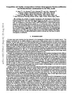
Since the maximum entropy solution has the property that the corresponding spectral density (3.24) lacks finite zeros, the speech becomes rather ”flat”. This is illustrated in Figure 3.1 where a true spectrum has been approximated by that of a 6th order maximum entropy filter. In Figure 3.2 we depict another solution, determined by our methods, of the same order but with appropriately chosen zeros.

10

0

-10

dB

-20

-30

-40

-50

-60

0

0.2

0.4

frequency

0.6

0.8

1

Figure 3.2 As these examples illustrate, in many speech processing applications zeros are desired, and the question arises whether it is possible to assign zeros arbitrarily and while still satisfying the interpolation condition. In view of (3.15) and (2.21), Georgiou’s result (Theorem 2.1) answers this question in the affirmative, even though the question of uniqueness had been left open. However, a computational procedure is needed. To this end, Georgiou [29] and Kimura [42] independently observed that the formula (3.22) could be generalized to 1 ψn (z) + α1 ψn−1 (z) + · · · + αn ψ0 (z) (3.26) 2 ϕn (z) + α1 ϕn−1 (z) + · · · + αn ϕ0 (z) 1 = + c1 z −1 + c2 z −2 + · · · + cn z −n + . . . , (3.27) 2 thus expressing v(z) in terms of the 2n parameters (α, γ), where α = (α1 , α2 , . . . , αn ) ∈ Rn and γ = (γ0 , γ1 , . . . , γn−1 ) ∈ Rn . In fact, it was shown in [29] and later also in [17] that the interpolation condition in (3.26) holds for all α, and consequently the Georgiou-Kimura parameterization v(z) =


(3.26) characterizes rationality but not positivity. We denote by subset of R2n for which v(z) is strictly positive real, and let

13

Pn the

Pn (γ) = {(α, γ) ∈ Pn | γ fixed} ⊂ Rn

be the positive real region for fixed covariance data. Of course, given the partial covariance data γ, the choice α = 0 is the maximum entropy solution, but in general it is very complicated to characterize those other α for which v(z) is positive real, i.e., to characterize the sets n (γ). For n = 1 the representation (3.26) takes the form

P

v(z) =

1 z + γ0 + α1 . 2 z − γ0 + α1

(3.28)

The strictly positive real region is the diamond depicted in Figure 3.3 below, and fixing the partial covariance data γ0 , the admissible α are the ones on the open interval in the figure. γ 1 1

−1

α

−1

Figure 3.3 Next, let us consider the case n = 2. Fixing the covariance data at γ0 = 12 and γ1 = 13 , we obtain v(z) =

1 z 2 − 23 z + 2 z 2 + 13 z +

1 3 1 3

+ α1 (z + 12 ) + α2 , + α1 (z − 12 ) + α2

(3.29)

and the region of positive real α = (α1 , α2 ) is as depicted in Figure 3.4. The higher-dimensional cases become much more complicated. While it is true that n (γ) is always diffeomorphic to Euclidean space [11], any good solution to the rational covariance extension problem would give such a parameterization in terms of familiar systems theoretic objects. In this direction, the possibility of parameterizing those filters which are positive real by arbitrarily prescribing the zeros of a modeling filter was suggested by Georgiou in Theorem 2.1 and his conjecture. Recently we proved an amplification of Georgiou’s conjecture that, for any desired choice of spectral

P

14


density zero structure, there is one and only one positive extension, i.e., one and only one modeling filter. This result was obtained by viewing a certain fast filtering algorithm as a nonlinear dynamical system defined on the space of positive real rational functions of degree less than or equal to n. It is then observed that filtering and interpolation induce complementary, or “dual” decompositions (or foliations) of this space. From this assertion about the geometry of positive real functions follows the first complete parameterization of all positive rational extensions [15]. This will be the topic of Sections 4–6.

α2

1

α1 1

Figure 3.4

4. The fast filtering algorithm: a dynamical system which computes spectral factors The connection between the Carathéodory function v(z) of a rational covariance extension and the corresponding modeling filter w(z) is through spectral factorization. More precisely, given a strictly positive real v(z), the modeling filter w(z) is the minimum phase solution of w(z)w(z −1 ) = v(z) + v(z −1 ).

(4.1)

If v(z) :=

1 b(z) , 2 a(z)

(4.2)

where a(z) and b(z) are monic Schur polynomials (2.19) and (2.20), we saw in Section 3 that w(z) = ρ

σ(z) , a(z)

(4.3)


15

where σ(z) is the Schur polynomial solution (3.14) of the polynomial spectral factorization problem ρ2 σ(z)σ(z −1 ) = d(z) :=

1 [a(z)b(z −1 ) + a(z −1 )b(z)]. 2

(4.4)

The spectral factorization problem (4.1) then amounts to determining σ(z) from a(z) and b(z). There is a well-known connection between spectral factorization and Kalman filtering that we shall exploit next. In fact, solving the spectral factorization problem by iterating the Riccati equation of Kalman filtering to steady state is a common procedure. Here we shall use the same idea but instead applied to a certain fast algorithm for Kalman filtering. We shall formulate the Kalman filtering problem in terms of covariance data or, equivalently, in terms of the Carathéodory function v(z). Defining g(z) :=

1 [b(z) − a(z)] = g1 z n−1 + g2 z n−2 + · · · + gn , 2

(4.5)

1 g(z) + , 2 a(z)

(4.6)

1 + h (zI − F )−1 g, 2

(4.7)

we may write v(z) = or, alternatively, v(z) =

where, without lack of generality, we have taken (F, g, h) in the observer canonical form       −a1 1 0 ··· 0 1 g1  −a2  0 1 · · · 0  0  g2   .. .. . . . g =   h =   F =  ... (4.8)  ..   ..  . ..  . .   . . −an−1 0 0 · · · 1 0 gn −an 0 0 ··· 0 and where prime ( ) denotes transpose. Sometimes it is convenient to write F = J − ah

(4.9)

where a is the column vector (a1 , a2 , . . . , an ) and J is the obvious shift matrix. Now, let w(z) be the corresponding modeling filter, and consider the stationary random sequence {y(t)}t∈Z obtained by passing white noise through the shaping filter u

y

white noise −→ w(z) −→

16


with transfer function w(z) or some other spectral factor of v(z) + v(z −1 ). Then the one-step predictor, i.e., the linear least squares estimate yˆ(t) of y(t) given y(0), y(1), . . . , y(t − 1), is generated by the Kalman filter x ˆ(t + 1) = F x ˆ(t) + k(t)[y(t) − h x ˆ(t)] yˆ(t) = h x ˆ(t)

(4.10)

where the gain k(t) can be determined via a matrix Riccati equation. Apparently less well-known is that the gain can also be determined via the fast algorithm a(t + 1) = g(t + 1) =

1 1−g1 (t) [a(t) + (I − J)g(t)] 1 1−g1 (t)2 [−g1 (t)a(t) + (J − g1 (t)I)g(t)]

a(0) = a g(0) = g (4.11)

consisting of 2n nonlinear first-order difference equations, in terms of which k(t) = a(t) + g(t) − a.

(4.12)

We say that it is “fast” since, for n > 1, 2n is less than the number 12 n(n+1) of scalar equations in the corresponding matrix Riccati equation. This algorithm is a version, appearing in [47], of the fast Kalman filtering algorithm introduced in [46]. (Also see [16] where these matters are reviewed.) It is also shown in [47] that the equality 1 rt [at (z)bt (z −1 ) + at (z −1 )bt (z)] = d(z) 2

(4.13)

t−1 is preserved along the trajectory of (4.11), where rt := k=0 [1 − g1 (t)2 ] and the monic polynomials at (z) and bt (z) := at (z) + 2gt (z) are formed from a(t) and b(t) := a(t) + 2g(t) as above, and that at (z) and bt (z) have all their zeros in the unit disc |z| < 1. An important property of the fast algorithm (4.11) is that the 2n parameters (a, g) of the problem appear only in the initial conditions and not in the dynamical system, which is invariant under parameter changes. In fact, the algorithm updates the parameters and can therefore be regarded as an iteration in parameter space. Moreover, the algorithm makes sense also for initial data (a, g) which does not correspond to a positive real v(z). We now express this dynamical system in the Georgiou-Kimura coordinates. In fact, the parameterization (3.26) can be given a nice geometric interpretation as a birational diffeomorphic change of coordinates in the strictly positive real region

P = {(a, g) ∈ R2n | v(z) is strictly positive real}


17

[18]. In fact, the Georgiou-Kimura parameterization yields a(z) = ϕn (z) + α1 ϕn−1 (z) + · · · + αn ϕ0 (z) (4.14) b(z) = a(z) + 2g(z) = ψn (z) + α1 ψn−1 (z) + · · · + αn ψ0 (z) where the Szegö polynomials {ϕn (z)}n0 and {ψn (z)}n0 are determined from γ := (γ0 , γ1 , . . . , γn−1 ) via the Szegö recursions (2.8) and (2.11). The fast filtering algorithm (4.11) can now be reformulated as a nonlinear dynamical system in (α, γ)-space [18]. More precisely, if (α, γ) ∈ n and the maps A, G : Rn → Rn×n are defined as

P

   A(γ) =   

1 2 1−γn−1

0 .. . 0

γn−1 γn−2 2 2 (1−γn−1 )(1−γn−2 ) 1 2 1−γn−2

··· ··· .. . ···

.. . 0

 γn−1 γ0 2 (1−γn−1 )···(1−γ02 ) γn−2 γ0  2 (1−γn−2 )···(1−γ02 ) 

 (4.15)  

.. .

1 1−γ02

and 

0 0 .. .

   G(α) =    0 −αn

1 0 .. .

0 1 .. .

··· ··· .. .

0 −αn−1

0 −αn−2

··· ···

then the dynamical system α(t + 1) = A(γ(t))α(t), γ(t + 1) = G(α(t + 1))γ(t),

0 0 .. .



   ,  1  −α1

α(0) = α γ(0) = γ

(4.16)

(4.17)

initiated at (α, γ) evolves on the invariant manifold defined by (4.13). In fact, the preserved pseudo-polynomial (4.13) yields, after change of coordinates and identification of coefficients of like powers in z, n + 1 equations in the 2n+1 variables {α(t), γ(t), rt } which, upon elimination of rt by dividing the last n equations by the first, in turn yields n integrals fi (α(t), γ(t)) = κi

i = 1, 2, . . . , n

(4.18)

for the dynamical system (4.17), where κ1 , κ2 , . . . , κn are constants, which can be determined from the initial conditions (α, γ). Moreover, γ(t) is updated by shifting so that γk (t) = γt+k .

(4.19)

18


P P

Theorem 4.1 ([18]). The strictly positive real region n is invariant under the dynamical system (4.17), which is globally convergent on n . More specifically, (α(t), γ(t)) tends to (α∞ , 0), where α∞ ∈ n (0) ⊂ Rn so that α∞ (z) = z n + α∞1 z n−1 + · · · + α∞n

P

(4.20)

P

is a monic Schur polynomials of degree n and n (0) is the equilibrium set. The global stable manifold s (α∞ , 0) of the equilibrium (α∞ , 0) is defined by (4.18) with κi = fi (α∞ , 0) for i = 1, 2, . . . , n.

W

A consequence of this theorem and (4.19) is that γt → 0

as t → ∞.

(4.21)

Therefore, since the Szegö polynomials ϕk (z) and ψk (z) become z k when the Schur parameters are zero, this implies in view of (4.14) that at (z) → α∞ (z)

and bt (z) → α∞ (z)

as t → ∞

(4.22)

in (4.13). Likewise, rt → r∞

as t → ∞,

(4.23)

and consequently the pseudo-polynomial d(z) corresponding to the stable manifold s (α∞ , 0) becomes

W

d(z) = r∞ α∞ (z)α∞ (z −1 ).

(4.24)

Therefore, evaluating (4.13) for t = 0 and noting that r0 = 1 we have 1 [a(z)b(z −1 ) + a(z −1 )b(z)] = r∞ α∞ (z)α∞ (z −1 ), 2

(4.25)

which should be compared with the spectral factorization equation (4.4). Consequently, the required spectral factor is w(z) =

√

r∞

α∞ (z) , a(z)

(4.26)

where α∞ (z) is obtained from the limit of the dynamical system and r∞ is easiest determined from (4.25) by identifying coefficient of like power in z.


19

5. The complementary foliations In this section we shall investigate the geometry of the strictly positive real region, i.e. the open subset ⊂ R2n of (α, γ) such that

P

v(z) =

1 ψn (z) + α1 ψn−1 (z) + · · · + αn ψ0 (z) 2 ϕn (z) + α1 ϕn−1 (z) + · · · + αn ϕ0 (z)

(5.1)

is strictly positive real, where {ϕk (z)}n0 and {ψk (z)}n0 are the Szegö of the first and second type respectively corresponding to the covariance data γ. Similarly, as before let

Pn (γ) = {(α, γ) ∈ Pn | γ fixed} ⊂ Rn

(5.2)

be the strictly positive real region for fixed covariance data. Geometrically, the decomposition 1 : n = n (γ)

F

P

P

(5.3)

γ

is an important example of what is known as a foliation of the open manifold n . Intuitively, a foliation is a decomposition of a manifold into disjoint connected submanifolds, called leaves, with the additional property that in the neighborhood of any point the leaves vary in a sufficiently smooth way. More precisely, a foliation of dimension m on a smooth manifold M of dimension n is a partition of M into a family of disjoint, connected m-dimensional submanifolds Lβ , called the leaves of the foliation, such that (i) M = ∪β Lβ , (ii) each point x ∈ M has a Euclidean neighborhood U and coordinates (x1 , ..., xn ) for which the equations

P

F

x1 = 0,

x2 = 0,

...,

xn−m = 0

define the connected components of the nonempty intersections U ∩ Lβ . In fact, it was shown in [11] that n (γ) is diffeomorphic to Euclidean space and is therefore connected. With this in mind, we note (see [7]) that the Kimura-Georgiou parameterization shows that this decomposition is sufficiently regular to define a foliation 1 of n into the leaves n (γ) (see [15]. In Section 4 we showed that for any (α, γ) ∈ n the dynamical system (4.17) converges to a limit (α∞ , 0) ∈ n along the stable manifold s (α∞ , 0). As proved in [15], the decomposition of n as a union of the global stable manifolds s (α∞ , 0) defines a second foliation s (α∞ , 0) (5.4) 2 : n =

P

F

P

P

W

W

F

P

P

P

α∞ ∈ (0)

P

P

P

W

of n . In the special case n = 1, Figure 5.1 depicts the global stable manifold s (α∞ , 0) at ( 13 , 0) as a subset of 1 . Also depicted is 1 ( 12 ).

W

P

P

20


F

F

As Figure 5.1 suggests the leaves of the foliations 1 and 2 are transverse, i.e. at a point of intersection of the leaves of these two foliations the corresponding tangent spaces are complementary subspaces. Indeed, using the characterization of the tangent spaces to the stable manifold s (α∞ , 0) developed in [18], in [15] we proved that the intersection of s (α∞ , 0) with n (γ) is in fact always transverse. In such a case, one says that two foliations are complementary.

W

P

W

γ s

W (σ,0)

−1

P1

1

P1(γ)

α σ

α

1

−1

Figure 5.1

P

Theorem 5.1. The positive real region n is connected and is foliated by the stable manifolds s (α∞ , 0) of the equilibrium set n (0). The set n is also foliated into leaves given by the submanifolds n (γ). Moreover, these foliations are complementary.

W

P

P

P

P

Consequently, there are two complementary foliations of n , one indexed by the partial covariance data and one by the zero polynomial of the modeling filter. Theorem 5.1 suggests that, given a partial covariance sequence and a stable zero polynomial, there is a unique solution of the rational covariance problem represented by the intersection between the corresponding leaves of the foliations 1 and 2 . The fact that these foliations are complementary says that this uniqueness does occur to first order, in the following sense.

F

F

Corollary 5.2. For each (λ, α) ∈ R+ × of fγ is nonsingular.

Pn (γ), the Jacobian matrix Jac fγ

In fact, in [15] Corollary 5.2 formed the basis for a degree theoretic argument which demonstrated that to any point σ in n (0), there is one

P


21

P

and only one α such that (α, γ) ∈ n (γ). This α defines a modeling filter w(z) having the zeros of σ(z). It is interesting to note that, conversely, any α such that (α, γ) ∈ n (γ) determines a Schur polynomial σ(z), which can be computed via the convergence of the dynamical system (4.17) with initial condition determined by (α, γ). In fact, the dynamical system defines a map

P

g:

Pn (γ) → Pn (0)

(5.5)

sending a strictly positive real choice of the parameters α in the GeorgiouKimura parameterization (5.1) to the corresponding choice of stable zeros g(α) = σ.

(5.6)

As an illustration in the case n = 2 , Figure 5.2 depicts the connected open submanifolds 2 (γ) and 2 (0), the latter corresponding to the monic Schur polynomials in 2 , for γ = (1/2, 1/3). These sets form the domain and codomain of the function g sending α to σ .

P

P

S

σ2

α2

1

1

σ1

α1 1

1

Figure 5.2 In the next section we shall sketch a new proof that the function g is a diffeomorphic bijection, using a theorem of Hadamard to show that the rational covariance extension problem is well-posed. 6. A complete parameterization of all rational covariance extensions As pointed out above, the maximum entropy solution gives rise to a rational spectral density with no finite zeros, and hence a modeling filter with all zeros in the origin. In many applications, it turns out to be important to be able to design filters with prescribed zeros and which shape processes with observed correlation coefficients. The important question as to which zeros can be prescribed, and in which manner, has been a limiting factor in filter design. In order to address this issue, Georgiou [29] launched an investigation of which zeros could be prescribed using degree theory a tool for studying the

22


existence of solutions to nonlinear equations. In 1983, he proved that any Schur polynomial is possible as the numerator of a modeling filter which interpolated the given covariance data (Theorem 2.1) and conjectured that there is a unique zero polynomial to each rational covariance extension of degree at most n. In practice, however, we would require more, e.g., that the solutions should depend continuously in the problem data, so that small variations in problem data would give rise to small variations in the solution. In [15] we proved Georgiou’s conjecture in this stronger form as a corollary of Theorem 5.1, which, among other things, provides a complete (and analytic) parameterization of all rational covariance extensions of degree at most n. Theorem 6.1 ([15]). Suppose one is given a finite sequence of real numbers c0 , c1 , c2 , . . . , cn

(6.1)

which is positive in the sense that the Toeplitz matrix   c1 c2 ... cn c0  c1 c0 c1 . . . cn−1    Tn =  . . . ..  .. .. ..  .. . .  cn cn−1 cn−2 . . . cn

(6.2)

is positive definite. Then, to each Schur polynomial σ(z) = z n + σ1 z n−1 + · · · + σn ,

(6.3)

there corresponds a unique Schur polynomial a(z) = z n + a1 z n−1 + · · · + an

(6.4)

such that, for some suitable uniquely defined positive number ρ, w(z) = ρ

σ(z) a(z)

(6.5)

satisfies the interpolation condition w(z)w(z −1 ) = 1 +

∞

cî (z k + z −k ) ;

cî = ci

for

i=k

i = 1, 2, . . . , n (6.6)

Moreover, this one-one correspondence is an analytic diffeomorphism. We begin by noting that Theorem 6.1 would follow if we could prove that the function fγ : R+ × n (γ) → n , given by

P

fγ (λ, α) =

D

1 λ[a(z)b(z −1 ) + a(z −1 )b(z)] 2

(6.7)


23

is a diffeomorphism. Here a(z) and b(z) depend on α ∈ Rn via (4.14), and n is the space of pseudo-polynomials

D

d(z) = d0 + d1 (z + z −1 ) + · · · + dn (z n + z −n ),

(6.8)

of degree at most n which are positive on the unit circle. In fact, if fγ is a diffeomorphism for all γ satisfying the Schur condition (2.13), then it is in particular a diffeomorphism for γ = 0 so that the map f0 : R+ × n (γ) → n defined via f0 (µ, σ) = µσ(z)σ(z −1 )

P

D

is a diffeomorphic bijection. Then the commutative diagram

R+ × Pn (0)

h

−→

f0

Dn

R+ × Pn (γ)

fγ−1

defines a homeomorphic bijection h under which 1 λ[a(z)b(z −1 ) + a(z −1 )b(z)] = µσ(z)σ(z −1 ). 2 Setting ρ2 := µ/λ, this is equivalent to 1 b(z) σ(z) σ(z −1 ) 1 b(z −1 ) + = ρ2 , −1 2 a(z) 2 a(z ) a(z) a(z −1 ) where 1 b(z) 1 = + c1 z + · · · + cn z −n + . . . 2 a(z) 2 interpolates the given partial covariance sequence so that w(z) = ρ

σ(z) a(z)

is a modeling filter. Therefore, Theorem 6.1 would follow. A new proof of the fact that fγ is a diffeomorphic bijection can in fact be based on a theorem by Hadamard [33, 34, 35], as we shall now see. Hadamard formalized the concept of well-posedness of problems described by maps between Euclidean n-spaces was as follows. For such an f , the problem of finding solutions to f (x) = y is said to be well-posed provided f is (i) surjective, (ii) injective, and (iii) has a continuous inverse. The criterion for well-posedness given by Hadamard reposes upon a property of maps which reflects the existence of a priori bounds on the size of solutions, given bounds on the size of the problem data. Topologically, this can be expressed in terms of properness. Recall that a function f : Rn → Rn is said to be proper if, and only if, f −1 (K) is compact for every compact

24


K. In these terms, there are several related criteria for well-posedness, the earliest such result being in essence a global inverse function theorem. Theorem 6.2 (Hadamard’s Theorem). Suppose f : Rn → Rn is a C 1 map. If f is proper and satisfies det Jac f = 0 for every x ∈ Rn , then f is a diffeomorphism onto Rn . Hadamard’s Theorem can be proven by either degree theory or by the theory of covering spaces [5]. For these reasons, there are also extensions of this theorem to classes of spaces and maps to which either of these theories apply. However, one should also expect the topology of more general spaces to complicate the conclusion of the analogues of this basic theorem. As an example, consider the map f defined on the unit circle S 1 in the complex plane, with the unit circle as its range, defined via f (z) = z 2 . The map f satisfies all the hypotheses in Hadamard’s Theorem, except that of having Euclidean spaces for it domain and range. However, f is not a diffeomorphism but rather exhibits its domain as a double covering of its range. In our application of Hadamard’s Theorem it is of course essential that the domain and range be Euclidean spaces. To illustrate this point further, we shall consider as a preliminary example the question of whether fγ is a diffeomorphism in the case, γ = 0, which is the problem of spectral factorization. More precisely, given a symmetric pseudo-polynomial d(z) = d0 + d1 (z + z −1 ) + · · · + dn (z n + z −n ),

(6.9)

of degree at most n, which is positive on the unit circle, find a stable polynomial a(z) of degree n, i.e., a polynomial a(z) = a0 z n + a1 z n−1 + · · · + an ,

a0 > 0

(6.10)

having all its roots strictly inside the unit circle, such that a(z)a(z −1 ) = d(z).

(6.11)

Such spectral factors a(z) are of course unique if they exist. In fact, a(z) has n roots each of which is either zero, and hence canceling with a(z −1 ), or a root of d(z). Conversely, a root of d(z) located in the open unit disc is nonzero and a root of a(z). Consequently, all polynomials satisfying (6.11) have the same roots. Then the a0 must also be the same, and hence the polynomials are identical. Although simple to see in a more direct way, to illustrate our point of view we shall give a topological proof for existence of a solution to (6.11). Lemma 6.3. The space morphic with Rn+1 .

Zn of all stable polynomials of degree n is diffeo-


25

Sn the space of Schur polynomials, that is the space of

Proof. Denote by monic polynomials

b(z) = z n + b1 z n−1 + · · · + bn ,

(6.12)

Z

which have all its roots strictly inside the unit circle. The space n of all stable polynomials of degree n is diffeomorphic to the product R+ × n via the mapping ϕ : a(z) → (a0 , a(z)/a0 ). By identifying a monic polynomial with its roots, the space n may be identified with the space of real divisors of order n in the open unit disc, where by a real divisor of order n we mean a self-conjugate, unordered sets of n points. Therefore, by identifying the open unit disc with the complex plane via a diffeomorphism which preserves conjugation, one can also identify the space of all real divisors of order n in the open unit disc with the space of all real divisors of order n in the complex plane, i.e., with the space of all real monic polynomials of degree n. In this way, n is diffeomorphic to Rn . Therefore, n is diffeomorphic with a product of Euclidean spaces and hence diffeomorphic with Rn+1 .

S

S

S

Z

Z

Zn → Wn from the vector Wn of symmetric pseudo-

For any a ∈ n , define the operator S(a) : space n into the n + 1-dimensional vector space polynomials of degree at most n via

Z

S(a)b =

1 [a(z)b(z −1 ) + a(z −1 )b(z)]. 2

(6.13)

In view of the unit circle version of Orlando’s formula [27], S(a) is nonsingular for all a ∈ n . (Also see, e.g., [24] where a determinantal expression is given.) Let n ⊂ n be the space of pseudo-polynomials (6.9) which are positive on the unit circle. Then for any d ∈ n , S(a)b = d uniquely defines b(z) and hence b = S(a)−1 d ∈ n . a strictly positive real function v(z) = 12 a(z) The operator G : n → n defined by

D

Z

Z

W

D

Z

Z

Ga = S(a)−1 d

(6.14)

is an involution, i.e., G2 a = a. In fact, in view of (6.13), Ga = b and Gb = a. By Smith’s Theorem [6], an involution which maps a Euclidean space into itself has a fixed point, and therefore there exists a solution a ∈ n to (6.11) for all d ∈ n .

Z

D

Remark 6.4. The existence of spectral factors can of course, be proven in a much more straight-forward manner. On the other hand, polynomial spectral factorization is the simplest form of the rational covariance extension problem and also illustrates one of the key points to which we shall now turn. That is, our proof relies heavily on the fact that n is homeomorphic to Rn+1 since on many non-Euclidean spaces there exist involutions without fixed points.

Z

26


We now proceed with the proof of Theorem 6.1 using the global inverse function theorem, Theorem 6.2. We note that fγ is easily shown to be proper, as in [15, Lemma A.2]. Next, the duality between filtering and interpolation implies that for each (λ, α) ∈ R+ × n (γ) the matrix Jac fγ is in fact nonsingular, as we noted in Corollary 5.2. Finally, it remains to check that the domain and range of fγ are diffeomorphic to Euclidean space. By spectral factorization, the open manifold n is diffeomorphic to n , which we know is Euclidean by Lemma 6.3. Thus, it remains to prove that the domain of fγ is Euclidean. The fact that the open manifold R+ × n (γ) is diffeomorphic to Euclidean space follows of course from the same assertion about n (γ). That n (γ) is diffeomorphic to Euclidean space was shown in [11] using the BrownStallings criterion [55], which asserts that an n-manifold is diffeomorphic to Euclidean n-space if and only if every compact subset has a Euclidean neighborhood. Very briefly, the proof uses two facts. The first is that to say v(z) is positive real is to say that for any µ ∈ C+ the polynomial b(z) + µa(z) has all its roots in the unit disc. This allows one to pass to a problem about compact sets of divisors in the unit disc. The second tool is a general method for recognizing Euclidean spaces of polynomials from their divisors: If U is a self conjugate open subset of C with a simple, closed, rectifiable, orientable curve as boundary, then the space of all monic real polynomials with all of their roots lying in U is diffeomorphic to Rn . The proof, of course, follows the proof of Lemma 6.3, mutatis mutandis. This concludes the proof of Theorem 6.1.

P

D

Z

P

P

P

Caveat. This solution to the rational covariance extension problem expresses the choice of free parameters in familiar systems theoretic terms, viz. the numerator of the resulting modeling filter. One might imagine that a similar situation holds if one were to first choose the pole polynomial. However, although the zeros of the modeling filter can be chosen arbitrarily, this is not the case for the poles, as can be seen from the following simple counter example. Counter Example. Consider the partial covariance sequence (1, c1 ) = (1, 12 ). Then n = 1 and γ0 = 12 . Now suppose we would like to chose the stable pole polynomial a(z) = z + a1 with a1 = 34 . Then it follows from (3.28) that α1 = a1 + γ0 = 54 . However, as can be seen from Figure 3.3, the point (α, γ) = ( 54 , 12 ) does not belong to the strictly positive real region 1 . This can also be seen from the fact that b(z) = z + 74 , which is not a Schur polynomial.

P

7. Minimality An important and partially open question in partial stochastic realization theory is to find the rational covariance extension of minimum McMillan


27

degree. More precisely, given a partial covariance sequence 1, c1 , c2 , . . . , cn ,

(7.1)

find an infinite extension cn+1 , cn+2 , . . . with the property that the corresponding positive real function v(z) =

1 + c1 z −1 + c2 z −2 + c3 z −3 + . . . 2

has minimum degree. This degree is called the positive degree of the partial covariance sequence (7.1). It is easy to see, and follows readily from classical stochastic realization theory, that the degree of the corresponding modeling filter w(z) is the same as that of v(z). If p < n, the polynomials a(z), b(z) and σ(z) thus must have common factors. This is equivalent to finding the minimum triplet (F, g, h) of matrices such that (i) (ii)

h F k−1 g = ck for k = 1, 2, . . . , n and v(z) is strictly positive real,

i.e. the matrices F, g and h having the dimensions p × p, p × 1 and p × 1 respectively with the smallest possible p such that (i) and (ii) are satisfied. This p is precisely the positive degree of (7.1). If the positivity requirement (ii) is removed, the problem reduces to the much simpler deterministic partial realization problem [39, 40, 31], The corresponding degree, the algebraic degree of (7.1), is of course smaller or equal to the positive degree p. Nevertheless, they are often confused in the literature. As a starting point for studying the positive degree of a partial covariance sequence, it would be helpful to be able to compute the degree of the positive real rational function which we know corresponds to any fixed choice of zero polynomial σ(z). To this end, we shall next introduce a Riccati-type equation, called the Covariance Extension Equation, which is formulated in terms of the partial covariance data and a choice of desired modelingfilter zeros [14, 12, 13]. This is a nonstandard Riccati equation the positive semidefinite solutions of which parameterize the solution set of the rational covariance extension problem in terms of the partial covariance sequence and the zeros of the desired modeling filter. While it is interesting in its own right, in the present setting of partial covariance data, the Covariance Extension Equation (CEE) replaces the usual algebraic Riccati equation of stochastic realization theory required when the covariance data is complete. It is convenient to represent the given covariance data 1, c1 , c2 , . . . , cn in terms of the first n coefficients in the expansion zn z n + c1 z n−1 + · · · + cn

= 1 − u1 z −1 − u2 z −2 − u3 z −3 − . . .

(7.2)

28


about infinity and to define 



u1  u2    u= .   ..  un





0 u1 u2 .. .

   U =   un−1

0 u1 .. . un−2

   .  

..

. ···

u1

(7.3)

0

Likewise, we may collect the coefficients of the desired zero polynomial σ(z) = z n + σ1 z n−1 + · · · + σn , in the matrices   σ1  σ2    σ =  . ,  ..  σn



−σ1 −σ2 .. .

   Γ=  −σn−1 −σn

1 0 .. .

0 1 .. .

··· ··· .. .

0 0

0 0

··· ···

 0 0  ..  .  1 0

(7.4)

  1 0   and h =  .  . (7.5)  ..  0

The Covariance Extension Equation is given in terms of these parameters as P = Γ(P − P hh P )Γ + (u + U σ + U ΓP h)(u + U σ + U ΓP h) (7.6) where the n × n matrix P is the unknown. Our principal result concerning the CEE concerns existence and uniqueness of the positive semi-definite solution, similar in spirit to the classical existence and uniqueness theorems for the Riccati equations arising in filtering and control, and the connection of this solution to the corresponding modeling filter (7.7). This, of course, is of considerable independent interest in partial stochastic realization theory. The following theorem was first presented in [12, 13] and proved in [14]. Theorem 7.1. Let (1, c1 , · · · , cn ) be a given positive partial covariance sequence. For every Schur polynomial σ(z), there exists a unique positive semidefinite solution P of the Covariance Extension Equation satisfying h P h < 1, to which in turn there corresponds a unique modeling filter w(z) = ρ

σ(z) , a(z)

(7.7)

for which the denominator polynomial a(z) = z n + a1 z n−1 + · · · + an ,

(7.8)

a = (I − U )(ΓP h + σ) − u

(7.9)

is given by


29

and ρ ∈ (0, 1] is a real number given by ρ = (1 − h P h)1/2 .

(7.10)

All modeling filters are obtained in this way. Moreover, the degree of w(z), and hence that of v(z), equals the rank of P . From the last statement of Theorem 7.1 we see that the degree of any rational covariance extension, and hence the positive degree of a partial covariance sequence, is connected to the corresponding solution of the Covariance Extension Equation. In fact, one can derive the following corollary of Theorem 7.1. Corollary 7.2. The positive degree of the partial covariance sequence (7.1) is given by p = min rank P (σ),

Sn

σ∈

(7.11)

where P (σ) is the unique solution of the Covariance Extension Equation corresponding to (7.1) and the zero polynomial σ, and the minimization is over the space n of all Schur polynomials of degree n. The modeling filter corresponding to a minimizing σ is a minimal partial stochastic realization of (7.1).

S

This corollary does not of course provide us with an applicable algorithm for determining the positive degree or a minimal rational covariance extension, but it does explain the connection to the CEE. Since positive degree has often been confused with algebraic degree,

and since the algebraic degree of sequences (7.1) has the generic value n+1 , it 2 is important to investigate whether there is a generic positive degree and, if so, what it is. To this end, represent the covariance data as a vector   c1  c2    c :=  .  ∈ Cn ⊂ Rn ,  ..  cn where Cn is the set of c with positive Toeplitz matrix. Recall that a subset of Rn is semialgebraic provided it can be defined by a finite number of polynomial equations, inequations, and inequalities. For example, Cn is a semialgebraic subset of Rn , being defined by polynomial inequalities. A subset of Rn is algebraic provided it can be defined by a finite number of polynomial equations. Finally, a property of points in Rn is said to be generic if the set of points which enjoy this property is nonempty, with its complement being contained in an algebraic set.

30


Theorem 7.3. Let p be any integer such that n2 ≤ p ≤ n. Then the subset of c ∈ Cn having positive degree p is a semialgebraic set containing a nonempty open subset of Rn . Consequently, the positive degree has no generic value. The proof of this theorem, which has important consequences for socalled subspace identification algorithms [61, 51], can be found in [14]. We shall now illustrate this result by considering the special case n = 2. Instead of using the representation c = (c1 , c2 ) for the covariance data, we shall use (γ0 , γ1 ), which of course is equivalent. It is easy to check that p = 0 if and only if γ0 = γ1 = 0, p = 1 if and only if |γ1 |
2 the situation is more complicated, but we have a sufficient condition for the positive degree p to be strictly less than n, which is similar to (7.12).


31

Corollary 7.4. Suppose n ≥ 2. Any partial covariance sequence satisfying the condition |γn−1 |