Jan 15, 2015 - HAL Id: hal-01103720 https://hal.archives-ouvertes.fr/hal-01103720. Submitted ...... vibrated hopper does show the bi-valued distribution [21].
On-and-off dynamics of a creeping frictional system Baptiste Blanc, Jean-Christophe G´eminard, Luis Pugnaloni
To cite this version: Baptiste Blanc, Jean-Christophe G´eminard, Luis Pugnaloni. On-and-off dynamics of a creeping frictional system. the european physical journal, 2014, 37, pp.112. .
HAL Id: hal-01103720 https://hal.archives-ouvertes.fr/hal-01103720 Submitted on 15 Jan 2015
HAL is a multi-disciplinary open access archive for the deposit and dissemination of scientific research documents, whether they are published or not. The documents may come from teaching and research institutions in France or abroad, or from public or private research centers.
L’archive ouverte pluridisciplinaire HAL, est destin´ee au d´epˆot et `a la diffusion de documents scientifiques de niveau recherche, publi´es ou non, ´emanant des ´etablissements d’enseignement et de recherche fran¸cais ou ´etrangers, des laboratoires publics ou priv´es.
EPJ manuscript No. (will be inserted by the editor)
On and off dynamics of a creeping frictional system Baptiste Blanc1 , Jean-Christophe G´eminard1 , and Luis A. Pugnaloni2 1
2
Universit´e de Lyon, Laboratoire de Physique, Ecole Normale Sup´erieure de Lyon, CNRS, 46 All´ee d’Italie, 69364 Lyon cedex 07, France. Departamento de Ingenier´ıa Mec´ anica, Facultad Regional La Plata, Universidad Tecnol´ ogica Nacional, Av. 60 esq. 124, 1900 La Plata, Argentina. Received: January 15, 2015/ Revised version: date Abstract. We report on the dynamics of a model frictional system submitted to minute external perturbations. The system consists of a chain of sliders connected through elastic springs that rest on an incline. By introducing cyclic expansions and contractions of the rest length of the springs, we induce the reptation of the chain. Decreasing the amplitude of the perturbation below a critical value, we observe an intermittent creep regime characterized by alternated periods of reptation (flowing state) and rest (quiescent state). A further decrease of the perturbation leads to the disappearance of the reptation. The width of the transition region between the continuous creep and the full stop (i.e., the range of excitation amplitudes where the intermittent creep is observed) is shown to depend on the difference between the static (µs ) and the dynamic (µd ) friction coefficients. For µs = µd the intermittent creep is not observed. Studying the statistical features of the intermittent creep regime for any given perturbation amplitude, we find that the time the system resides in each state (flowing or quiescent) suggests that: (i) reptation events are uncorrelated, and (ii) rest events are history dependent. We show that this latter history dependency is consistent with the aging of the stress state inside the chain of sliders during the quiescent periods. PACS. 46.55.+d Tribology and mechanical contacts – 65.40.De Thermal expansion; thermomechanical effects – 62.20.Hg Creep.
1 Introduction Granular materials present interesting and unusual physical properties [1]. Most of these properties are caused by the dissipative character of the grain–grain interaction, chiefly the peculiarities of solid friction. At the grain scale, solid friction presents a sharp transition from the static friction coefficient µs to the dynamic friction coefficient µd . In some studies [2], a viscous damping force is used to smooth this transition and take the limit to the continuum. However, in the realm of granular materials, for the scale of interest set by the characteristic size of the grains, the effect of such discontinuity in the friction coefficient becomes measurable and of practical importance. This has important effects on very slow processes in dense granular matter, such as creep, where the sudden change of the interaction on a single contact can trigger noticeable rearrangements in the system. Two practical examples of these slow processes are clogging–unclogging during granular flow, stimulated by vibrations [3], through small orifices [4, 5], and the compaction of granular columns under thermal cycling [6, 7]. When grains flow through a small orifice, the flow may halt due to clogging [8, 9]. The use of vibrations can break blocking arches and stimulate the flow [3]. Nevertheless, even with a sustained energy input, relatively stable arches
can stop the flow for long periods of time. This induces intermittency in the flow with a distribution of blockage time that depends on the amplitude of the vibration [4]. In a similar manner, oscillations of room temperature can be used to induce minute and slow perturbations on a granular column. Above a critical amplitude of the temperature variations, the system undergoes continuous rearrangements that lead to compaction. However, at small amplitudes, the assembly compacts intermittently, with only some thermal cycles leading to rearrangements [6, 7]. We have recently considered a simple model that takes all the basic ingredients involved in the phenomena mentioned above [10]. Briefly, the model consists of a chain of frictional sliders, connected by elastic springs, that lies on an incline. When subjected to periodic “temperature changes”, simulated by changes in the rest length of the springs, the chain creeps downwards. We showed, assuming µs = µd , that under periodic temperature variations the chain creeps downwards every cycle only when the thermal amplitude is larger than a critical value. Analytical estimates of the critical amplitude and of the creep velocity above this thermal amplitude showed good agreement with numerical simulations of the model. Preliminary observations also indicated that, for a finite number of sliders and µs 6= µd , the system exhibits a complex dy-
2
Baptiste Blanc et al.: On and off dynamics of a creeping frictional system
At rest, the contact between any slider and the incline is characterized by a unique static frictional coefficient µs such that each slider, initially at rest, starts moving if
1 2 i N-1 N
|fn+1→n + fn−1→n + mg sin α| > µs mg cos α.
α
x Fig. 1. Sketch of the system.
namics in the vicinity of the transition between continuous creep and full stop. In this paper, we focus on this phenomenon and show that for µs 6= µd an intermittent creep regime (on and off dynamics), which shows alternated periods of creep (on state) and rest (off state), appears in the vicinity of the transition. We characterize this regime by studying the survival time of the rest and creep periods and consider the effect of the difference between µs and µd . This type of behavior cannot be observed in models that take the continuum limit for the frictional interaction [11,12]. We will discuss that the discontinuity in the friction force is key to the complex spatio-temporal dynamics observed.
2 The model 2.1 Description The system (total mass M ) consists of a series of N identical sliders of mass m = M/N connected through (N − 1) identical springs (massless, stiffness k). The sliders are in frictional contact with an incline which makes an angle α with the horizontal (Fig. 1). They are subjected to the forces due to the springs, to their own weight mg (where g denotes the acceleration due to gravity) and to the reaction force from the incline (including the frictional force). The aim of the present study is to account for the dynamics of the system induced by simulated temperature changes. To do so, we consider that the natural length of the springs, l, depends linearly on the temperature T according to: � � l(T ) = l0 1 + κ(T − T0 ) (1) where κ stands for the thermal expansion coefficient of the material the springs are made of and l0 for the natural length of the springs at T0 . In accordance, the total length of the system at T0 , in absence of internal stress, is L = (N − 1) l0 . We further assume, for the sake of simplicity, that the stiffness k does not depend on the temperature and that the substrate does not dilate. Thus, at the temperature T , the force due to the spring, exerted by the slider (n + 1) on the slider n is: fn+1→n = −k [xn − xn+1 − l(T )]
(2)
where xn denotes the position of the slider n on the incline. From now on, the x-axis is oriented downwards, α is positive and the first slider is the upper one (Fig. 1).
(3)
At the boundaries of the system, f0→1 = 0 (n = 1) and fN +1→N = 0 (n = N ). Furthermore, we assume that the frictional contact is associated with a single, constant, dynamical frictional coefficient, µd (< µs ), when the slider is in motion. If the slider n is in motion, subjected to the associated dynamical frictional force, fd,n ≡ −µd mg cos α sgn(x˙ n )
(4)
where x˙ n denotes the velocity and sgn the sign function [sgn(u) = 1 if u > 0 and sgn(u) = −1 if u < 0]. When the mechanical system is submitted to temperature changes, some sliders initially at rest start moving if the length l(T ) exceeds a value such that condition Eq. (3) is satisfied for, at least, one slider. As a consequence, one or more sliders move and come back to rest. Such event constitutes, by definition, a mechanical rearrangement of the system. At this point, it is interesting to consider two characteristic times. On the one hand, due to its thermal inertia, the system exhibits a thermal characteristic time τth which limits the dynamics of the temperature changes and, thus, of the thermal dilations. In practice, for a macroscopic system whose typical size L ranges from a few millimeters to centimeters, τth ranges from seconds to hours. On the other hand, the dynamics of the mechanical p system is characterized by the typical time scale τdyn = m/k. In practice, assuming that the springs account for the elasticity of a solid block, one can consider τdyn ∼ L/cs , where cs stands of the speed of sound in the material the macroscopic solid is made of. For a typical size L, ranging from a few millimeters to centimeters and usual values of cs (about a few kilometers per second), we estimate τdyn ∼ 10−6 − 10−5 s, thus much smaller than τth . Hence, we consider that l(T ) is constant during the mechanical rearrangements which are, in practice, much faster than the temperature variations. It is worth mentioning that similar models have been used to study the statistical properties of earthquakes [13], to consider self organized criticality in mechanical systems [14] and to discuss fluctuation dissipation relations in dissipative dynamical systems in stationary regimes [15]. This model has also been used as a base for recent studies focusing on the dynamics of the onset of frictional interfaces [16–18]. In contrast with our approach to induce perturbations cyclically in all the springs, these previous works focused on driving the system by an external force acting at one end of the chain. 2.2 General system of equations 2.2.1 Mechanical system First, we write the differential equation governing the position xn of the slider n, when it is in motion. Introducing
Baptiste Blanc et al.: On and off dynamics of a creeping frictional system
the thermal dilation θ ≡ κ (T − T0 ) and the dimensionless 2 variables t˜ ≡ t/τdyn and x ˜ ≡ x/(g τdyn ), we have: ¨˜1 = −[˜ x x1 − x ˜2 + (1 + θ) ˜l0 ] −µd sgn(x ˜˙ 1 ) cos α + sin α
(n = 1) ,
¨˜n = −[2 x x ˜n − (˜ xn+1 + x ˜n−1 )] ˙ −µd sgn(x ˜n ) cos α + sin α
(n 6= 1, N ) , (6)
¨˜N = −[˜ x xN − x ˜N −1 − (1 + θ) ˜l0 ] −µd sgn(x ˜˙ N ) cos α + sin α
(n = N ) ,
(5)
(7)
2 where, in accordance, we defined ˜l0 ≡ l0 /(g τdyn ). Second, we recall that the slider n, if at rest, starts moving if the condition Eq. (3) is satisfied. Thus, using the dimensionless variables, we can write
|˜ x2 − x ˜1 − (1 + θ) ˜l0 + sin α| > µs cos α, |˜ xn+1 + x ˜n−1 − 2 x ˜n + sin α| > µs cos α, |˜ xN −1 − x ˜N + (1 + θ) ˜l0 + sin α| > µs cos α,
(8) (9) (10)
where the conditions Eq. (8) and Eq. (10) apply for the slider 1 and N respectively and the condition Eq. (9) for any other slider n 6= 1, N .
3
ends when all the sliders are back to rest. All the sliders are then resting at the new positions x ˜k+1 n . The procedure is iterated by finding, in the same way, the next critical value of the dilation θc which leads, according to the conditions Eq. (8) to Eq. (10), to the next mechanical rearrangement. For each θc , a new static state of the system is found. The procedure stops when the next critical dilation θc is beyond θq+1 . The system then expe0 rienced k 0 rearrangements. The x ˜kn are then the positions of the sliders at t = tq+2 . The long-term behaviour of the system, after many temperature cycles, is assessed by iterating the whole procedure.
3 Results 3.1 The transition In [10], we predicted analytically that, far above a given amplitude threshold, the system creeps a characteristic length during each perturbation cycle. The mean velocity of the center of mass of the system should obey the following equation
2.2.2 External perturbation The system is driven by temperature variations which induce changes in the natural length of the springs. We will consider that the temperature changes during each thermal cycle tq = qτth , oscillating between two well-defined values such that the dilation oscillates periodically between −Aθ and +Aθ . 2.3 Numerical method Consider that, when the time t reaches tq+1 , the system already experienced k mechanical rearrangements such that all the sliders are resting at the positions x ˜kn (n ∈ [1, N ]). At t = tq+1 , the temperature changes to a new value. The subsequent evolution of the system is obtained as follows. From the conditions Eq. (8) to Eq. (10), one calculates, for θ changing towards θq+1 , the next critical value θck+1 which leads to a mechanical rearrangement of the system. For θ = θck+1 , the equations Eq. (5) to Eq. (7) are integrated numerically using a timestep ∆t � τdyn (using a Verlet integrator [19]). In order to take into account that the motion of one slider can destabilize its neighbours, the procedure checks at each timestep ∆t if any condition Eq. (8) to Eq. (10) for the sliders at rest is fulfilled. If so, we estimate via linear interpolation the time at which a neighbour is destabilized, the time is then advanced only to this point and the new state of motion considered in future timesteps. In the same way, the procedure checks at each timestep if any of the sliders in motion comes to rest, changing then the friction coefficient value from dynamic to static. We consider that the mechanical rearrangement
τth < v˜g >= ˜l0
h N tan α i × (11) 2 µd h i N 2Aθ − (µd cos α − sin α) . ˜l0
Therefore, there exists a critical amplitude of the perturbation, A∗θ ≡ 2N˜l (µd cos α − sin α). For Aθ < A∗θ , the 0 system should not creep and remain at rest, in average, despite the input of energy and the internal motions of the sliders. Indeed, small Aθ are likely to induce internal rearrangements but the center of mass remains, in average, at the same position after each perturbation cycle finishes. When Aθ is increased well above A∗θ , the average creep distance after each cycle obtained for µs 6= µd approaches the value observed for µs = µd . However, the distribution of jump sizes is a Gaussian with a standard deviation that increases with µs − µd . Reporting the trajectories of the center of mass for Aθ ' A∗θ , for µs 6= µd , we observe that the analytical prediction does not capture the full picture (Fig. 2). When Aθ is reduced and approaches A∗θ , and even for Aθ < A∗θ , the system presents chaotic creep trajectories that have a very small, but non zero, mean velocity of the center of mass. In a series of identical perturbations, some cycles destabilize the system whereas others do not. In this intermittent regime, individual trajectories of the system are not reproducible but their statistical descriptors are independent of initial conditions and simulation time steps, ∆t. As an example, we show in Fig. 3 the distribution of the displacements, s˜g ≡ ∆˜ xg , after each cycle for various ∆t.
4
Baptiste Blanc et al.: On and off dynamics of a creeping frictional system 100
(a)
80
x˜g
60 40 20 0 0 600
20
40
t 60 τth
80
100
(b)
500
x˜g
400 300 200 100 0 0
20
40
t 60 τth
80
100
Fig. 2. Position of the center of mass x ˜g > vs. time t for N = 30, ˜ l0 = 103 , µd =0.5, µs =0.6 and tan(α) = 0.25. The value of 2A∗θ predicted by Eq. (11) is 7.276 × 10⁻³ . (a) Trajectories for 2Aθ = 0.0074. (b) Trajectories for 2Aθ = 0.008. We present data for three different dimensionless time steps: ∆t = 0.005 (open circles), ∆t = 0.001 (solid circles) and ∆t = 0.0001 (crosses).
cients given by µd = 0.5 and µs = 0.6. This system is sufficiently small to be simulated with moderate CPU times yet large enough to observe several sliders in motion on each half cycle. We will discuss the influence of friction and number of sliders in Section IV. For the continuous creep regime (at large Aθ ), we calculated analytically that a contraction or a dilation induce, in average, the same creep displacement (jump size) of the center of mass [10]. In Fig. 4, we plot the probability distribution for the jump size of the center of mass of the chain after each half cycle for various values of 2Aθ . For 2Aθ > 2Aθlim ≈ 0.008 (Fig. 4a), the distribution presents a single peak with a mean value which increasing linearly with Aθ in accordance with Eq. (11). For 2Aθ < 2Aθlim ≈ 0.008, the jump size distribution becomes bi-valued (Fig. 4b). Apart from the typical jump size that continues to decrease with decreasing amplitudes 2Aθ , a secondary peak centred at zero appears. This peak at zero corresponds to half cycles that do not lead to any substantial change in the position of the center of mass. Decreasing 2Aθ further reinforces the preponderance of the peak at zero jump sizes. Eventually, only a single peak at zero is found for 2Aθ < 0.0071 and the system fully stops creeping. Within the intermittent regime (0.0071 < 2Aθ < 0.008), we would like to separate creep events from quiescent periods by selecting a threshold in the jump size distribution. The typical width of the peak at 0, s˜g = 0.7, for very small amplitude of the thermal cycle (2Aθ � 0.0071) provides a somewhat arbitrary threshold to separate creep from rest events. Changes of the latter arbitrary threshold have been checked to have no influence on the conclusion we draw.
0
10
Probability p(s˜g )
3.3 Lifespan of the states −2
10
−4
10
−6
10
−1
0
1
2
3
4
5
Jump size s˜g
l0 = 103 , µd =0.5, Fig. 3. Jump size distribution for N = 30, ˜ µs =0.6, tan(α) = 0.25 and 2Aθ = 0.0073. We present data for three different dimensionless time steps: ∆t = 0.005 (circle), ∆t = 0.001 (disk) and ∆t = 0.0001 (crosses). The system is in the intermittent creep regime.
3.2 On-and-Off dynamics In the present and next sections, we will study, unless otherwise specified, the trajectories of the system in the neighborhood of the transition for a system made of N = 30 sliders, lying on an incline with an angle defined by tan(α) = 0.25, with dynamic and static friction coeffi-
In Fig. 5, we plot the distribution of the duration of the creep state. We observe an exponential distribution for all Aθ , which means that the system can stop with equal probability, p, at each half cycle. Indeed, provided that p is constant in the flowing state, the probability that the system creeps n times and then stops is p (1 − p)n , which is an exponential law. In contrast, the distribution of the duration of the quiescent periods presents a long tail that decays much slower than an exponential (Fig. 6). This indicates that, once the system is quiescent, the probability of a creep event decreases with time. The distributions have been fitted arbitrarily to a power law with an exponential cutoff, a tb exp(−t/τcut ). The origin of the cutoff time τcut ' 205 τth [which, we checked, is not due to the finite number of simulated cycles (106 )] as well as the origin of the approximate power law are still not understood. Increasing Aθ leads to a decrease of the exponent b of the power law portion of the distribution (Fig. 6, inset), which corresponds to a reduction of the probability of having long quiescent periods. These two distinct behaviors can be summarized as follow. When the system is flowing, events are uncorrelated. By contrast, when the system is at rest, the response
Baptiste Blanc et al.: On and off dynamics of a creeping frictional system
5
0
10
0
10
t Probability pg ( τth )
400
−1
Probability p(s˜g )
10
−1
−2
10
τc
10
−2
0 0.0073
10
−3
10
200
0.0076
0.0079
2Aθ −3
10
−4
10
−4
10
−5
10
0 0
10
20
30
40
100
200
50
t 300 τth
400
500
s˜g
Fig. 5. Distribution of the duration of continuous creep for 2Aθ = 0.0073 (triangles down), 0.0074 (plus), 0.0075 (stars), 0.0076 (squares), 0.0077 (disks), 0.0078 (ticks), 0.0079 (circles). We remind here that 2 A∗θ = 0.007276. Inset: Mean survival time of the flowing periods vs. 2Aθ .
0
10
−1
Probability p(s˜g )
10
−2
10
−3
10
and an exponential cutoff is seen for very long times. The next section will focus on the link between the internal motion of the chain and the statistics of the quiescent and creep periods.
−4
10
−5
10
−2
0
2
4
6
8
10
12
Jump size s˜g
0
10
−1
becomes history dependent presenting a signature of aging. These are typical behaviors of frictional systems: flow regimes present characteristic times and averages are well defined (e.g., the Beverloo’s scaling [20]); jamming regimes present anomalous statistics and aging (e.g., intermittent flow during the discharge of vibrated silos through small apertures [5, 21, 4]). It is not unusual to observe power law-like distributions for the duration of quiescent periods in these types of system. Ciliberto et al. [22] observed, in a experiment that focused on the stick-slip between two elastic surfaces, that the distribution of time between slip events has a power law distribution with a −1 exponent. More generally, numerous non-equilibrium systems, ranging from electronic devices [23], spin wave instabilities [24], plasmas [25], and liquid crystals [26, 27] exhibit an irregular dynamics. However, in most cases, the distribution of time in the off-state has a power-law regime with an exponent close to -1.5, which corresponds to the statistics of the first return time for a random walk. In our case, the exponent varies with Aθ (as observed in the jamming of vibrated silos [21, 29])
−2
10
b
t Probability pa ( τth )
Fig. 4. (Color online) Size jump distribution for various values of 2Aθ : (a) 2Aθ =0.007 (black circles), 0.008 (red crosses), 0.009 (purple stars), 0.01 (blue disks), 0.011 (green squares), 0.012 (yellow triangles), 0.013 (orange open stars); dashed and solid lines represent Gaussian fits respectively for 2Aθ =0.007 and 2Aθ =0.013; (b) 2Aθ = 0.0071 (red disks), 0.0072 (purple crosses), 0.0073 (blue circles), 0.0074 (dark green stars), 0.0075 (cyan squares), 0.0076 (light green triangles), 0.0077 (orange crosses), 0.0078 (yellow circles), 0.0079 (grey stars), 0.008 (black disks).
−1
−3 −2
10
−4 0.0073
0.0076
0.0079
2Aθ
−3
10
−4
10
0
10
1
10
t τth
2
10
3
10
Fig. 6. Distribution of the duration of quiescent periods for 2Aθ = 0.0073 (dark ticks), 0.0074 (grey circles), 0.0075 (dark crosses), 0.0076 (grey triangles), 0.0077 (dark stars), 0.0078 (grey disks), 0.0079 (large dark crosses). The inset shows the power law exponent b (after fitting the distributions to a tb exp(−t/τcut )) as a function of 2Aθ , the characteristic time τcut ' 205 τth remaining constant. Note that the distributions exhibit periodic oscillations that are discussed in Sec. 3.4.
3.4 Internal motion The details of the internal motion of the chain of sliders provides information that unveils some of the mechanisms behind the creep–rest transition. In Fig. 7, we report the length li of each spring i in the chain as a function of i after each full contraction and after each full expansion (i.e., after each half cycle). Notice that this figure is equivalent to plotting the internal stress distribution in the chain. We observe two distinct symmetric branches. The upper
6
Baptiste Blanc et al.: On and off dynamics of a creeping frictional system
li
1
0.995 0
1.005
li
1.005
(a)
5
10
15
20
Slider number i
25
30
1
5
10
15
20
25
30
5
10
15
20
25
30
Slider number i
1.005 (d)
(c)
1
0.995 0
(b)
0.995 0
li
li
1.005
5
10
15
20
Slider number i
25
30
1
0.995 0
Slider number i
Fig. 7. Lengths of the springs after each half cycle for 500 expansion/contraction cycles for 30 sliders. The lower (upper) branch in each panel corresponds to the length after a contraction (dilation). For sliders that slid up, the mean slope k∆l is −µd mg cos(α) − mg sin(α), for sliders that slid down the slope is µd mg cos(α) − mg sin(α) (see white dashed lines). Results for different values of 2Aθ are shown in different panels: 2Aθ = 0.0074 (a), 2Aθ = 0.0076 (b), 2Aθ = 0.0078 (c), 2Aθ = 0.009 (d). Data corresponding to quiescent periods (which correspond to cycles when the center of mass of the system does not move) are plotted in grey, data for the flowing periods are plotted in black.
branch corresponds to the state of the chain after an expansion and the lower branch after a compression. In average, each branch consists of two linear segments with particular slopes. The different slopes ∆l = li+1 − li in Fig. 7 can be understood from the stability condition of each slider at the instant at which it stops after sliding. ∆l is proportional to the net force exerted on any slider i by the combination of the forces of the springs on each side. When a slider stops after a downward move, the friction force switches from dynamic to static, but still takes the value of the dynamic friction [i.e., −µd mgcos(α)]. This initial static friction force right after stopping can later take any value from −µs mgcos(α) to +µs mgcos(α) keeping the slider at rest if the springs change their stress. This occurs if, after a slider stops, a neighbor slider still in motion changes the stress on the shared spring. Therefore, the actual slope we observe may deviate slightly from our analytical estimate yielding a somewhat narrow distribution of slopes in Fig. 7. The springs acting on the slider after it stops balances this friction force plus the weight of the slider. Hence, k∆l = µd mg cos(α) − mg sin(α) for a slider that just stopped after moving downward. If a slider stops after an upward move, the same reasoning applies but the friction force acts in the opposite direction [i.e., k∆l = −µd mg cos(α)−mg sin(α)]. Therefore, the two slopes observed in the branches of the graph in Fig. 7 (see
dotted lines) correspond to sliders that stopped after moving upward or downward, irrespective of the amplitude of the thermal cycle. As we can see from Fig. 7, after an expansion (upper branch), sliders 1 to 7 moved up (they correspond to a negative slope) and sliders 9 to 30 moved down. It is clear that fewer sliders can move up since this is against gravity. Conversely, after a contraction (lower branch), sliders 1 to 22 moved down (positive slope) and sliders 24 to 30 moved up. It is worth noticing that sliders 8 and 23 play a key role in the dynamics, all sliders between them move downward both during contractions and expansions. The number of sliders from any end of the chain to the closest key slider (in our example there are eight of these) does not depend on the total length N of the chain nor on the thermal amplitude, as long as the latter is large enough to move every slider after a full cycle. The ordinate of the straight lines in Fig. 7 can be also estimated from the stability of the first and last slider (1 and 30). Again, when one of these sliders stops after moving upward, the friction force is µd mg cos(α). Then, the only spring attached to the slider will compensate this force plus the weight of the slider. Hence, since slider 1 moves up during dilation, spring 1 will have a rest length
Baptiste Blanc et al.: On and off dynamics of a creeping frictional system
l0 (1 + Aθ ). As a result, the length of spring 1 is µd mg cos(α) + mg sin(α) . k
0.28
−µd mg cos(α) + mg sin(α) . k
The dotted lines in Fig. 7 are plotted according to these offsets. As a result, as it can be seen in Fig. 7d, there is a substantial difference between the length of any spring after contraction and expansion, only for sufficiently large amplitude Aθ . The chain then creeps at a large mean velocity. However, a decrease in Aθ lead to a reduction in the gap between the upper and lower branches in Fig. 7. Consequently, the size of each jump decreases in average and the creep velocity decreases. When the branches overlap, a set of central sliders can recover the same state after a half cycle. In Fig. 7, we highlight in grey all the states that did not induce any creep after a half cycle, by using the threshold introduced in Sec. 3.2. They correspond to the quiescent state. Finally, we can explain the oscillations observed on top of the power law in the distribution of the duration of the quiescent periods. Indeed, we observed that the probability for the system to stay quiescent is greater for an even number of half cycles (Fig. 6). To understand this feature, one should remember that two sliders (8 and 23) in the chain present a critical behavior. A chain which has been first locked by one of the key sliders is most probably unlocked by the motion of the other one. 3.5 Aging In order to report on the internal state of the chain, we plot in Fig. 8 the slope ∆˜lm of a linear fit to the length of the springs connecting the central key sliders (9 to 22) in Fig. 7 as a function of the number of cycles. Fig. 8a reveals an increase of the internal stress, thus aging, during the quiescent period, whereas Fig. 8b shows that the internal stress does not exhibit such tendency, thus no aging, during the creep period. We know from the previous paragraph that the sliders 8 and 23 play a crucial role in the entire dynamics of the
0.02
0
0
0.22 0.24 0.26 0.28
∆˜lm
200
400
600
t τth
0.26
∆˜lm
800
1000
1200
0.08
0.28 (b)
−µd mg cos(α) + mg sin(α) , k
l1contraction = l0 (1 − Aθ ) −
0.04
0.22
Similarly, if the slider moves down, the friction force acts in the opposite (negative) direction. For slider 29 this happens on dilation, therefore
whereas for slider 1 this occurs on contraction of spring 1, resulting in
p(∆˜lm )
0.24
µd mg cos(α) + mg sin(α) . = l0 (1 − Aθ ) + k
dilation l29 = l0 (1 + Aθ ) +
0.26
p(∆˜lm )
Slider 30 will move upward on contraction of spring 29, therefore contraction l29
0.3 (a)
∆˜lm
l1dilation = l0 (1 + Aθ ) −
7
0.06 0.04 0.02 0
0.24
0.2
0.22
0.24
∆˜lm
0.26
0.22
0.2 0
5
10
t
15
20
τth
Fig. 8. Mean elongation of the central key springs ∆˜ lm during a quiescent period (a) and a reptation period (b) for 2Aθ =0.0074. Data for several quiescent periods are superimposed. The insets shows the corresponding distributions of ∆˜ lm at six different times. In (a), the distribution shifts to the right with time (black: latest distribution) which is not the case in (b).
system. Thus, first note that a large slope in Figs. 7 and 8 is associated with a small (resp. large) length of the spring connecting the sliders 8 and 9 (resp. 22 and 23). Consider, for instance, the effect of a decrease of the temperature. The slider 8 is destabilized if the length of the springs l7 and l8 satisfy k (l8 − l7 ) > µs mg cos(α) − mg sin(α). For smaller values of l8 , l7 must reach a smaller value to unlock the system. Provided that the lengths of the sliders in the central region, and thus l7 , are distributed around a constant average value with a given width, the probability to unlock the system is smaller. A similar reasoning can be conducted for the slider 23 during thermal expansion. A larger ∆˜lm is associated with a more stable state. We can understand why the system evolves towards more stable states considering again, for instance, the slider 8 during a decrease of the temperature. There are some half cycles for which the slider 8 gets unlocked without a global displacement of the chain. This is the case when the displacement wave starting from one end does not propagate deep enough into the central region. The typical situation is that the slider 8 moves downward but the slider 9 remains stable. In this case, the length l8 between the sliders 8 and 9 decreases, leading then to an increase of ∆˜lm . This ageing indicates that the internal stress stored in the system increases with the time the system stays
8
Baptiste Blanc et al.: On and off dynamics of a creeping frictional system
in the rest state. We can correlate also the slip distance, once the quiescent periods ends, to the previous stored stress. Plotting the average length of the internal springs ∆˜lm against the jump size at the end of the quiescent state (Fig. 9), we observe a correlation showing that the stocked elastic energy during the rest state is released through an ”all-body” motion. The more elongated the central springs get during ageing in the quiescent period, the larger the first jump of the next creep period is.
8
s˜g
6
4
2
0 0.2
0.22
0.24
0.26
0.28
0.3
0.32
∆˜lm
Fig. 9. Jump size s˜g after the first half cycle of a creep period against average gradient of internal springs length at the end of the previous quiescent period for 2Aθ = 0.0076 for N = 30, ˜ l0 = 103 , µd =0.5, µs =0.6, tan(α) = 0.25. The dashed line represents the average trend of the correlation
3.6 Role of the static friction coefficient and the number of sliders So far we reported on an intermittent creep of the system for a specific set of parameters. Changing the angle of the incline, one can change the set of steady sliders and hence the critical amplitude as discussed in our previous work [10]. In fact, the system composed of two sliders is analytically solvable and do not show any chaotic behaviour. Then, a minimal number of sliders in motion at each half cycle is necessary to observe this intermittent creep. In this section, we will consider the role played by the static friction coefficient and the number of sliders in the dynamics. In Fig. 10, we report the velocity of the center of mass of the chain, < v˜g >, as a function of 2Aθ for various values of the static friction coefficient µs and numbers of sliders N . We observe that, < v˜g > departs from Eq. (11) in the vicinity of the transition to rest. The intermittent creep is even better revealed by displaying the second moment of the jump size distribution (Fig. 11). Indeed, the peak observed in the second moment is associated to bi-valued jump-size distributions which are typical of the intermittent creep. One observes that the range of Aθ in which the intermittent regime is observed, decreases when (µs − µd ) is decreased and N is increased. Thus a sharp transition is observed if µs = µd or in the limit N → ∞ independently of the values of the frictional coefficients.
Fig. 10. (a) Velocity of the center of mass < v˜g > vs. 2Aθ for N = 30, ˜ l0 = 103 , µd = 0.5 and various µs = 0.51 (dark open circles), 0.55 (dark full circles), 0.6 (grey open circles), 0.65 (grey full circles), 0.7 (stars) and 0.8 (crosses). (b) < v˜g > vs. 2Aθ for µd = 0.6 and N = 30 (crosses), 60 (open circles) and 120 (full circles), with N ˜ l0 = 30 × 103 so as to insure a constant system size and a constant system mass. The solid line corresponds to Eq. (11).
4 Discussion In the introduction, we mentioned two examples of slow flow of granulars subjected to minute perturbations where the interplay between static and dynamic friction induces intermittency in the dynamics: (i) the flow and compaction of a granular column under cyclic temperature changes [6, 7], and (ii) the dynamics of clogging–flow through the orifice in a vibrated hopper [3–5]. At first glance, our toy model seems to capture the transition between continuous and intermittent flow. In both type of experiments, as observed in our model [10], the external perturbation has to be above a threshold for the system to flow. Just above the threshold, the system flows in an intermittent manner, presenting long periods of rest. Well above this transition region, the system flows continuously, after every perturbation cycle. As we have seen in the previous section, the model shows that, apart from having µs 6= µd , the number of sliders has to be small for the intermittent regime to be observed. This condition is indeed met in the experiments mentioned. The dynamics of the clogging–flow through an orifice is dictated by the arches that block the relatively small aperture (in three dimensions the orifice jams if the diameter of the outlet is below 5 times that of the particles,
Baptiste Blanc et al.: On and off dynamics of a creeping frictional system
Fig. 11. (a) Second order moment of the jump size distribution normalized by (µs − µd ) as a function of 2Aθ for N = 30, ˜ l0 = 103 , µd = 0.5 and µs = 0.51 (open circles), 0.55 (crosses), 0.6 (full circles), 0.7 (plus), 0.8 (squares). (b) Second order moment of the jump size distribution, normalized by the system size, as a function of 2Aθ for µs = 0.6 and N = 30 (circles), 60 (crosses) and 120 (stars).
in two dimensions this relation is 8). These arches are then composed of, at most, a dozen grains. For the thermal cycles applied to a granular column, the intermittent regime has been observed on tubes around 30-particle-diameter wide [6], which is similar to the number of sliders used in our simulations. In this case, the width of the vertical tube is the relevant scale since rearrangements are dominated by the horizontal dilation [28]. Despite the overall agreement found, a number of features discussed in this work related to the toy model require of further experimental refinements, in some cases, and interpretation of model parameters to assess the full capabilities of the model to capture the creep phenomenon. We discuss these details below. In the intermittent creep regime, the jump size distribution is bi-valued in our model. The experiment on thermal cycling reveals Gaussian distributions. However, due to the limited experimental resolution, one cannot be certain that there is not a peak centered at zero [6, 7]. Therefore, more careful experiments are needed in this direction. In contrast, the experiment on clogging–flow of a vibrated hopper does show the bi-valued distribution [21]. Apart from the characteristic flow-rate that follows the Beverloo scaling, small openings also display periods during which the flow-rate drops to zero. As the size of the
9
aperture decreases, the non-flowing periods get more and more probable. This aperture size seems to control the effective size of the set of grains that determines the dynamics (the blocking arch). Hence our parameter N must be related to the opening of the hopper. The model exhibits periods of continuous creep (flow periods) whose duration is exponentially distributed. Whereas this is clearly observed in the clogging–flow experiments [4, 20, 21, 29], in the thermal cycling experiment each creep seems to be an isolated event (the survival time of each creep period is one cycle) [6]. Again, we lack detailed experimental data on the thermal cycling to compare with the model. The distribution of the duration of the quiescent periods presents a long tail in the toy model. Experimentally, in the thermal cycling, this survival time presents an exponential distribution [6]. However, the clogging–flow experiment, shows a clear power law in the distribution of durations of the clog events [4] in agreement with the long tail observed in the toy model. The exponent of the power law depends on the amplitude of the vibration imposed to the hopper in the same manner as the long-tail distribution of out model depends on Aθ . Finally, although the non-exponential distributions of the quiescent states suggests the existence of aging, it would be desirable to have direct experimental measurements of the stress state of the systems in the rest periods. This would allow a more direct comparison with the calculations from our model.
5 Conclusion Inspired in the experimental creep of a granular column, we studied the intermittent motion of a frictional system, a chain of sliders in frictional contact with an incline, subjected to minute perturbations. In such systems a sharp transition between continuous creep and rest is observed at a finite amplitude of the temperature variations if µs = µd . However, experimentally, this transition happens via a regime where the creep is intermittent. Here, we showed that if the solid friction is accounted for by distinct static and dynamic frictional coefficients and if the discrete nature of the granular material is taken into account, the system exhibits a chaotic motion in the vicinity of the transition with alternated periods of rest and creep. We find that the duration of the creep periods is exponentially distributed. This proves that, during creep, the system can stop at any time with the same probability. In contrast, the duration of the rest periods is rather power-law distributed. Our results show that, during these quiescent periods, the system ages and the probability to initiate a new creep period decreases with time. We analyzed the internal dynamics within the quiescent periods and showed that there is a net increase of the internal stress. The slip distance when the systems is set back in motion, entering a new creep phase, is correlated with the stress accumulated in the previous rest period. Some of these features clearly resemble experimental observations on the flow and clogging of vibrated hoppers
10
Baptiste Blanc et al.: On and off dynamics of a creeping frictional system
as well as the creep during thermal cycling of a narrow granular column. The overall dynamics observed in different creeping granular systems seems to be well captured by the model. We suggest this toy model may become a suitable tool to test different scenarios in the study of creep in general.
6 Acknowledgments L.P. acknowledges financial support from project from ANPCyT throught grant PYCT2011-1238. This work has been performed in the framework of an international collaboration CNRS/CONICET.
References 1. J. Duran, Sands,Powders, and Grains : An Introduction to the Physics of Granular Materials, Springer, New York, (2000). 2. L. Knopoff, X. X. Ni, Geophys. J. Int. 147, F1F6 (2001) 3. R. Harich, T. Darnige, R. Kolb, E. Cl´ement, Europhys. Lett., 96, 54003 (2011). 4. A. Janda, D. Maza, A. Garcimart´ın, E. Kolb, J. Lanuza, E. Cl´ement, Europhys. Lett. 87, 24002 (2009). 5. C. Mankoc, A. Garcimart´ın, I. Zuriguel, D. Maza, L. A. Pugnaloni, Phys. Rev. E 80, 011309 (2009). 6. T. Divoux, H. Gayvallet, J.-C. G´eminard, Phys. Rev. Lett. 101, 148303 (2008). 7. T. Divoux, Pap. Phys. 2, 020006 (2010). 8. K. To, P. Y. Lai, H. K. Pak, Phys. Rev. Lett. 86, 71 (2001). 9. I. Zuriguel, L. A. Pugnaloni, A. Garcimart´ın, D. Maza, Phys. Rev. E 68, 030301 (2003). 10. B. Blanc, L. A. Pugnaloni and J.-C. G´eminard, Phys. Rev. E 84, 061303 (2011). 11. J.R. Rice, J. Geophys. Res., 98(B6), 9885-9907 (1993). 12. C.R. Myers, J. S. Langer, Phys. Rev. E 47(5), 3048-3056 (1993). 13. R. Burridge, L. Knopoff, Bull. Seismol. Soc. Am. 57, 341 (1967). 14. M. de Sousa Vieira, Phys. Rev. A 46, 6288 (1992). 15. S. Aumatre, S. Fauve, S. McNamara, P. Poggi, Eur. Phys. J. B, 19, 449 (2001). 16. D. S. Amundsen, J. Scheibert, K. Thogersen, J. Tromborg, A. Malthe-Sorenssen, Tribol. Lett. 45, 357 (2012). 17. O. M. Braun, I. Barel, M. Urbakh, Phys. Rev. Lett. 103, 194301 (2009). 18. S. Maegawa, A. Suzuki, K. Nakano, Tribol. Lett. 38, 313 (2010). 19. M. P. Allen and D. J. Tildesley, Computer Simulation of Liquids, Clarendon, Oxford (1987). 20. C. Mankoc, A. Janda, R. Ar´evalo, J. M. Pastor, I. Zuriguel, A. Garcimart´ın, D. Maza, Gran. Matt. 9, 407 (2007). 21. A. Janda, R. Harich, I. Zuriguel, D. Maza, P. Cixous, and A. Garcimart´ın, Phys. Rev. E 79, 031302 (2009). 22. S. Ciliberto, C. Laroche, J. Phys. 4, 223 (1994). 23. P. W. Hammer, N. Platt, S. M. Hammel, J. F. Heagy, and B. D. Lee, Phys. Rev. Lett. 73, 1095 (1994). 24. F. R¨ odelsperger, A. Cenys, and H. Benner, Phys. Rev. Lett. 75, 2594 (1995).
25. D. L. Feng, C. X. Yu, J. L. Xie, and W. X. Ding, Phys. Rev. E 58, 3678 (1998). 26. T. John, R. Stannarius, and U. Behn, Phys. Rev. Lett. 83, 749 (1999). 27. A. Vella, A. Setaro, B. Piccirillo, and E. Santamato, Phys. Rev. E 67, 051704(2003). 28. P.G. de Gennes, Comptes Rendus de l’Acadmie des Sciences, 327(2), 267-274 (1999) 29. P. A. Gago, D. R. Parisi, L. A. Pugnaloni, Faster is slower effect in granular flows, In: Traffic and Granular Flows’11, Eds. V. V. Kozlov, A. P. Buslaev, A. S. Bugaev, M. V. Yashina, A. Schadschneider and M. Schreckenberg. p.317, Moscow, Springer 2013.