On Bayesian Model Assessment and Choice Using Cross ... - CiteSeerX

Helsinki University of Technology, Laboratory of Computational Engineering publications. Report B. ISSN 1457-1404

On Bayesian Model Assessment and Choice Using Cross-Validation Predictive Densities Research report B23. ISBN 951-22-5249-X.

Aki Vehtari and Jouko Lampinen Laboratory of Computational Engineering Helsinki University of Technology P.O.Box 9400, FIN-02015, HUT, Finland {Aki.Vehtari,Jouko.Lampinen}@hut.fi April 11, 2001

Abstract We consider the problem of estimating the distribution of the expected utility of the Bayesian model (expected utility is also known as generalization error). We use the cross-validation predictive densities to compute the expected utilities. We demonstrate that in flexible non-linear models having many parameters, the importance sampling approximated leave-one-out cross-validation (IS-LOO-CV) proposed in (Gelfand et al., 1992) may not work. We discuss how the reliability of the importance sampling can be evaluated and in case there is reason to suspect the reliability of the importance sampling, we suggest to use predictive densities from the k-fold crossvalidation (k-fold-CV). We also note that the k-fold-CV has to be used if data points have certain dependencies. As the k-fold-CV predictive densities are based on slightly smaller data sets than the full data set, we use a bias correction proposed in (Burman, 1989) when computing the expected utilities. In order to assess the reliability of the estimated expected utilities, we suggest a quick and generic approach based on the Bayesian bootstrap for obtaining samples from the distributions of the expected utilities. Our main goal is to estimate how good (in terms of application field) the predictive ability of the model is, but the distributions of the expected utilities can also be used for comparing different models. With the proposed method, it is easy to compute the probability that one method has better expected utility than some other method. If the predictive likelihood is used as a utility (instead of application field utilities), we get the pseudo-Bayes factor as a special case. The proposed method can also be used to get samples from the distributions of the (prior), posterior, partial, fractional and intrinsic Bayes factors. As illustrative examples, we use MLP neural networks and Gaussian Processes (GP) with Markov Chain Monte Carlo sampling in one toy problem and two real world problems.

Keywords: expected utility; generalization error; cross-validation; model assessment; Bayesian model comparison; pseudo-Bayes factor; Monte Carlo; MLP neural networks; Gaussian processes

On Bayesian Model Assesment and Choice Using Cross-Validation Predictive Densities

2

1 Introduction Whatever way the model building and the selection has been made, the goodness of the final model should be somehow assessed in order to find out whether it is useful in a given problem. Even the best model selected from some collection of the models may be inadequate or not considerably better than the previously used models. In practical problems, it is important to be able to describe the quality of the model in terms of the application field instead of statistical jargon. It is also important to give good estimates of how reliable we believe our estimates to be. In prediction problems, it is natural to assess the predictive ability of the model by estimating the expected utilities. By using application specific utilities, the expected benefit or cost of using the model for predictions (e.g., measured with money) can be readily computed. In lack of application specific utilities, many general discrepancy and likelihood utilities can be used. The reliability of the estimated expected utility can be assessed by estimating the distribution of the expected utility. Usually utility is maximized, but we use the term more liberally. An application specific utility may measure the expected benefit or cost, but instead of negating cost (as is usally done) we represent the utilities in a form which is most appealing for the application expert. It should be obvious in each case if smaller or bigger value for utility is better. In this study, we used cross-validation predictive densities to compute the expected utilities. The crossvalidation methods for model assessment and comparison have been proposed by several authors: for early accounts see (Stone, 1974; Geisser, 1975) and for more recent review see (Gelfand et al., 1992; Shao, 1993). The cross-validation predictive density dates at least to (Geisser and Eddy, 1979) and nice review of cross-validation and other predictive densities appears in (Gelfand, 1996). See also discussion in (Bernardo and Smith, 1994) how cross-validation approximates formal Bayes procedure of computing the expected utilities. We review the expected utilities and the cross-validation predictive densities in sections subsection 2.1 and subsection 2.2. For simple models, the cross-validation results can be computed quickly using analytical solutions. For more complex models where analytic solutions are not available, model has to be built for each fold in cross-validation. New idea in (Gelfand et al., 1992; Gelfand, 1996) was that instead of repeated model fitting, leave-one-out crossvalidation could be approximated by using importance sampling (IS-LOO-CV) (section subsection 2.3). However, this approximation may not work in flexible non-linear models having many parameters as demonstrated in section section 3. We discuss how the reliability of importance sampling can be evaluated by examining the distribution of the importance weights and a heuristic measure of effective sample sizes. In case there is reason to suspect the reliability of the importance sampling, we suggest to use the predictive densities from the k-fold cross-validation (k-fold-CV) (section subsection 2.4). As the k-fold cross-validation predictive densities are based on slightly smaller data sets than the full data set, we use a bias correction (Burman, 1989) when computing the expected utilities. We also demonstrate that the importance sampling approximation is unlikely to work if the data points have certain dependencies and several points have to be left out at a time (section subsection 3.4). In order to assess the reliability of the estimated expected utilities, we propose a quick and generic approach based on the Bayesian bootstrap (Rubin, 1981) for obtaining samples from the distributions of the expected utilities. The proposed approach can handle the variability due to Monte Carlo integration and future data distribution approximation. Moreover, it works better than the Gaussian approximation in case of arbitrary summary quantities and non-Gaussian distributions. Comparison of the expected utilities computed with the cross-validation is suitable also in cases, where it is possible that none of the models is “true” (Bernardo and Smith, 1994). As we have a way to get samples from the distributions of the expected utilities, we can also easily compute the probability of one method having better expected utility than another one (section subsection 2.6). The benefit of comparing the expected utilities is that it takes into account knowledge of how the model predictions are going to be used. In model assessment, predictive likelihood as a utility would not be very descriptive for application expert.However, in model comparison, the predictive likelihood is a useful utility, as it measures generally how well the model predicts the predictive

On Bayesian Model Assesment and Choice Using Cross-Validation Predictive Densities

3

distribution. Comparison of the CV-predictive likelihoods is equal to the pseudo-Bayes factor (Geisser and Eddy, 1979; Gelfand, 1996). The proposed method can also be used to get samples from the distributions of the (prior), posterior, partial, fractional and intrinsic Bayes factors (Kass and Raftery, 1995; Aitkin, 1991; O’Hagan, 1995; Berger and Pericchi, 1996). Note that when estimating the distributions of the expected utilities, we assume fixed training data case, i.e. we want to estimate how well our model performs when it has been trained with the training data we have. In the terms of Dietterich’s taxonomy (Dietterich, 1998), we deal with problems of type 1 through 4. In problems of type 5 through 8, the training data is not fixed, and the goal is to estimate how well the model (or algorithm) performs if it will be trained (or used) again with new unknown training data having the same size and having been generated from the same distribution as given data. See (Rasmussen et al., 1996; Neal, 1998; Dietterich, 1998; Nadeau and Bengio, 1999; Rasmussen and Højen-Sørensen, 2000) for discussion and approaches for problems of type 5 through 8. As the estimation of the expected utilities requires full model fitting (or k model fittings) for each model candidate, the proposed approach is useful only when selecting between a few models. If we have many model candidates, for example if doing variable selection, we can use some other method like variable dimension MCMC method (Green, 1995; Carlin and Chib, 1995; Stephens, 2000) for model selection and still use the expected utilities for final model assessment. As illustrative examples, we use MLP networks and Gaussian Processes (GP) with Markov Chain Monte Carlo (MCMC) sampling (Neal, 1996, 1999; Lampinen and Vehtari, 2001) in one toy problem and two real world problems (section section 3). We assume that reader has basic knowledge of Bayesian methods (see, e.g., short introduction in (Lampinen and Vehtari, 2001)). Knowledge of MCMC, MLP or GP methods is not necessary but helpful.

2 Methods 2.1

Expected utilities

The posterior predictive distribution of output y (n+1) for the new input x (n+1) given the training data D = {(x (i) , y (i) ); i = 1, 2, . . . , n}, is obtained by integrating the predictions of the model with respect to the posterior distribution of the model,
p(y (n+1) |x (n+1) , D, M) = p(y (n+1) |x (n+1) , θ, D, M) p(θ |D, M)dθ, (1) where θ denotes all the model parameters and hyperparameters of the prior structures and M is all the prior knowledge in the model specification (including all the implicit and explicit prior specifications). In case, this (n+1) integral is analytically intractable (e.g., in our examples in section section 3), by drawing samples { y˙ j ;j = (n+1) (n+1) |x , D, M) we can calculate the Monte Carlo approximation of the expectation of 1, . . . , m} from p(y function g m 1  (n+1) E[g(y (n+1) )|x (n+1) , D, M] ≈ g( y˙ j ). (2) m j=1

If θ˙j is a sample from p(θ |D, M) and we draw p(y (n+1) |x (n+1) , D, M).

(n+1) y˙ j

(n+1) from p(y (n+1) |x (n+1) , θ˙j , M), then y˙ j is a sample from

We would like to estimate how good our model is by estimating how good predictions (i.e., the predictive

On Bayesian Model Assesment and Choice Using Cross-Validation Predictive Densities

4

distributions) the model makes for future observations from the same process which generated the given set of training data D. Goodness of the predictive distribution for y (n+ j) can be measured by using utility u j . The expected utility for y (n+ j) is given by u¯ j = E y (n+ j) [u j (y (n+ j) )|x (n+ j) , D, M]

(3)

The goodness of the whole model can then be summarized by computing some summary quantity of distribution of u j ’s over j, e.g., mean u¯ = E j [u¯ j ] ; j = 1, 2, . . . (4) or α-quantile u¯ α = Q α, j [u¯ j ] ;

j = 1, 2, . . . .

(5)

We call all such summary quantities as the expected utilities of the model. Preferably, the utility u j would be application specific, measuring the expected benefit or cost of using the model. For simplicity, we mention here two general utilities. The square error measures the accuracy of the expectation of the predictive distribution u j = (E[y (n+ j) |x (n+ j) , D, M] − y (n+ j) )2

(6)

and the predictive likelihood measures generally how well the model models the predictive distribution. u j = p(y (n+ j) |x (n+ j) , D, M).

2.2

(7)

Cross-validation predictive densities

As the future observations (x (n+ j) , y (n+ j) ) are not yet available, we have to approximate the expected utilities by reusing samples we already have. To simulate the fact that the future observations are not in the training data, ith observation (x (i) , y (i) ) in the training data is left out and then the predictive distribution for y (i) is computed with model that is fitted to all of the observations except (x (i) , y (i) ). By repeating this for every point in training data, we get a collection of leave-one-out cross-validation (LOO-CV) predictive densities { p(y (i) |x (i) , D (\i) , M); i = 1, 2, . . . , n},

(8)

where D (\i) denotes all the elements of D except (x (i) , y (i) ). The actual y (i) ’s can be then be compared with these predictive densities to get the LOO-CV-predictive density estimated expected utilities: u¯ i,loo = E y (i) [u i (y (i) )|x (i) , D (\i) , M].

(9)

Model performance can then be summarized for example with the mean u¯ loo = E i [u¯ i,loo ]

;

i = 1, . . . , n

(10)

If the future distribution of x is expected to be different from the training data, this summary quantity could be changed to take this in account by weighting the observations appropriately. The LOO-CV-predictive densities are computed by the equation (compare to Equation 1):
p(y (i) |x (i) , D (\i) , M) = p(y (i) |x (i) , θ, D (\i) , M) p(θ |D (\i) , M)dθ.

(11)

For simple models, these LOO-CV-predictive densities may be computed quickly using analytical solutions, but models that are more complex usually require full model fitting for each n predictive distributions. When using the Monte Carlo methods it means that we have to sample from p(θ |D (\i) , M) for each i, and this would normally take n times the time of sampling from the full posterior. If sampling is slow (e.g., when using MCMC methods), the importance sampling LOO-CV (IS-LOO-CV) discussed in the next section or the k-fold-CV discussed in section subsection 2.4 can be used to reduce the computational burden.

On Bayesian Model Assesment and Choice Using Cross-Validation Predictive Densities

2.3

5

Importance sampling leave-one-out cross-validation

In IS-LOO-CV, instead of sampling directly from p(θ |D (\i) , M), samples θ˙j from the full posterior p(θ |D, M) are reused. Additional computation time in IS-LOO-CV compared to sampling from the full posterior distribution is negligible. If we want to estimate the expectation of a function h(θ )
E(h(θ )) = h(θ ) f (θ )dθ, (12)

and we have samples θ˙j from distribution g(θ ), we can write the expectation as
h(θ ) f (θ ) E(h(θ )) = g(θ )dθ, g(θ )

(13)

and approximate it with the Monte Carlo method E(h(θ )) ≈

L

˙

˙

l=1 h(θ j )w(θ j ) , L ˙ l=1 w(θ j )

(14)

where the factors w(θ˙j ) = f (θ˙j )/g(θ˙j ) are called importance ratios or importance weights. See (Geweke, 1989) for the conditions of the convergence of the importance sampling estimates. The quality of the importance sampling estimates depends heavily on the variability of the importance sampling weights, which depends on how similar f (θ ) and g(θ ) are. New idea in (Gelfand et al., 1992; Gelfand, 1996) was to use full posterior as the importance sampling density (i) for the leave-one-out posterior densities. By drawing samples { y¨ j ; j = 1, . . . , m} from p(y (i) |x (i) , D (\i) , M), we can calculate the Monte Carlo approximation of the expectation E[g(y (i) )|x (i) , D (\i) , M] ≈

m 1  g( y¨ j(i) ) m

(15)

j=1

(i)

(i)

If θ¨i j is a sample from p(θ |D (\i) , M) and we draw y¨ j from p(y (i) |x (i) , θ¨i j , M), then y¨ j is a sample from p(y (i) |x (i) , D (\i) , M). If θ˙j is a sample from p(θ |D, M) then samples θ¨i j can be obtained by resampling θ˙j using importance resampling with weights (i)

wj =

p(θ˙j |D (\i) , M) 1 ∝ . (i) (i) p(θ˙j |D, M) p(y |x , D (\i) , θ˙j , M)

(16)

In this case, the quality of importance sampling estimates depends on how much the posterior changes when leaving one case out. The reliability of the importance sampling can be evaluated by examining the variability of the importance weights. For simple models, the variance of the importance weights may be computed analytically. For example, the necessary and sufficient conditions for the variance of the case-deletion importance sampling weights to be finite for Bayesian linear model are given in (Peruggia, 1997). In many cases, analytical solutions are inapplicable, and we have to estimate the efficiency of the importance sampling from the weights obtained. It is customary to examine the distribution of weights with various plots (see Newton and Raftery, 1994; Gelman et al., 1995; Peruggia, 1997). We prefer plotting the cumulative normalized weights (see section subsection 3.2). As we get n such plots for IS-LOO-CV, it would be useful to be able to summarize the quality of importance sampling for each i with just one value. For this, we use heuristic measure of effective sample sizes. Generally, the efficiency of importance sampling depends on function of interest h (Geweke, 1989), but when many different functions h are of potential interest, it is possible to use approximation that does not involve h. The effective sample size estimate based on an approximation of the variance of importance weights is defined as (i)

m eff = 1/

m  (i) (w j )2 , j=1

(17)

On Bayesian Model Assesment and Choice Using Cross-Validation Predictive Densities

6

where wi j are normalized weights (Kong et al., 1994; Liu and Chen, 1995). We then examine the distribution of (i) the effective sample sizes by checking minimum and some quantiles and by plotting m eff in increasing order (see section section 3). Note that this method cannot find out if the variance of the weights is infinite. However, as the importance sampling is unreliable also with finite but large variance of weights, method can be effectively used to estimate the reliability of IS-LOO-CV. Even in simple models like Bayesian linear model, leaving one very influential data point out may change the posterior so much that the variance of weights is very large or infinite (see Peruggia, 1997). Moreover, even if leave-one-out posteriors are similar to the full posterior, importance sampling in high dimensions suffers from large variation in importance weights (see nice example in MacKay, 1998). Flexible nonlinear models like MLP have usually a high number of parameters and a large number of degrees of freedom (all data points may be influential). We demonstrate in section subsection 3.2 a simple case where IS-LOO-CV works well for flexible nonlinear models and in section subsection 3.3 a case that is more difficult where IS-LOO-CV fails. In section subsection 3.4 we demonstrate that the importance sampling does not work if data points have such dependencies that several points have to be left at a time. In all cases, we show that the importance sampling diagnostics mentioned above can be used successfully. In some cases the use of importance link functions (ILF) (MacEachern and Peruggia, 2000) might improve the importance weights substantially. The idea is to use transformations that bring the importance sampling distribution closer to the desired distribution. See (MacEachern and Peruggia, 2000) for an example of computing case-deleted posteriors for Bayesian linear model. For complex models, it may be difficult to find good transformations, but the approach seems to be quite promising. If there is reason to suspect the reliability of the importance sampling, we suggest using predictive densities from the k-fold-CV discussed, in the next section.

2.4

k-fold cross-validation

In k-fold-CV, instead of sampling from n leave-one-out distributions p(θ |D (\i) , M) we sample only from k (e.g., k = 10) k-fold-CV distributions p(θ |D (\s(i)) , M) and then the k-fold-CV predictive densities are computed by the equation (compare to Equations 1 and 11):
p(y (i) |x (i) , D (\s(i)) , M) = p(y (i) |x (i) , θ, D (\s(i)) , M) p(θ |D (\s(i)) , M)dθ. (18) where s(i) is set of data points as follows: data is divided in to k groups so that their sizes are as nearly equal as possible and s(i) is set of data points in group where ith data point belongs. So approximately n/k data points are left out at a time and if k 0. Extra benefit of comparing the expected utilities is that even if there is high probability that one method is better, it might be found out that the difference between the expected utilities is still practically negligible. Note that extra variability due to training sets being slightly different (see the previous section), make these comparisons slightly conservative (i.e., elevated type II error). This is not very harmful, because error is small and in model choice, it is better to be conservative than too optimistic. In model assessment, the predictive likelihood value does not tell much (as there is no baseline to compare), but in model comparison, the predictive likelihood is a useful utility, as it measures generally how well the model models the predictive distribution. Comparison of CV-predictive likelihoods is equal to pseudo-Bayes factor (Geisser and Eddy, 1979; Gelfand, 1996) PsBF(M1 , M2 ) =

n  p(y (i) |x (i) , D (\i) , M1 ) p(y (i) |x (i) , D (\i) , M2 )

(28)

i=1

As we are interested in performance of predictions for unknown number of future samples, we scale this by taking nth root to get a ratio of “mean” predictive likelihoods. As the proposed method is based on numerous approximations and assumptions, the results in model comparison should be applied with care when making decisions. However, any selection of set of models to be compared probably introduces more bias than selection of one of those models. It should also be remembered that: “Selecting a single model is always complex procedure involving background knowledge and other factors as the robustness of inferences to alternative models with similar support” (Spiegelhalter et al., 1998).

2.7

Other predictive distributions

So far, we have concentrated on the CV-predictive distributions. In this section, we briefly review other alternatives (see also Gelfand, 1996; Gelfand and Dey, 1994). n The prior predictive densities i=1 p(y (i) |x (i) , M) = p(D|M) are mainly used to obtain the (prior) Bayes factor BF(M1 , M2 ) = p(D|M1 )/ p(D|M2 ) (Kass and Raftery, 1995). The expected utilities computed with the prior predictive densities would measure how good predictions do we get, if we have zero training samples (note that in order to have proper predictive distributions prior has to be proper). Clearly, the prior predictive densities should not be used for assessing model performance, expect as an lower (upper) limit for the expected utility. In model comparison, BF specifically compares goodness of the priors and so it is sensitive to changes in prior (Kass and Raftery, 1995; O’Hagan, 1995). Note that if prior and likelihood are very different, BF may be very difficult to compute (Kass and Raftery, 1995). The posterior predictive distributions are naturally used for new data (Equation 1). When used for the training n data, the expected utilities computed with the posterior predictive densities i=1 p(y (i) |x (i) , D, M) = p(D|D, M) would measure how good predictions do we get, if we use the same data for training and testing (i.e., future data samples would be exact replicates of the training data samples). This is equal to evaluating training error, which is well known to underestimate the generalization error of flexible models (see also examples in section section 3). Comparison of the posterior predictive densities leads to the posterior Bayes factor (PoBF) (Aitkin, 1991) The posterior predictive densities should not be used for assessing model performance, expect as upper (lower) limit for expected utility, nor in model comparison as they favor more overfitted models (see also discussion of paper Aitkin, 1991).

On Bayesian Model Assesment and Choice Using Cross-Validation Predictive Densities

10

The partial predictive densities i∈s p(y (i) |x (i) , D (\s) , M) = p(D (s) |D (\s) , M) are based on old idea of dividing data to two parts, i.e., training and test set. Comparison of partial predictive densities leads to the partial Bayes factor (PaBF) (O’Hagan, 1995). The expected utilities computed with partial predictive densities would correspond to computing only one fold in k-fold-CV, which obviously leads to inferior accuracy. The fractional Bayes factor (FBF) (O’Hagan, 1995), derived from the partial Bayes factor, is based on comparing fractional marginal likelihoods, that is expectations of fractional likelihoods over fractional posteriors (Gilks, 1995). The use of fractional utilities makes it difficult to interpret FBF in terms of normal predictive distributions and expected utilities. The intrinsic Bayes factor (Berger and Pericchi, 1996) is computed by taking arithmetic or geometric average of all such partial Bayes Factors which are computed using all permutations of minimal subsets of training data that will make distribution p(D (s) |D (\s) , M) proper. With proper prior (which is recommended anyway), intrinsic Bayes factor is the same as (prior) Bayes Factor and so the same arguments apply. Note that if someone wants to use these alternative predictive distributions, method proposed in section subsection 2.5 could be used to get samples from the distributions of the respective expected utilities or Bayes factors.

3 Illustrative examples As illustrative examples, we use MLP networks and Gaussian Processes (GP) with Markov Chain Monte Carlo sampling (Neal, 1996, 1997, 1999) in one toy problem (MacKay’s robot arm) and two real world problems (concrete quality estimation and forest scene classification).

3.1

MLP and GP Models

Both MLP and GP are flexible nonlinear models, where the available number of parameters p in model may be near or even greater than the number of data samples n and also the effective number of parameters peff (MacKay, 1992; Spiegelhalter et al., 1998) is usually large compared to n. We used one hidden layer MLP with tanh hidden units, which in matrix format can be written as

 f (x, θw ) = b2 + w 2 tanh b1 + w 1 x .

(29)

The θw denotes all the parameters w1 , b1 , w 2 , b2 , which are the hidden layer weights and biases, and the output layer weights and biases, respectively. We used Gaussian priors on weights and the Automatic Relevance Determination (ARD) prior on input weights. See (Neal, 1996; Lampinen and Vehtari, 2001) and Appendix for the details. In regression problems we used probability model with additive error y = f (x; θw ) + e,

(30)

where the random variable e is the model residual. Specific residual models are mentioned in each case example. See (Neal, 1996; Lampinen and Vehtari, 2001) and Appendix for the details of residual models and their priors. In two class classification problem, we used logistic transformation to compute the probability that a binary-valued target, y, has value 1 p(y = 1|x, θw , M) = [1 + exp(− f (x, θw ))]−1 . (31) For MLP the predictions are independent of the training data given the parameters of the MLP, so the computing of the importance weights is very straightforward as the term p(y (i) |x (i) , θ˙j , D (\i) , M) in Equation 16 simplifies to p(y (i) |x (i) , θ˙j , D (\i) , M) = p(y (i) |x (i) , θ˙j , M). (32)

On Bayesian Model Assesment and Choice Using Cross-Validation Predictive Densities

11

MLP’s architecture causes some MCMC sampling problems (e.g., many correlating parameters, and possible posterior multimodality (Neal, 1996; Müller and Rios Insua, 1998; Vehtari et al., 2000)) and it is not entirely clear what prior we have on functions when having finite number of hidden units and Gaussian prior on weights. Nevertheless, MLP is useful model due to reasonable fast training even with very large data sets. Gaussian Process model is a non-parametric regression method, with priors imposed directly on the covariance function of the resulting approximation. Given the training inputs x (1) , . . . , x (n) and the new input x n+1 , a covariance function can be used to compute the n + 1 by n + 1 covariance matrix of the associated targets y (1) , . . . , y (n) , y n+1 . The predictive distribution for y n+1 is obtained by conditioning on the known targets, giving Gaussian distribution with mean and variance given by E[y (n+1) |x (n+1) , θ, D] = k T C −1 y (1,...,n) Var[y

(n+1)

|x

(n+1)

T

, θ, D] = V − k C

−1

k

(33) (34)

where C is the n by n covariance matrix of the observed targets, y (1,...,n) is the vector of known values for these targets, k is the vector of covariances between y (n+1) and the known n targets, and V is the prior variance of y (n+1) . For regression, we used a simple covariance function producing smooth functions p

 ( j) Ci j = η2 exp − ρu2 (xu(i) − xu )2 + δi j J 2 + δi j σe2 . (35) u=1

The first term of this covariance function expresses that the cases with nearby inputs should have highly correlated outputs. The η parameter gives the overall scale of the local correlations. The ρu parameters are multiplied by the coordinate-wise distances in input space and thus allow for different distance measures for each input dimension. We use Inverse-Gamma prior on η2 and hierarchical Inverse-Gamma prior (producing ARD like prior) on ρu . See (Neal, 1999) and Appendix for the details. The second term is the jitter term, where δi j = 1 when i = j. It is used to improve matrix computations by adding constant term to residual model. The third term is the residual model. Specific residual models are mentioned in each case example. See (Neal, 1999) and Appendix for the details of residual models and their priors. For GP model, the predictions are dependent of the training data and the parameters of the covariance function. In this case, the term p(y (i) |x (i) , θ˙j , D (\i) , M) in Equation 16 can be computed using results from (Sundararajan and Keerthi, 2000): p(y (i) |x (i) , θ˙j , D (\i) , M) =

1 1 qi2 1 log(2π ) − log c¯ii + , 2 2 2 c¯ii

(36)

where c¯i denotes the ith diagonal entry of C −1 , qi denotes the ith element of q = C −1 t and C is computed using the parameters θ˙j . Additionally it is useful to compute the leave-one-out predictions with given hyperparameters qi c¯ii 1 . Var[y (i) |x (i) , θ˙j , D (\i) , M] = c¯ii

E[y (i) |x (i) , θ˙j , D (\i) , M] = y (i) −

(37) (38)

The GP may have much less parameters than the MLP and part of the integration is done analytically, so the MCMC sampling may be much easier than for MLP. On the other hand, there may be memory and performance problems when the sample size is large and also sampling of many latent values may be slow. However, GP is very viable alternative for MLP, at least in problems where the training sample size is not very large. In the MCMC framework for MLP introduced in (Neal, 1996), sampling of the weights is done using the hybrid Monte Carlo (HMC) algorithm (Duane et al., 1987) and sampling of the hyperparameters (i.e., all other parameters than weights) is done using the Gibbs sampling (Geman and Geman, 1984). In case of the GP, parameters of the covariance function are sampled using the HMC, and per-case variances are sampled using the Gibbs sampling. The HMC is an elaborate Monte Carlo method, which makes efficient use of gradient information to reduce random

On Bayesian Model Assesment and Choice Using Cross-Validation Predictive Densities

12

walk behavior. The gradient indicates in which direction one should go to find states with high probability. The detailed descriptions of the algorithms are not repeated here, see (Neal, 1996, 1997, 1999) or the reference list in the web page of the FBM software1 . See Appendix for the MCMC parameter values used in examples. For convergence diagnostics, we used visual inspection of trends, the potential scale reduction method (Gelman, 1996) and the Kolmogorv-Smirnov test (Robert and Casella, 1999). In all cases, chains were run probably much longer than necessary to be on safe side.

3.2

Toy problem: MacKay’s robot arm

To illustrate some basic issues of the expected utilities computed from the cross-validation predictive densities, we demonstrate them in simple “robot arm” toy-problem used, e.g., in (MacKay, 1992; Neal, 1996). The task is to learn the mapping from joint angles to position for imaginary “robot arm”. Two real input variables, x1 and x2 , represent the joint angles and two real target values, y1 and y2 , represent the resulting arm position in rectangular coordinates. The relationship between inputs and targets is y1 = 2.0 cos(x1 ) + 1.3 cos(x1 + x2 ) + e1

(39)

y2 = 2.0 sin(x1 ) + 1.3 sin(x1 + x2 ) + e2 ,

(40)

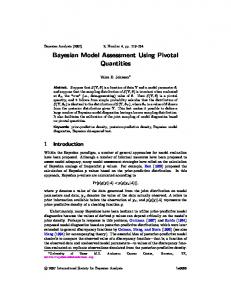
where e1 and e2 are independent Gaussian noise variables of standard deviation 0.05. As training data sets, we used the data sets that were used, e.g., in (MacKay, 1992; Neal, 1996) 2 . There are three data sets each containing 200 input-target pairs which were randomly generated by picking x1 uniformly from the ranges [-1.932,-0.453] and [+0.453,+1.932], and x2 uniformly from the range [0.534,3.142]. In order to get more accurate estimates of the true future utility, we generated additional 10000 input-target pairs having the same distribution for x1 and x2 as above, but without noise added to y1 and y2 . The true future utilities were then estimated using this test data set and integrating analytically over the noise in y1 and y2 . We used 8 hidden unit MLP with 47 parameters and GP model with 4 parameters (for GP model, training samples could be considered as parameters too). In both cases, we used Normal (N ) residual model. One hundred samples were drawn from the full posterior. See the prior and MCMC specification details in Appendix. The effective number of parameters was estimated to be about 30 for MLPs and about 50 for GP models. Figure 1 shows results from the MacKay’s Robot Arm problem where the utility is root mean square error. ISLOO-CV and 10-fold-CV give quite similar error estimates. Figure 2 shows that the importance sampling works probably very well for GP but it might produce wrong results for MLP. Although importance sampling weights for MLP are not very good, IS-LOO-CV results are not much different from the 10-fold-CV results in this simple problem. Note that as the uncertainty from not knowing the noise variance dominates (see below) small location errors or even large underestimation of the variance in the IS-LOO-CV predictive densities can not be seen in the estimates of the expected utilities. In Figure 1 realized, estimated and theoretical noise in each data set is also shown. Note that the estimated error is lower if the realized noise is lower and the uncertainty in estimated errors is about the same size as the uncertainty in the noise estimates. This demonstrates that most of the uncertainty in the estimate of the expected utility comes from not knowing the true noise variance. Figure 3 verifies this, as it shows the different components of the uncertainty in estimate of the expected utility. The variation from having slightly different training sets in 10-fold-CV and the variation from the Monte Carlo approximation are negligible compared to the variation from not knowing the true noise variance. The estimate of the variation from having slightly different training sets in 10-fold-CV was computed using the knowledge of the true function. In real world cases where the true function is unknown, this variation could be approximated using the CV terms calculated for bias correction, although this estimate might be too optimistic. Estimate of the variation from Monte Carlo approximation was computed directly 1 http://www.cs.toronto.edu/~radford/fbm.software.html 2 Available from http://wol.ra.phy.cam.ac.uk/mackay/Bayes_FAQ.html

On Bayesian Model Assesment and Choice Using Cross-Validation Predictive Densities

13

Realised noise in data Estimated noise (90% CI) Expected utility from posterior / Train error True future utility / Test error Expected utility with IS−LOO−CV (90% CI) Expected utility with 10−fold−CV (90% CI) MLP − Data 1

GP − Data 1

MLP − Data 2

GP − Data 2

MLP − Data 3

GP − Data 3

0.044

0.046 0.048 0.050 0.052 0.054 0.056 Standard deviation of noise / Root mean square error

0.058

Figure 1: Robot arm example: The expected utilities (root mean square errors) for MLPs and GPs. Results are shown for three different realizations of the data. IS-LOO-CV and 10-fold-CV give quite similar error estimates. Realized noise and estimated noise in each data set is also shown. Dotted vertical line shows the level of the theoretical noise. Note that the estimated error is lower if the realized noise is lower and the uncertainty in estimated errors is about the same size as the uncertainty in the noise estimates.

w (i) j

MLP − Data 1

Σ kj=1

Σ kj=1 Cum. weight

1

Cum. weight

w (i) j

On Bayesian Model Assesment and Choice Using Cross-Validation Predictive Densities

0.5

0

50 k MLP − Data 1

100

100

0

0

50 k GP − Data 1

100

100 150 Data point i

200

100

50

0

GP − Data 1 1

0.5

(i) Eff. sample size meff

(i) Eff. sample size meff

0

14

0

50

100 150 Data point i

200

50

0

0

50

Figure 2: Robot arm example: Two plot types were used to visualize the reliability of the importance sampling. Top plots show the total cumulative mass assigned to the k largest importance weights versus k (one line for each data point i). MLP has more mass attached to fewer weights. Bottom plots show the effective sample size of the importance sampling m ieff for each data point i (sorted in increasing order). The MLP has less effective samples. These two plots show that in this problem, IS-LOO-CV may be unreliable for the MLP, but probably works well for the GP.

from the Monte Carlo samples using the Bayesian bootstrap. Note that by estimating the ratio of the variance of the Monte Carlo approximation to full variance it is possible to check if using more Monte Carlo samples would improve accuracy. Figure 3 also shows that bias in 10-fold-CV, caused by the cross-validation predictive densities being based on slightly smaller data sets than full data set, is quite small. As the true function was known, we also computed estimate for the bias using the test data. For GP, the bias correction and the “true” bias were the same with about 2% accuracy. For MLP there was much more variance, but still all the “true” biases were inside the 90% confidence interval of the bias correction estimate. Although in this example, there would be no significant difference in reporting the expected utility estimates without the bias correction, bias may be significant in other problems. Especially, if there is reason to believe that the learning curve might be steep or if in model comparison two models might have different steepnes of the learning curves, it is advisable to compute the bias correction. In examples of sections subsection 3.3 and subsection 3.4 the bias correction had slight but more notable effect. Figure 4 demonstrates the difficulty of estimating the extrapolation capability of the model. As the distribution of the future data is estimated with the training data, it is not possible to know how well the model would predict outside the training data. Consequently, in model comparison we might choose a model with worse extrapolation capability. If it is possible to affect the data collection, it is advisable to be make sure that enough data is collected from the borders of assumed future data distribution, so that extrapolation for future predictions could be avoided. Figs. Figure 1 and Figure 6 demonstrate the comparison of models using paired comparison of the distributions of the expected utilities. Figure 1 shows the expected difference of root mean square errors and Figure 6 shows the expected ratio of mean predictive likelihoods (nth root of the pseudo-Bayes factors). IS-LOO-CV and 10-fold-CV give quite similar estimates, but disagreement shows slightly more clearly here when comparing models than when estimating expected utilities (compare to Figure 1). Disagreement between IS-LOO-CV and 10-fold-CV might be caused by bad importance weights of IS-LOO-CV for the MLPs (see Figure 2). Figure 7 shows different components of uncertainty in paired comparison of the distributions of the expected utilities. The variation from having slightly different training sets in 10-fold-CV and the variation from the Monte Carlo approximation have larger effect in pairwise comparison, but they are almost negligible compared to the

On Bayesian Model Assesment and Choice Using Cross-Validation Predictive Densities

15

10−fold CV (90% CI) Bias due to 10−fold CV using smaller training sets Variability due to having different training sets Variability due to Monte Carlo approximation MLP − Data 1

GP − Data 1

0.050

0.052

0.054 0.056 Root mean square error

0.058

Figure 3: Robot arm example: The components of the uncertainty and bias correction for the expected utility (root mean square errors) for MLP and GP. Results are shown for the data set 1. The variation from having slightly different training sets in 10-fold-CV and the variation from the Monte Carlo approximation are negligible compared to the variation from not knowing the true noise variance. The bias correction is quite small too, as it is about 0.6% of the mean error and about 6% of the 90% confidence interval of error.

Input points of data 3 Hull of the input points Full range of input

x2

3.0 2.5 2.0 1.5 1.0 0.5 −2.0

−1.5

−1.0

−0.5

0.0 x1

0.5

1.0

1.5

2.0

True future utility / Test error True future utility / Test error inside the hull True future utility / Test error outside the hull Expected utility with IS−LOO−CV (90% CI) Expected utility with 10−fold−CV (90% CI) MLP − Data 3

GP − Data 3 0.046

0.048

0.050 0.052 Root mean square error

0.054

0.056

Figure 4: Robot arm example: Upper plot shows input points of data set 3, with the full range (broken line) and with the realized range approximated by two convex hulls (solid line). Lower plot shows how the true future utility (test error) inside the hull coincides better with confidence interval for estimated expected utility.

On Bayesian Model Assesment and Choice Using Cross-Validation Predictive Densities

16

Expected utility from posterior / Train error True future utility / Test error Expected utility with IS−LOO−CV (90% CI) Expected utility with 10−fold−CV (90% CI)

MLP vs. GP − Data 1

MLP vs. GP − Data 2

MLP vs. GP − Data 3 ← MLP better −0.001

GP better →

0.000 0.001 Difference in root mean square errors

0.002

Figure 5: Robot arm example: The expected difference of root mean square errors for MLP vs. GP. Results are shown for three different realizations of the data. Disagreement between IS-LOO-CV and 10-fold-CV shows slightly more clearly when comparing models than when estimating expected utilities (compare to Figure 1). Figure 2 shows reason to suspect the reliability of IS-LOO-CV.

Expected utility with IS−LOO−CV (90% CI) Expected utility with 10−fold−CV (90% CI) MLP vs. GP − Data 1

MLP vs. GP − Data 2

MLP vs. GP − Data 3 ← GP better 0.94

MLP better → 0.96

0.98

1.00

1.02

1.04

Ratio of mean predictive likelihoods / PsBF1/n

Figure 6: Robot arm example: Expected ratio of mean predictive likelihoods (nth root of the pseudo-Bayes Factors) for MLP vs. GP. Results are shown for three different realizations of the data. Disagreement between IS-LOO-CV and 10-fold-CV shows slightly more clearly when comparing models than when estimating expected utilities (compare to Figure 1). Figure 2 shows reason to suspect the reliability of IS-LOO-CV.

On Bayesian Model Assesment and Choice Using Cross-Validation Predictive Densities

17

10−fold CV (90% CI) Bias due to 10−fold CV using smaller training sets Variability due to having different training sets Variability due to Monte Carlo approximation

MLP vs. GP − Data 1

0.000 0.001 Difference in root mean square errors

0.002

Figure 7: Robot arm example: The components of the uncertainty and bias correction for the expected difference of the expected root mean square errors for MLP vs. GP. Results are shown for the data set 1. The variation from having slightly different training sets in 10-fold-CV and the variation from the Monte Carlo approximation are almost negligible compared to the variation from not knowing the true noise variance. The bias correction is negligible in this case.

variation from not knowing the true noise variance. Figure 7 also shows that the bias in 10-fold-CV, caused by the cross-validation predictive densities being based on slightly smaller data sets than full data set, is quite small.

3.3

Real world problem I: Concrete quality estimation

In this section we present results from a real world problem of predicting the quality properties of concrete. The goal of the project was to develop a model for predicting the quality properties of concrete, as a part of a large quality control program of the industrial partner of the project. The quality variables included, e.g., compression strengths and densities for 1, 28 and 91 days after casting, and bleeding (water extraction), spread, slump and air%, that measure the properties of fresh concrete. These quality measurements depend on the properties of the stone material (natural or crushed, size and shape distributions of the grains, mineralogical composition), additives, and the amount of cement and water. In the study, we had 27 explanatory variables and 215 samples designed to cover the practical range of the variables, collected by the concrete manufacturing company. See the details of problem and the conclusions made by the concrete expert in (Järvenpää, 2001). It was very important to be able to describe the quality of the model in terms of the concrete expert instead of statistical jargon. It was also important to give good estimates of how reliable we believe our estimates were. We used MLP networks containing 10 hidden units with 322–335 parameters depending on the residual model and GP models with 30–258 parameters (note that heteroskedastic residual model used in GP requires one parameter for each data point). The residual models tested were Normal (N ), Student’s tν , input dependent Normal (in.dep.-N ) and input dependent tν . The Normal model was used as standard reference model. Student’s tν with unknown degrees of freedom ν was used as longer tailed robust residual model that allows small portion of samples to have large errors. When analyzing results from these two first residual models, it was noticed that the size of the residual variance varied considerably depending on three inputs, which were zero/one variables indicating the use of additives. In the input dependent residual models, the parameters of the Normal or Student’s tν were made dependent on these three inputs with common hyperprior. One hundred samples were drawn from the full posterior. See the prior and the MCMC specification details in Appendix. The effective number of parameters were estimated to be about 75–90 for MLPs (depending on the residual model) and about 80–100 for GP models. In the following, we report the results for one variable, air-%, which measures the volume percentage of air

On Bayesian Model Assesment and Choice Using Cross-Validation Predictive Densities

18

Expected utility with IS−LOO−CV (90% CI) Expected utility with 10−fold−CV (90% CI) MLP − N

GP − N 0.12

0.14 0.16 0.18 0.20 0.22 Normalized root mean square error

0.24

0.26

Expected utility with IS−LOO−CV (90% CI) Expected utility with 10−fold−CV (90% CI) MLP − N

GP − N 0.3

0.4

0.5 0.6 0.7 90%−quantile of absolute error

0.8

Figure 8: Concrete quality estimation example: The expected utilities for MLP and GP with the Normal (N ) residual model. Top plot shows the expected normalized root mean square errors and bottom plot shows the expected 90%-quantiles of absolute errors. IS-LOO-CV gives much lower estimates for MLP and somewhat lower estimates for GP than 10-fold-CV. Figure 9 shows reason to distrust IS-LOO-CV.

MLP − N

GP − N 100

(i) Effective sample size meff

(i) Effective sample size meff

100 75 50 25 0

0

50

100 150 Data point i

200

75 50 25 0

0

50

100 150 Data point i

200

Figure 9: Concrete quality estimation example: The effective sample sizes of the importance sampling m (i) eff for each data point

i (sorted in increasing order) for MLP and GP with the Normal (N ) noise model. Both models have many data points with small effective sample size which implies that IS-LOO-CV cannot be trusted.

in the concrete. As the air-% is positive and has a very skewed distribution (with mean 2.4% and median 1.7%) we used logarithmic transformation for the variable. This ensures the positiveness and allows use of much simpler additive residual models than in the case of nearly exponentially distributed variable. Figure 8 shows the expected normalized root mean square errors and the expected 90%-quantiles of absolute errors for MLP and GP with Normal (N ) residual model. The root mean square error was selected as general discrepancy utility and the 90%-quantile of absolute error was chosen after discussion with the concrete expert, who preferred this utility as easily understandable. IS-LOO-CV gives much lower estimates for MLP and somewhat lower estimates for GP than 10-fold-CV. Figure 9 shows that IS-LOO-CV for both MLP and GP has many data points with small (or very small) effective sample size. IS-LOO-CV cannot be used in this problem and although IS-LOO-CV results were computed for further models, those results are not shown here.

On Bayesian Model Assesment and Choice Using Cross-Validation Predictive Densities

19

Expected utility with 10−fold−CV (90% CI) GP − N GP − tν GP − in.dep.− N GP − in.dep.− tν 0.16

0.18 0.20 0.22 Normalized root mean square error

0.24

Expected utility with 10−fold−CV (90% CI) GP − N GP − tν GP − in.dep.− N GP − in.dep.− tν 0.40

0.45

0.50 0.55 0.60 90%−quantile of absolute error

0.65

Expected utility with 10−fold−CV (90% CI) GP − N GP − tν GP − in.dep.− N GP − in.dep.− tν 0.8

0.9 1.0 Mean predictive likelihood

1.1

Figure 10: The expected utilities for GP models with Normal (N ), Student’s tν , input dependent Normal (in.dep.-N ) and input dependent tν residual models. Top plot shows the expected normalized root mean square errors (smaller value is better), middle plot shows the expected 90%-quantiles of absolute errors (smaller value is better) and bottom plot shows the expected mean predictive likelihoods (larger value is better). Note that which residual model is favored and how much, depends on which utility is used. There is not much difference in expected utilities of different residual models if root mean square error is used as utility (it is easy to guess mean of prediction), but there is bigger differences if mean predictive likelihood is used instead (it is harder to guess distribution of the guess). See Tables 1, 2, and 3 for the pairwise comparisons of the residual models.

Figure 10 shows the expected normalized root mean square errors, the expected 90%-quantiles of absolute errors and the expected mean predictive likelihoods for GP models with Normal (N ), Student’s tν , input dependent Normal (in.dep.-N ) and input dependent tν residual models. Same results were computed also for MLPs and for example with input dependent tν noise, model difference between MLP and GP was quite small, but results are not shown here. Note that which residual model is favored and how much, depends on which utility is used. There is not much difference in expected utilities if root mean square error is used (it is easy to guess mean of prediction), but there is bigger differences if mean predictive likelihood is used instead (it is harder to guess the whole distribution of the guess). Tables 1, 2, and 3 show the results for the pairwise comparisons of the residual models. In this case, the uncertainties in comparison of the normalized root mean square errors and the 90%-quantiles of absolute errors are so big that no clear difference can be made between the models. As we get similar performance with all models (measured with these utilities), we could choose anyone of them without fear of choosing bad model (again measured with these utilities). With the mean predictive likelihood utility, there is more difference and by combining results from all three utilities and other preferences, we tipped to choose input dependent tν model.

On Bayesian Model Assesment and Choice Using Cross-Validation Predictive Densities

20

Table 1: Concrete quality estimation example: Pairwise comparison of GP models with different residual models using the normalized root mean square error as utility (see also Figure 10). The values in the matrix are probabilities that the method in the row is better than the method in the column. Uncertainties in the predictive utilities are so big (see also Figure 10) that no clear difference can be made between the residual models using the normalized root mean square error as utility.

residual model 1. N 2. tν 3. input dependent N 4. input dependent tν

1. 0.60 0.78 0.67

Comparison 2. 3. 0.40 0.22 0.18 0.82 0.69 0.15

4. 0.33 0.31 0.85

Table 2: Concrete quality estimation example: Pairwise comparison of GP models with different residual models using the 90%-quantile of absolute error as utility (see also Figure 10). The values in the matrix are probabilities that the method in the row is better than the method in the column. Uncertainties in the predictive utilities are so big (see also Figure 10) that no clear difference can be made between residual models using the 90%-quantile of absolute error as utility.

residual model 1. N 2. tν 3. input dependent N 4. input dependent tν

1. 0.83 0.47 0.79

Comparison 2. 3. 0.17 0.53 0.87 0.13 0.33 0.77

4. 0.21 0.67 0.23

Table 3: Concrete quality estimation example: Pairwise comparison of GP models with different residual models using mean predictive likelihood as utility (see also Figure 10). The values in the matrix are probabilities that the method in the row is better than the method in the column. It seems quite probable that the input dependent tν residual model is better than N or tν and is not much better than input dependent N .

Residual model 1. N 2. tν 3. input dependent N 4. input dependent tν

1. 0.98 0.99 1.00

Comparison 2. 3. 0.02 0.01 0.22 0.78 0.94 0.68

4. 0.00 0.06 0.32

On Bayesian Model Assesment and Choice Using Cross-Validation Predictive Densities

21

GP − Input dependent tν Expected utility with 10−fold−CV (90% CI) Samples with no additives Samples with additive A Samples with additive B All samples 0.2

0.3 0.4 0.5 0.6 0.7 0.8 90%−quantile of absolute error

0.9

Figure 11: Concrete quality estimation example: The expected utilities depending on the additives used for GP with the input dependent tν residual model. Knowing that additives have strong influence to the quality of concrete, it was useful to report also the expected utility separately for the samples with different additives. Plot shows the expected 90%-quantiles of absolute errors for samples with no additives, with additive A or B, and all samples.

It is also possible to compute the expected utilities assuming that future data distribution is different from the training data distribution. Knowing that additives have strong influence to the quality of concrete, it was useful to report also the expected utilities separately for samples with different additives (i.e., assuming that in all future casts no additives or just one of the additives will be used). Figure 11 shows for GP with input dependent tν residual model the expected 90%-quantiles of absolute errors for samples with no additives, with additive A or B, and all samples. Above we have presented the results for only one variable in the study. Rather similar results were obtained for the other variables.

3.4

Real world problem II: Forest scene classification

In this section, we demonstrate that if, due to dependencies in the data, several data points should be left out at a time, k-fold-CV has to be used to get reasonable results. The case problem is the classification of forest scenes with MLP (Vehtari et al., 1998). The final objective of the project was to assess the accuracy of estimating the volumes of growing trees from digital images. To locate the tree trunks and to initialize the fitting of the trunk contour model, a classification of the image pixels to tree and non-tree classes was necessary. We extracted a total of 84 potentially useful features: 48 Gabor filters (with different orientations and frequencies) that are generic features related to shape and texture, and 36 common statistical features (mean, variance and skewness with different window sizes). Fortyeight images were collected by using an ordinary digital camera in varying weather conditions. The labeling of the image data was done by hand via identifying many types of tree and background image blocks with different textures and lighting conditions. In this study, only pines were considered. We used 20 hidden unit MLP with 1808 parameters for 84 input model and 422 parameters for reduced 18 input model. Reduced input set was selected using Reversible Jump MCMC (RJMCMC) method (Green, 1995). Specific RJMCMC approach used for MLP input selection will be reported elsewhere. Likelihood model used was logistic. One hundred samples were drawn from the full posterior. See the prior and the MCMC specification details in Appendix. The effective number of parameters was estimated to be about 320 for 84 input model and 220 for 18 input model.

On Bayesian Model Assesment and Choice Using Cross-Validation Predictive Densities

22

(i) Effective sample size meff

100 Leave one point out at a time Leave one image out at a time 75

50

25

0

800

1600

2400 Data point i

3200

4000

4800

Figure 12: Forest scene classification example: The effective sample sizes of the importance sampling m (i) eff for each data point

i (sorted in increasing order) for 84 input logistic MLP. The effective sample sizes are calculated both for leave-one-point-out (IS-LOO-CV) and leave-one-image-out (IS-LOIO-CV). As data points from one image are dependent, cross-validation should be done by leaving one (or many) image(s) out at a time, but then posterior distribution changes too much to get reasonable importance weights. In this case, neither IS-LOO-CV nor IS-LOIO-CV can be trusted.

Textures and lighting conditions are more similar in different parts of one image than in different images. If the LOO-CV is used or data points are divided randomly in k-fold-CV, training and test sets (may) have data points from the same image, which would lead to too optimistic estimates of predictive utility. In order to get realistic estimate of the predictive utility for new unseen images, training data set has to be divided by images. As seen in section subsection 3.3 leaving one point out can change posterior so much that importance sampling does not work. Leaving one image (100 data points) out will change posterior even more. Figure 12 shows the effective sample sizes of the importance sampling for 84 input MLP for IS-LOO-CV and IS-LOIO-CV (leave-oneimage-out) (for the 18 input model, the plot was similar). The expected classification errors for 84 and 18 input MLPs are shown in Figure 13. The predictive utility computed from the posterior predictive distribution (train error) gives too low estimates. IS-LOO-CV and 8-foldCV with random data division give too low estimates because data points from one image are dependent. ISLOO-CV also suffers from somewhat bad importance weights and IS-LOIO-CV suffers from very bad importance weights (see also Figure 12). In group 8-fold-CV, the data divison was made by handling all the data points from one image as one nondividable group. As there was 48 images, six images were left out at a time. Pairwise comparison computed from group 8-fold-cv predictive distributions gives probability 0.86 that 84 input model has lower expected classification error than 18 input model. We might still use the smaller model for classification, as it would be not much worse, but slightly faster.

4 Conclusions We have discussed the problem of estimating the distribution of the expected utility of the Bayesian model using the cross-validation predictive densities. The IS-LOO-CV predictive densities are a quick way to estimate the expected utilities and the approach can be used in some cases with flexible non-linear models such as MLP and GP. If diagnostics hint that importance weights are not good, we can instead use the k-fold-CV predictive densities with the bias correction. Using k-fold-CV takes k times more time, but it is more reliable. In addition, if data points have certain dependencies, k-fold-CV has to be used to get reasonable results. We proposed a quick and generic approach based on the Bayesian bootstrap for obtaining samples from the distributions of the expected utilities.

On Bayesian Model Assesment and Choice Using Cross-Validation Predictive Densities

23

Expected utility from posterior / Train error Expected utility with IS−LOO−CV (90% CI) Expected utility with IS−LOIO−CV (90% CI) Expected utility with random 8−fold−CV (90% CI) Expected utility with group 8−fold−CV (90% CI) MLP − 84 inputs

MLP − 18 inputs

4

6

8 10 Classification error %

12

14

Figure 13: Forest scene classification example: The expected utilities (classification errors) for 84 and 18 input logistic MLPs. IS-LOO-CV gives too low estimate because data points from one image are dependent (and also because of somewhat bad importance weights) and IS-LOIO-CV gives too low estimate because of bad importance weights when leaving one image out at time (see Figure 12). 8-fold-cv with random data division gives too low estimate because data points from one image are dependent. In group 8-fold-CV, the data divison was made by handling all the data points from one image as one nondividable group.

With the proposed method, it is easy to compute the probability that one method has better expected utility than another one.

Acknowledgments This study was partly funded by TEKES Grant 40888/97 (Project PROMISE, Applications of Probabilistic Modeling and Search) and Graduate School in Electronics, Telecommunications and Automation (GETA). The authors would like to thank Dr. H. Järvenpää for providing her expertise into the concrete case study.

Bibliography Aitkin, M. (1991). Posterior Bayes factors (with discussion). Journal of the Royal Statistical Society B, 53(1):111–142. Berger, J. and Pericchi, L. (1996). The intrinsic Bayes factor for model selection and prediction. Journal of the American Statistical Association, 91(433):109–122. Bernardo, J. M. and Smith, A. F. M. (1994). Bayesian Theory. John Wiley & Sons. Breiman, L., Friedman, J., Olshen, R., and Stone, C. (1984). Classification and regression trees. Chapman and Hall. Burman, P. (1989). A comparative study of ordinary cross-validation, v-fold cross-validation and the repeated learning-testing methods. Biometrika, 76(3):503–514.

On Bayesian Model Assesment and Choice Using Cross-Validation Predictive Densities

24

Burman, P., Chow, E., and Nolan, D. (1994). A cross-validatory method for dependent data. Biometrika, 81(2):351–358. Carlin, B. P. and Chib, S. (1995). Bayesian model choice via Markov chain Monte Carlo methods. Journal of the Royal Statistical Society B, 57(3):473–484. Dietterich, T. G. (1998). Approximate statistical tests for comparing supervised classification learning algorithms. Neural Computation, 10(7):1895–1924. Duane, S., Kennedy, A. D., Pendleton, B. J., and Roweth, D. (1987). Hybrid Monte Carlo. Physics Letters B, 195(2):216–222. Geisser, S. (1975). The predictive sample reuse method with applications. Journal of the American Statistical Association, 70(350):320–328. Geisser, S. and Eddy, W. F. (1979). A predictive approach to model selection. Journal of the American Statistical Association, 74(365):153–160. Gelfand, A. E. (1996). Model determination using sampling-based methods. In Gilks, W. R., Richardson, S., and Spiegelhalter, D. J., editors, Markov Chain Monte Carlo in Practice, pages 145–162. Chapman & Hall. Gelfand, A. E. and Dey, D. K. (1994). Bayesian model choice: asymptotics and exact calculations. Journal of the Royal Statistical Society B, 56(3):501–514. Gelfand, A. E., Dey, D. K., and Chang, H. (1992). Model determination using predictive distributions with implementation via sampling-based methods (with discussion). In Bernardo, J. M., Berger, J. O., Dawid, A. P., and Smith, A. F. M., editors, Bayesian Statistics 4, pages 147–167. Oxford University Press. Gelman, A. (1996). Inference and monitoring convergence. In Gilks, W. R., Richardson, S., and Spiegelhalter, D. J., editors, Markov Chain Monte Carlo in Practice, pages 131–144. Chapman & Hall. Gelman, A., Carlin, J. B., Stern, H. S., and Rubin, D. R. (1995). Bayesian Data Analysis. Chapman & Hall. Geman, S. and Geman, D. (1984). Stochastic relaxation, Gibbs distributions and the Bayesian restoration of images. IEEE Transactions on Pattern Analysis and Machine Intelligence, 6(2):721–741. Geweke, J. (1989). Bayesian inference in econometric models using Monte Carlo integration. Econometrica, 57(6):1317–1339. Geweke, J. (1993). Bayesian treatment of the independent Student-t linear model. Journal of Applied Econometrics, 8(Supplement):S19–S40. Gilks, W. R. (1995). Discussion: Fractional Bayes factors for model comparison. Journal of the Royal Statistical Society B, 57(1):119. Green, P. (1995). Reversible jump Markov chain Monte Carlo computation and Bayesian model determination. Biometrika, 82:711–732. Järvenpää, H. (2001). Quality characteristics of fine aggregates and controlling their effects on concrete. PhD thesis, Helsinki University of Technology. Kass, R. E. and Raftery, A. E. (1995). 90(430):773–795.

Bayes factors.

Journal of the American Statistical Association,

Künsch, H. R. (1989). The jackknife and the bootstrap for general stationary observations. Annals of Statistics, 17(3):1217–1241. Künsch, H. R. (1994). Discussion: Approximate Bayesian inference with the weighted likelihood bootstrap. Journal of the Royal Statistical Society B, 56(1):39.

On Bayesian Model Assesment and Choice Using Cross-Validation Predictive Densities

25

Kong, A., Liu, J. S., and Wong, W. H. (1994). Sequential imputations and Bayesian missing data problems. Journal of the American Statistical Association, 89(425):278–288. Lampinen, J. and Vehtari, A. (2001). Bayesian approach for neural networks – review and case studies. Neural Networks, 14(3):7–24. Liu, J. S. and Chen, R. (1995). Blind deconvolution via sequential imputations. Journal of the American Statistical Association, 90(430):567–576. Lo, A. Y. (1987). A large sample study of the Bayesian bootstrap. Annals of Statistics, 15(1):360–375. MacEachern, S. N. and Peruggia, M. (2000). Importance link function estimation for Markov chain Monte Carlo methods. Journal of Computational and Graphical Statistics, 9(1):99–121. MacKay, D. J. C. (1992). A practical Bayesian framework for backpropagation networks. Neural Computation, 4(3):448–472. MacKay, D. J. C. (1998). Introduction to Monte Carlo methods. In Jordan, M. I., editor, Learning in Graphical Models. Kluwer Academic Publishers. Mason, D. M. and Newton, M. A. (1992). A rank statistics approach to the consistency of a general bootstrap. Annals of Statistics, 20(3):1611–1624. Müller, P. and Rios Insua, D. (1998). Issues in Bayesian analysis of neural network models. Neural Computation, 10(3):571–592. Nadeau, C. and Bengio, Y. (1999). Inference for the generalization error. Technical Report 99s-25, CIRANO, Montreal. Neal, R. M. (1996). Bayesian Learning for Neural Networks. Springer-Verlag. Neal, R. M. (1997). Monte Carlo implementation of Gaussian process models for Bayesian regression and classification. Technical Report 9702, Dept. of Statistics, University of Toronto. Neal, R. M. (1998). Assessing relevance determination methods using DELVE. In Bishop, C. M., editor, Neural Networks and Machine Learning, pages 97–129. Springer-Verlag. Neal, R. M. (1999). Regression and classification using Gaussian process priors (with discussion). In Bernardo, J. M., Berger, J. O., Dawid, A. P., and Smith, A. F. M., editors, Bayesian Statistics 6, pages 475–501. Oxford University Press. Neal, R. M. (2000). Software for Flexible Bayesian Modeling [online]. Release 2000-08-21. Available at: http://www.cs.toronto.edu/~radford/fbm.software.html. Newton, M. A. and Raftery, A. E. (1994). Approximate Bayesian inference with the weighted likelihood bootstrap (with discussion). Journal of the Royal Statistical Society B, 56(1):3–48. O’Hagan, A. (1995). Fractional Bayes factors for model comparison (with discussion). Journal of the Royal Statistical Society B, 57(1):99–138. Peruggia, M. (1997). On the variability of case-deletion importance sampling weights in the Bayesian linear model. Journal of the American Statistical Association, 92(437):199–207. Pinto, R. L. and Neal, R. M. (2001). Improving Markov chain Monte Carlo estimators by coupling to an approximating chain. Technical Report 0101, Dept. of Statistics, University of Toronto. Rasmussen, C. E. and Højen-Sørensen, P. A. (2000). Empirical model comparison: Bayesian analysis of disjoint cross validation for continuous losses [online]. Extended abstract for NIPS*2000 Workshop on Cross-Validation, Bootstrap and Model Selection, Available at: http://www.cs.cmu.edu/~rahuls/nips2000/Abstracts/Rasmussen.ps.gz.

On Bayesian Model Assesment and Choice Using Cross-Validation Predictive Densities

26

Rasmussen, C. E., Neal, R. M., Hinton, G. E., van Camp, D., Revow, M., Ghahramani, Z., Kustra, R., and Tibshirani, R. (1996). The DELVE manual [online]. Version 1.1. Available at: ftp://ftp.cs.utoronto.ca/pub/neuron/delve/doc/manual.ps.gz. Robert, C. P. and Casella, G. (1999). Monte Carlo Statistical Methods. Springer-Verlag. Rubin, D. B. (1981). The Bayesian bootstrap. Annals of Statistics, 9(1):130–134. Shao, J. (1993). Linear model selection by cross-validation. Journal of the American Statistical Association, 88(422):486–494. Spiegelhalter, D. J., Best, N. G., and Carlin, B. P. (1998). Bayesian deviance, the effective number of parameters, and the comparison of arbitrarily complex models. Technical Report 98-009, Division of Biostatistics, University of Minnesota. Stephens, M. (2000). Bayesian analysis of mixtures with an unknown number of components — an alternative to reversible jump methods. Annals of Statistics, 28(1):40–74. Stone, M. (1974). Cross-validatory choice and assessment of statistical predictions (with discussion). Journal of the Royal Statistical Society B, 36(2):111–147. Sundararajan, S. and Keerthi, S. S. (2000). Predictive ing hyperparameters in Gaussian processes [online]. http://guppy.mpe.nus.edu.sg/~mpessk/gp/gp_nc.ps.gz.

approaches for choosPreprint. Available at

Vehtari, A., Heikkonen, J., Lampinen, J., and Juujärvi, J. (1998). Using Bayesian neural networks to classify forest scenes. In Casasent, D. P., editor, Intelligent Robots and Computer Vision XVII: Algorithms, Techniques, and Active Vision, pages 66–73. SPIE. Vehtari, A., Särkkä, S., and Lampinen, J. (2000). On MCMC sampling in Bayesian MLP neural networks. In Amari, S.-I., Giles, C. L., Gori, M., and Piuri, V., editors, IJCNN’2000: Proceedings of the 2000 International Joint Conference on Neural Networks, volume I, pages 317–322. IEEE. Weng, C.-S. (1989). On a second-order asymptotic property of the Bayesian bootstrap mean. Annals of Statistics, 17(2):705–710.

Appendix: Prior and MCMC specification details Short description of the prior and the MCMC specification details is given here. See (Neal, 1996, 1997, 1999; Lampinen and Vehtari, 2001) and the FBM software manual (Neal, 2000) for additional details. The MCMC sampling was done with the FBM 3 software and Matlab-code derived from the Netlab4 toolbox. FBM was used when possible (normal and logistic models) because of its speed. Matlab-based implementation was slower, but it was much easier to implement new features to it. In the following, we use the notation r ∼ F(a) as shorthand for p(r ) = F(r |a) where a denotes the parameters of the distribution F, and the random variable argument r is not shown explicitly. N (µ, σ 2 ) denotes a normal distribution with mean µ and variance σ 2 . Parametrization of the Inverse Gamma here is   1 2 −2 2 2 2 −(ν/2+1) , Inv-gamma(σ |σ0 , ν) ∝ (σ ) exp − νσ0 σ 2 3 http://www.cs.toronto.edu/~radford/fbm.software.html 4 http://www.ncrg.aston.ac.uk/netlab/

On Bayesian Model Assesment and Choice Using Cross-Validation Predictive Densities

27

which is equal to a scaled inverse chi-square distribution (Gelman et al., 1995, Appendix A). The parameter ν is the number of degrees of freedom and σ02 is a scale parameter. We first describe common details for MLP and GP and then specific details for each case.

MLP We used one hidden layer MLP with tanh hidden units, which in matrix format can be written as

 f (x, θw ) = b2 + w 2 tanh b1 + w 1 x .

The θw denotes all the parameters w1 , b1 , w 2 , b2 , which are the hidden layer weights and biases, and the output layer weights and biases, respectively. The Gaussian priors for the weights were w 1 ∼ N (0, αw1 ) b1 ∼ N (0, αb1 ) w 2 ∼ N (0, αw2 ) b2 ∼ N (0, αb2 ) where the α’s are the variance hyperparameters. The conjugate inverse Gamma hyperprior for αj ’s is α j ∼ Inv-gamma(α0, j , να, j )

The fixed values for the highest level hyperparameters in the case studies were similar to those used in (Neal, 1996, 1998). The hyperpriors for w1 and w2 were scaled according to the number of inputs K and hidden units J . Typical values were να,w1 = 0.5 α0,w1 = (0.05/K

1/να,w1 2

) .

ARD prior was used for input weights w 1j,k ∼ N (0, αk,w1 ), αk,w1 ∼ Inv-gamma(α¯ w1 , να,w1 ) α¯ w1 ∼ Inv-gamma(α¯ 0,w1 , να,w ¯ 1 ), where the average scale of the αk is determined by the next level hyperparameters. Sampling of the weights was done with HMC and sampling of the hyperparameters was done with Gibbs sampling.

GP We used a simple covariance function producing smooth functions p

 ( j) 2 2 2 (i) Ci j = η exp − ρu (xu − xu ) + δi j J 2 + δi j σe2 . u=1

Jitter was fixed to

J2

= 0.01. Inverse Gamma prior for scale was η2 ∼ Inv-gamma(αη2 , νη2 )

And ARD prior was used for relevance parameters ρu2 ∼ Inv-gamma(αρ 2 , νρ 2 ) αρ 2 ∼ Inv-gamma(α0,ρ 2 , ν0,ρ 2 ), Sampling of the parameters was done with HMC.

On Bayesian Model Assesment and Choice Using Cross-Validation Predictive Densities

28

Robot Arm The Normal residual model with Inverse Gamma prior for variance was used e ∼ N (0, σ 2 ) σ 2 ∼ Inv-gamma(σ02 , νσ ). Prior specification for MLP model specified in FBM notation was net-spec log 2 8 2 / - x0.05:0.5:1 0.05:0.5 - x0.05:0.5 - 1 model-spec log real 0.05:0.5

1/ν

These commands set hyperparameters of parameter priors to values: να,w1 = 0.5, α¯ 0,w1 = (0.05/2 α,w1 )2 , 1/να,w2 2 2 να,w ) , αb2 = 1, and Normal residual ¯ 1 = 1, να,b1 = 0.5, α0,b1 = 0.05 , να,w2 = 0.5, α0,w2 = (0.05/8 model parameters to σ0 = 0.05, and νσ = 0.5. MCMC specification for MLP model in FBM notation was net-gen log fix 0.1 0.5 mc-spec log repeat 10 heatbath hybrid 10 0.05 net-mc log 1 mc-spec log repeat 50 sample-sigmas heatbath hybrid 10 0.15 net-mc log 2 mc-spec log repeat 50 sample-sigmas heatbath 0.9 hybrid 10 0.2 negate net-mc log 3 mc-spec log repeat 500 sample-sigmas heatbath 0.9 hybrid 10 0.4 negate net-mc log 1000

net-gen intializes weights to zero and following paramteres as αk,w1 = 0.1, αb1 = 0.1, αw2 = 0.5, and σ = 0.1. First three mc-spec specifications are used to improve convergence and last mc-spec specification specifies the main run (net-mc does the sampling). The last mc-spec specification means: alternate Gibbs sampling and HMC with chain length 10, step size 0.4, and persistence 0.9, save every 500th iteration and last net-mc does iterations until 1000 iterations are saved. See FBM manual for full details. All samples were used to estimate convergence and autocorrelations. For predictive densities 100 samples were used (every ninth sample starting from sample 100). Prior specification for GP model specified in FBM notation gp-spec log 2 2 - - 0.01 / 0.05:0.5 0.05:0.5:1 model-spec log real 0.05:0.5

These commands set hyperparameters of parameter priors to values: J = 0.01, αη2 = 0.052 , νη2 = 0.5, νρ 2 = 0.5, α0,ρ 2 = 0.052 , ν0,ρ 2 = 1, and Normal residual model parameters to σ0 = 0.05, and νσ = 0.5. MCMC specification for GP model in FBM notation

gp-gen log fix 0.2 0.1 mc-spec log repeat 5 heatbath hybrid 10 0.1 gp-mc log 1 mc-spec log repeat 5 heatbath hybrid 10 0.4 sample-variances gp-mc log 1000

gp-gen intializes following paramteres as η2 = 0.2, ρu2 = 0.1 and σ = 0.2. First mc-spec specification is used to improve convergence (per-case variances are not yet sampled) and second mc-spec specification specifies the

On Bayesian Model Assesment and Choice Using Cross-Validation Predictive Densities

29

main run (gp-mc does the sampling). The last mc-spec specification means: aletranate HMC with chain length 10, step size 0.4, no persistence and sampling per-case variances with Gibbs sampling, save every 5th iteration and last gp-mc does iterations until 1000 iterations are saved. See the FBM manual for full details. All samples were used to estimate convergence and autocorrelations. For predictive densities 100 samples were used (every ninth sample starting from sample 100).

Concrete Quality Estimation Prior specifications for MLPs and GPs were same as in robot arm case except for parameters of alternative residual models. For MLP, we used Student’s t-distribution, where the tails can be controlled by choosing the number of degrees of freedom ν in the distribution. The integration over the degrees of freedom was done by Gibbs sampling for discretized values of ν, so that the residual model is e ∼ tν (0, σ 2 ) ν = V [i] i ∼ Ud (1, K ) V [1 : K ] = [2, 2.3, 2.6, 3, 3.5, 4, 4.5, 5 : 1 : 10, 12 : 2 : 20, 25 : 5 : 50] σ 2 ∼ Inv-gamma(σ0 , νσ ) where [a : s : b] denotes the set of values from a to b with step s, and Ud (a, b) is a uniform distribution of integer values between a and b. For GP instead of Student’s t-distribution, we used per-case residual variance model, with Inverse-Gamma prior having unknown degrees of freedom en ∼ N (0, (σ 2 )n ) (σ 2 )n ∼ Inv-gamma(σave , νσ ) νσ ∼ Inv-gamma(σν , νν ) σave ∼ Inv-gamma(σ0 , νσ,ave ), where the fixed hyperparameters are σν , νν , σ0 and νσ,ave . This is equal to the tν -distribution residual model with unknown degrees of freedom νσ (Geweke, 1993), but easier to implement for GP (Neal, 1999). We also used input dependent Normal and tnu residual models. Three inputs, which were zero/one variables indicating use of additives, divide the data to six groups. For each group, we had own residual model parameters with common hyperprior. For example for input dependent Normal model (in.dep.-N ) we had 2 ei ∼ N (0, σl(i) )

σl2 ∼ Inv-gamma(σ 2 , νσl ) σ 2 ∼ Inv-gamma(σ02 , νσ ), where l is index of group, and l(i) is index of group to which ith data point belongs. For MLP the main HMC parameters were: the length of individual chains was 100, step size 0.5 with Neal’s heuristic step size adjustment, persistence parameter 0.9, and window length in windowing 5. The burn-in stage contained 16 000 iterations and the actual sampling 80 000 iterations, from which 100 samples were stored for the analysis.

On Bayesian Model Assesment and Choice Using Cross-Validation Predictive Densities

30

For GP the main HMC parameters were: the length of individual chains was 100, step size 0.4 with Neal’s heuristic step size adjustment and persistence parameter 0.9. The burn-in stage contained 200 iterations and the actual sampling 1 000 iterations, from which 100 samples were stored for the analysis.

Forest scene classification 1/να,w1 2 )

Prior specifications for MLP was same as in robot arm case except α¯ 0,w1 = (0.2/2 mation was used to compute the probability that a binary-valued target, y, has value 1

and logistic transfor-

p(y = 1|x, θw , M) = [1 + exp(− f (x, θw ))]−1 . The main HMC parameters were: the length of individual chains was 10, step size 0.2 with Neal’s heuristic step size adjustment, persistence parameter 0.95. The burn-in stage contained 5000 iterations and the actual sampling 45 000 iterations, from which 100 samples were stored for the analysis.