erally, Bayes-UCB appears as an unifying framework for several variants of the
UCB algorithm addressing different bandit prob- lems (parametric multi-armed ...
On Bayesian Upper Confidence Bounds for Bandit Problems
Emilie Kaufmann
Olivier Capp´ e LTCI, CNRS & Telecom ParisTech
Abstract
In contrast, in the Bayesian approach each arm is characterized by a parameter which is endowed with a prior distribution. The Bayesian performance is then defined as the average performance over all possible problem instances weighted by the prior on the parameters. In this work, we argue that algorithms derived from the Bayesian perspective also prove efficient when evaluated using frequentist measures of performance. Before exposing our contributions more precisely, we start by reviewing some aspects of these two alternative views.
Stochastic bandit problems have been analyzed from two different perspectives: a frequentist view, where the parameter is a deterministic unknown quantity, and a Bayesian approach, where the parameter is drawn from a prior distribution. We show in this paper that methods derived from this second perspective prove optimal when evaluated using the frequentist cumulated regret as a measure of performance. We give a general formulation for a class of Bayesian index policies that rely on quantiles of the posterior distribution. For binary bandits, we prove that the corresponding algorithm, termed BayesUCB, satisfies finite-time regret bounds that imply its asymptotic optimality. More generally, Bayes-UCB appears as an unifying framework for several variants of the UCB algorithm addressing different bandit problems (parametric multi-armed bandits, Gaussian bandits with unknown mean and variance, linear bandits). But the generality of the Bayesian approach makes it possible to address more challenging models. In particular, we show how to handle linear bandits with sparsity constraints by resorting to Gibbs sampling.
1
Aur´ elien Garivier
In the classical parametric stochastic multi-armed bandit model, an agent faces K independent arms which depend on unknown parameters θ1 , . . . , θK ∈ Θ. The draw of arm j at time t results in a reward Xt that is extracted from the i.i.d sequence (Yj,t )t≥1 marginally distributed under νθj , whose expectation is denoted by µj . The agent sequentially draws the arms according to a strategy (It )t≥1 , where It denotes the arm chosen at round t, based on previous rewards Xs = Ys,Is for 1 ≤ s ≤ t − 1. The agent’s goal is to maximize Pnthe expected cumulated reward until time n, Eθ [ t=1 Xt ], or, equivalently, to minimize the cumulated regret " n # K X X ∗ Rn (θ) = Eθ µ − µIt = (µ∗ − µj )Eθ [Nn (j)] , t=1
j=1
(1) where µ∗ = max{µj : 1 ≤ j ≤ K} and Nn (j) denotes the number of draws of arm j up to time n.
Introduction
The literature on stochastic multi-armed bandit problems is separated in two distinct approaches. In the frequentist view, the expected mean rewards corresponding to all arms are considered as unknown deterministic quantities and the goal of the algorithm is to achieve the best parameter-dependent performance. Appearing in Proceedings of the 15th International Conference on Artificial Intelligence and Statistics (AISTATS) 2012, La Palma, Canary Islands. Volume XX of JMLR: W&CP XX. Copyright 2012 by the authors.
592
Lai & Robbins [12], followed by Burnetas & Katehakis [3], have provided lower bounds on the number of suboptimal draws under any good strategy (having o(n) regret for all bandit problems): for any arm j such that µj < µ∗ , lim inf n→∞
1 Eθ [Nn (j)] ≥ , (2) log(n) inf θ∈Θ:µ(θ)>µ∗ KL(νθj , νθ )
where KL denotes the Kullback-Leibler divergence. For important classes of distributions, recent contributions have provided finite-time analysis of strategies that are asymptotically optimal in so far that they reach this lower bound. Following [10], [5] and [15] have analyzed algorithms based on the celebrated
On Bayesian Upper Confidence Bounds for Bandit Problems
upper confidence bound (UCB) principle of [1] for, respectively, one-parameter exponential models and finitely-supported distributions. When considering the multi-armed bandit model from a Bayesian point of view, one assumes that the parameter θ = (θ1 , ..., θK ) is drawn from a prior distribution. More precisely, we will assume in the following that the parameters (θj )1≤j≤K are drawn independently from prior distributions (πj )1≤j≤K (usually chosen to be all equal), and that conditionally on (θj )1≤j≤K , the sequences (Y1,t )t≥1 , . . . , (YK,t )t≥1 are jointly independent and i.i.d. with marginal distributions νθ1 , . . . , νθK . In P this Bayesian setting, the goal is to maximize n E [ t=1 Xt ], where the expectation is relative to the entire probabilistic model, including the randomization over θ. Bayesian optimality can equivalently be measured considering the Bayesian regret RnB = E[Rn (θ)] that averages the regret over the parameters. A major appeal of the Bayesian framework is the fact that a strategy with minimal Bayesian regret can be described, if not always computed. To define the Bayesian strategy, let Πt denote the posterior distribution of θ after t rounds of game, with Π0 denoting the initial prior distribution. Due to our choice of independent priors on (θj )1≤j≤K , Πt is a product distribution which is equivalently defined by t . If at the marginal posterior distributions π1t , ..., πK round t one chooses arm It = j and consequently observes Xt = Yj,t , the Bayesian update for arm j is πjt (θj ) ∝ νθj (Xt ) πjt−1 (θj ) ,
(3)
whereas for i 6= j, πit = πit−1 . A Bayesian algorithm is allowed to exploit the knowledge of the whole posterior Πt to determine the next action It+1 . In his seminal paper [7], Gittins showed that, for models admitting sufficient statistics, finding the Bayesian optimal strategy is equivalent to solving the planning problem in a related Markov decision model. Moreover, for several important cases, including that of Bernoulli rewards with Beta priors, the planning problem can be solved numerically thanks to a clever problem reduction using so-called ’Gittins indices’. Gittins originally considered the infinite-horizon discounted P∞ problem in which one tries to maximize E [ t=1 γ t Xt ], where 0 < γ < 1 is a real discount parameter. It is possible to show that the model reduction argument still holds when the horizon is known, making it possible to compute a finite-horizon variant of Gittins indices and, thus, to determine the finite-horizon Bayesian optimal strategy. The details of the corresponding algorithm are omitted here because of space limitations and we refer to the recent 593
work of Ni˜ no-Mora [13] for discussion of the numerical complexity of this approach. However, we report in Section 4 some experiments on Bernoulli bandits that illustrate our finding that the corresponding policy constantly outperforms its frequentist UCB-like competitors on their own ground, that is, when evaluated using the parameter-dependent (frequentist) regret. Interestingly, Lai [11] established lower bounds for the Bayesian risk (depending on the prior) and showed (in particular cases) that algorithms reaching the lower-bound (2) were also Bayesian-optimal. Conversely, our finding that the Bayesian optimal strategy also achieves remarkable parameter-dependent performance for most (all?) value of the parameter θ is currently not supported by mathematical arguments. Furthermore, computing the finite-horizon variant of the Gittins indices is only feasible for moderate horizons due to the need to repeatedly perform (and store the results of) dynamic programming recursions on reduced models. Even for small horizons, the associated computational load and memory footprint are orders of magnitude larger than those of the UCB-like algorithms considered in [1, 10, 5, 15]. Our objective is thus to propose a generic bandit algorithm, termed Bayes-UCB, that is inspired by the Bayesian interpretation of the problem but retains the simplicity of UCB-like algorithms. Our hope is that this algorithm is simple enough to be effectively implemented and yet sufficiently close to the Bayesian optimal policy to be able to reach the asymptotic lower bound of (2), including in cases that are currently not handled by UCB-like algorithms. In addition to promising simulation results reported in Section 4, we provide several significant elements that support our hopes. First, it is shown in Section 2 that instantiating the generic Bayes-UCB algorithm in different specific cases (one-parameter exponential families rewards, Gaussian-armed bandit with unknown means and variances, linear bandits, Gaussian process optimization) yields algorithms that share striking similarities with methods previously proposed in the literature. In the case of Bernoulli rewards, we provide in Section 3 (with corresponding proofs in appendix) a complete finite-time analysis of the Bayes-UCB algorithm that implies that it reaches the lower bound of (2). The proof of this result also reveals some enlightening facts about the construction of upper confidence bounds used in recently proposed variants of UCB such as those of [2, 5]. Finally, in Section 4, we consider the challenging setting of sparse linear bandits where we show how the Bayes-UCB strategy, using a sparsity inducing prior, can be numerically approximated using Markov Chain Monte Carlo simulations.
Emilie Kaufmann, Olivier Capp´ e, Aur´ elien Garivier
2
The Bayes-UCB algorithm
We start by presenting the rationale for the proposed algorithm before stating it more formally. First, being inspired by the Bayesian modeling of the bandit problem, the Bayes-UCB strategy is a function of the posteriors (πjt )1≤j≤K . Due to the nature of our performance measure, the relevant aspect of θj is the expectation µj . Hence, denoting by λtj , for 1 ≤ j ≤ K, the posterior distribution of the mean µj induced by πjt , the proposed strategy is a function of (λtj )1≤j≤K only. A similar principle is used in the so-called Thompson strategy which consists in drawing samples from the distributions (λtj )1≤j≤K so as to select an arm j with probability equal to the posterior probability that its mean µj is the highest [18]. The Bayesian Learning Automaton advocated by [9] uses this idea of sampling the posterior, but no regret analysis is provided. The use of fixed-level quantiles of (λtj )1≤j≤K as confidence indices appears in [14] as a special case of the Interval Estimation method. To be more specific, denote by Q(t, ρ) the quantile function associated to the distribution ρ, such that Pρ (X ≤ Q(t, ρ)) = t. [14] use indices of the form Q(1 − α, λtj ) for 1 ≤ j ≤ K, with α chosen to be equal to a few percents. In BayesUCB, we acknowledge the strong similarity between these posterior indices based on quantiles and the upper confidence bounds used in UCB and its variants: we consider indices of the form Q(1 − αt , λtj ), where αt is of order 1/t. As will be shown in Section 3 below for the case of binary rewards, this 1/t rate is deeply connected with the form of the upper confidence bounds used in variants of UCB that are known to reach the bound in (2). It is conjectured that no other rate can provide an algorithm that reaches the bound in (2) and that, furthermore, choices of the form 1/tβ with β < 1 do not even guarantee a finite-time logarithmic control of the regret. As a more pragmatic comment, we also observed in experiments not reported here that, in the case of binary rewards, the empirical performance of the method were superior when using αt ≡ 1/t. We are now ready to state the generic version of the BayesUCB algorithm. In Algorithm 1, the horizon-dependent term (log n)c is an artefact of the theoretical analysis that enables us, for c ≥ 5, to both guarantee finite-time logarithmic regret bounds and achieve asymptotic optimality with respect to (2). But in simulations, the choice c = 0 actually proved to be the most satisfying. In cases where the prior Π0 is chosen to correspond to an improper prior (see, e.g., the Gaussian models below), qj (t) is not defined when t = 1. In those cases it suffices, as is commonly done in most bandit algorithms, to make sure that initially one gathers a sufficient number of observations to guarantee that the posterior Πt indeed 594
Algorithm 1 Bayes-UCB Require: n (horizon), Π0 (initial prior on θ) c (parameters of the quantile) 1: for t = 1 to n do 2: for each arm j = 1, . . . , K do 3: compute � � 1 t−1 , λ qj (t) = Q 1 − t(log n)c j end for draw arm It = arg maxj=1...K qj (t) get reward Xt = YIt ,t and update Πt according to (3) 7: end for 4: 5: 6:
becomes proper, for instance by drawing each arm a few times. As such, Algorithm 1 corresponds to a general principle that does not even require that the prior Π0 be chosen as a product distribution: in fact, the GP-UCB algorithm for gaussian processes [17] can be seen as a variant of Bayes-UCB in which dependencies, in contrast, are of fundamental importance; but this is not a point that we emphasize in this article, and for the simplicity of notation we focus on the case where the coordinates of θ are independent. Implementing Algorithm 1 may require additional tools from the Bayesian computational toolbox to perform (or approximate) the Bayesian update of Πt and/or to compute (or, again, approximate) the quantiles qj (t). We first discuss several important models for which Algorithm 1 corresponds to a a procedure that can be implemented exactly without the need to resort to numerical approximation (an example of the opposite situation will be considered in Section 4.3 below). First consider the case where the reward distributions belong to a one-parameter exponential family, that is νθj (x) = c(x) exp(φ(θj )t(x) − a(θj )), with θj ∈ R. In this case, it is well known that the priors πj0 can be chosen to belong to the conjugate family so that the posteriors πjt are all members of the same conjugate family, indexed by their sufficient statistics. For Bernoulli rewards, for instance, using the prior Beta(a, b) for the probability of observing a non-zero reward, we have πjt = Beta(a + St (j), b + Nt (j) − St (j)), where Pt St (j) = i=1 1{It = j}Xt . Likewise, for exponential rewards with a Gamma(c, d) prior on the parameter, πjt = Gamma(c + Nt (j), d + St (j)). In addition, in the single-parameter case, there is a one-to-one monotonic correspondence between the parameter θj and the expectation µj . Hence, qj (t) is obtained by computing the quantile of well-known parametric distributions (upper quantile in the case of Bernoulli rewards,
On Bayesian Upper Confidence Bounds for Bandit Problems
as µj = θj , lower quantile for exponential rewards for which µj = 1/θj ). In this case, as will be proved below for binary rewards, the resulting algorithm is surprisingly related to the KL-UCB algorithm of [5]. In general exponential family models, the Bayesian update is usually still computable explicitly (at least when using conjugate priors) but the relationship between the parameter θj and the expectation µj is less direct. A significant case where Bayes-UCB corresponds to a simple and efficient algorithm is when the rewards are assumed to be Gaussian, with both unknown mean µj and unknown variance σj2 . For simplicity, we consider improper non-informative priors on each arm, that is, πj0 (µj , σj ) = 1/σj2 . It is well known that the marginal posterior distribution of µj at time t is then such that µj − St (j)/Nt (j) q X1 , ..., Xn ∼ T (Nt (j) − 1) , (2) St (j)/Nt (j) where
(2)
St (j) =
�P
t i=1
�
1{It = j}Xt2 − St2 (j)/Nt (j) Nt (j) − 1
,
and T (k) denote the Student-t distribution with k degrees of freedom. Therefore Bayes-UCB is the index policy associated to upper confidence bound qj (t) =
Sj (t) + Nj (t)
s
� � (2) St (j) 1 Q 1 − , T (Nt (j) − 1) , Nj (t) t
omitting the (log n)c constant for clarity. The BayesUCB index above is related to the index used in the UCB1-norm algorithm of Auer p et al. in [1], where the quantile is replaced by 16 log(t − 1), which is obtained as an upper bound of Q(1 − 1/t4 , T (Nj (t) − 1)). The practical performances of these two variants (Bayes-UCB and UCB1-norm) will be illustrated in Section 4 below. We end this section with the more elaborate case of linear bandits in which the arms can be very numerous but share a strong common structure. Here again we will consider the case of Gaussian rewards with a multivariate Gaussian prior for the parameter θ that defines the model. The arms are fixed vectors U1 , ..., UK ∈ Rd . In this model, the choice of arm It = j at time t results in the reward yt = Uj0 θ + σ 2 �t . Following [16], our goal is to find strategies that minimize the frequentist regret " n � �# X 0 0 Rn = Eθ max (Uj θ) − UIt θ . t=1
1≤j≤K
595
Denoting by Yt = [y1 , ..., yt ]0 the vector of rewards and Xt = [UI1 ...UIt ]0 the design matrix, the problem rewrites: Yt = Xt θ + σ 2 Et , where Et ∼ N (0, σ 2 Idt ) . The Bayesian � modeling here consists in a Gaussian N 0, κ2 Idd prior on θ, assuming the noise parameter σ 2 to be known. The posterior is θ|Xt , Yt where
Mt Σt
∼
N (Mt , Σt ) ,
=
σ 2 (Xt0 Xt + (σ/κ)2 Id )−1 .
=
(Xt0 Xt + (σ/κ)2 Id )−1 Xt0 Yt ,
The posterior distribution λtj on µj = Uj0 θ is therefore N (Uj0 Mt , Uj0 Σt Uj ). Hence, Bayes-UCB selects the arm by maximising the index: � � 1 qj (t) = Uj0 Mt + ||Uj ||Σt Q 1 − , N (0, 1) . t [4] and [16] propose an optimistic approach for this problem based on a confidence ellipsoid located around the least-square estimate θˆt . This method is equivalent to choosing arm j such that Uj θˆt + ρ(t)||Uj ||(Xt0 Xt )−1 is maximal. For an improper prior (κ = ∞), we have Mt = θˆt and Σt = σ 2 (Xt0 Xt )−1 . Thus, this approach can again be interpreted as a particular case of BayesUCB. In Section 4.3, we consider the case where θ is a sparse vector. It is not obvious how to design an UCB algorithm for this case. Yet, we show that one can implement the Bayes-UCB algorithm with the help of Gibbs sampling.
3
Analysis of the Bayes-UCB algorithm for binary rewards
In this section, we focus on the case where the rewards have a Bernoulli distribution, and when the prior is the Beta(1, 1), or uniform, law . We show that the BayesUCB algorithm is optimal, in the sense that it reaches the lower-bound (2) of Lai and Robbins. Theorem 1 For any � > 0, choosing the parameter c ≥ 5 in the Bayes-UCB algorithm, the number of draws of any sub-optimal arm j is upper-bounded by E[Nn (j)] ≤
1+� log(n) + o�,c (log(n)) . d(µj , µ∗ )
A non-asymptotic form of Theorem 1 is proved in the appendix. The analysis relies on tight bounds of the quantiles of the Beta distributions, which are summarized in the following lemma.
Emilie Kaufmann, Olivier Capp´ e, Aur´ elien Garivier
Lemma 1 Denoting by d(x, y) the KL divergence between Bernoulli distributions with parameters x and y, the posterior quantile qj (t) used by the Bayes-UCB algorithm satisfies u ˜j (t) ≤ qj (t) ≤ uj (t) ,
We also included in the comparison the Bayesian algorithm based on Finite-Horizon Gittins indices (FHGittins). Whereas the performance of FH-Gittins are more striking in the top situation (0.1/0.2) than in the bottom one (0.45/0.55), Bayes-UCB also improves equally over KL-UCB in all scenarios.
where
10
� � � � St (j) log(t) + c log(log(n)) , ,x ≤ uj (t) = argmax d Nt (j) Nt (j) S (j) x> Nt (t) j � � � St (j) u ˜j (t) = argmax d ,x ≤ Nt (j) + 1 St (j) x> N (j)+1 t � � t + c log(log(n)) log Nt (j)+2 . (Nt (j) + 1)
UCB KL−UCB Bayes−UCB FH−Gittins
9
8
7
6
5
4
3
2
1
Surprisingly, the Bayesian quantiles match the upper confidence bound used by the two variants KL-UCB and KL-UCB+ of the (Bernoulli-optimal) algorithm for bounded bandit problems analyzed in [5], showing thus a very similar behavior. The fact that, in u ˜j (t), the current time t is divided by Nt (j) in the logarithmic bonus is unexpectedly reminiscent of the MOSS algorithm of [2]. The proof of Lemma 1, given in the appendix, relies on the following remark: for any integers a, b, the distribution Beta(a, b) is the law of the a-th order statistic among a + b − 1 uniform random variables, so that
0 0
where Sn,x denotes a binomial distribution with parameters n and x. Bounding the beta quantiles boils down to controlling the binomial tails, which is achieved using Sanov’s inequality: k e−nd( n ,x) ≤ P(Sn,x ≥ k) ≤ e−nd( n ,x) , n+1 k
8
7
6
4 4.1
Numerical experiments Binary bandits
Numerical experiments have been carried out in a frequentist setting for bandits with Bernoulli rewards: for a fixed parameter θ and an horizon n, N bandit games with Bernoulli rewards are repeated for a given strategy. The main purpose of these numerical experiments is to compare the performance in terms of cumulated regret of Bayes-UCB with those of UCB and KL-UCB. These are presented on Figure 1, where the regret is averaged over N = 5000 simulations for two different two-armed bandit problems with horizon n = 500. 596
150
200
250
300
350
400
450
500
250
300
350
400
450
500
5
4
3
2
1
0 50
100
150
200
Figure 1: Cumulated regret for the two armed-bandit problem with µ1 = 0.1, µ2 = 0.2 (top) and µ1 = 0.45, µ2 = 0.55 (bottom). 4.2
(4)
where the rightmost inequality holds for k ≥ nx.
100
UCB KL−UCB Bayes−UCB FH−Gittins
9
0
P(X ≥ x) = P(Sa+b−1,x ≤ a−1) = P(Sa+b−1,1−x ≥ b) ,
50
10
Gaussian rewards with unknown means and variances
For the bandit problem with Gaussian rewards with unknown mean and variance, few algorithms have been proposed. We compare Bayes-UCB with UCB1-norm and UCB-Tuned (see [1]). Figure 2 presents the regret in a 4-arms problem, on a horizon n = 10000, averaged over N = 1000 simulations. UCB-Tuned seems unadapted to the problem, whereas UCB1-norm and Bayes-UCB achieve a regret proving that the asymptotic lower bound of Burnetas & Katehakis is pessimistic for such short horizons (see also [5]). BayesUCB outperforms UCB1-norm, mostly because of the more appropriate choice of a quantile of order 1 − 1/t. 4.3
Sparse linear bandits
The linear bandit model presented in Section 2 relies on linear regression. Many recent works have high-
On Bayesian Upper Confidence Bounds for Bandit Problems 160
150
UCB−Tuned Lower bound UCB1−norm Bayes−UCB
140
Gaussian Prior Sparse Prior Oracle
120
100
100
80
60
50
40
20
0
0 0
1000
2000
3000
4000
5000
6000
7000
8000
9000
−20
10000
0
100
200
300
400
500
600
700
800
900
1000
Figure 2: Regret in a 4-arms problem with parameters µ = [1.8 2 1.5 2.2], σ = [0.5 0.7 0.5 0.3].
Figure 3: Cumulated regret in a 20 arms problem for Bayes-UCB with different prior distributions.
lighted the importance of sparsity issues in this context. We show that Bayes-UCB can address sparse linear bandit problems by using a prior that encourages sparsity of the parameter θ. This ’spike-and-slab’ prior is defined as follows: the coordinates of θ are independent, with distribution
an oracle Gaussian prior on the first two coordinates only (meaning that the sparsity pattern is known) and Bayes-UCB with a sparse prior. The 20 arms of the problem are chosen randomly on the unit sphere and the regret is averaged over N = 100 simulations for an horizon n = 1000. As expected, the use of a sparsityinducing prior in this case results in an algorithm with greatly enhanced performance.
θj ∼ �δ0 + (1 − �)N (0, κ2 ) . Let C be the random vector in Rd indicating the nonzero coordinates of θ: Cj = 1(θj 6=0) . If J denotes a set of indices, let Xt,J ∈ Mt,|J| (R) be the submatrix of Xt with columns in J only and θJ ∈ R|J| the subvector with coordinates in J. Given C and Yt , denote by J1 the set of non-zeros coordinates in C. The subvector θJ1 is the solution of a Bayesian regression problem with prior N (0, κ2 I|J1 | ), hence 0 0 θJ1 |C, Yt ∼ N (Xt,J Xt,J1 + (σ/κ)2 I|J1 | )−1 Xt,J Y 1 1 t � 2 0 2 −1 ; σ (Xt,J1 Xt,J1 + (σ/κ) I|J1 | ) .
The marginal distribution of C given Y is
� 0 P (C|Y ) ∝ �[J0 | (1−�)|J1 | N Yt |0, κ2 Xt,J1 Xt,J + σ 2 It . 1
The normalization term involves a sum over 2d possible configurations of C. When d is small, the exact BayesUCB indices can be computed, as the dot-product Uj0 θ follows a mixture of Gaussian distributions. For higher dimensions, one can use Gibbs sampling to sample from C|Y , and produce samples from θ|Y that lead to approximated values of qj (t).
Numerical simulation have been carried out for a sparse problem in dimension d = 10 where θ only has two non-zero coordinates. On Figure 3 we compare the regret of Bayes-UCB for three different priors: the general multivariate Gaussian prior discussed in Section 2, 597
5
Conclusion
Although frequentist and Bayesian bandits correspond to two different probabilistic frameworks, we have observed that using Bayesian ideas often provides efficient algorithms for the frequentist bandit setting. The proposed Bayes-UCB approach appears to provide a generic and efficient solution for various bandit problems, including challenging ones such as sparse linear bandits. At this point, finite-time regret bounds and asymptotic optimality of the Bayes-UCB strategy have only been proved for binary multi-armed bandits. However, a similar proof can be given for the case of Gaussian multi-armed bandits, when the arm variances are known. We believe that those results can also be extended to more general cases and, in particular, to exponential family distributions and Gaussian linear regression models.
A
Proof of Lemma 1
If X ∼ Beta(a, b), equation (4) gives, for x >
a−1 a+b−1 ,
a−1
a−1 e−(a+b−1)d( a+b−1 ,x) ≤ P(X ≥ x) ≤ e−(a+b−1)d( a+b−1 ,x) a+b
Let q1−γ = Q(1 − γ, Beta(a, b)). Since : � � a−1 (a + b − 1)d , x ≥ log(1/γ) ⇒ a+b−1
x ≥ q1−γ
Emilie Kaufmann, Olivier Capp´ e, Aur´ elien Garivier
we have that :
Lemma 2 � n a−1 X x∗+ = argmin {(a + b − 1)d , x ≥ log(1/γ)} E[N (2)] ≤ P (µ1 − βn > u ˜1 (t)) j a + b − 1 a−1 x> a+b−1 t=1 � � {z } | a−1 A , x ≤ log(1/γ)} = argmax {(a + b − 1)d n a+b−1 a−1 X x> a+b−1 � + P sd+ (µˆ2 (s), µ1 − βn ) ≤ log(n) + c log(log(n)) . is still an upper bound for the quantile q1−γ . The same s=1 | {z } reasoning shows q1−γ is lower-bounded by B � � � a−1 ∗ where d+ (x, y) = d(x, y)1(x≤y) x− = argmax (a + b − 1)d ,x a + b − 1 a−1 x> a+b−1 � �� Proof of lemma 2 Term A follows from (i). By (ii) 1 if It = 2, q1 (t) ≤ q2 (t) ≤ u2 (t) so the most right term ≤ log γ(a + b) in (5) is upper-bounded as Moreover we can easily show that n n X X � � 1 ≤ 1(It =2)∩(µ1 −βn ≤u2 (t)) . a−1 (µ1 −βn ≤q1 (t))∩(It =2) , x ≤ log(1/γ)} x∗+ ≤ argmax {(a + b − 2)d t=1 t=1 a+b−2 x> a−1 �
a+b−2
using mainly the fact that y 7→ d(y, x) is decreasing for y < x.We get the final result using a = Sj (t) + 1,b = Nj (t) − Sj (t) + 1 and γ = 1/(t log(n)c ).
B
Summing over the values of Nt (2), and using the same trick as in lemma 7 in [5], the last term is bounded by n X
1(sd+ (µˆ2 (s),µ1 −βn )≤log(n)+c log(log(n)))
s=1
Proof of Theorem 1
and the result follows by taking the expectation. Without loss of generality, one supposes arm 1 is optimal and arm 2 is suboptimal. To prove Theorem 1, we show more precisely that there exists N (�) and Kc > 0 such that for n ≥ N (�): (1 + �)(log(n) + c log(log(n))) d(µ2 , µ1 ) 1 + 1 + Kc (log(log(n)))2 + n−1 (1 + �/2)2 2
Let βn =
s
Now we have to upper bound separately A and B. Study of term A To deal with term A, we write a new decomposition, depending on the number of draws of the optimal arm:
E[Nn (2)] ≤
�2 (min (µ2 (1 − µ2 ); µ1 (1 − µ1 )))
�
(A) ≤
.
t=1
|
One starts with the following decomposition Nn (2) ≤
n X t=1
1(µ1 −βn >q1 (t)) +
n X t=1
t=1
|
n X
+
1 log(n)
n X
1(µ1 −βn ≤q1 (t))∩(It =2) .
(5) This decomposition is motivated by the one used for KL-UCB in [5], but to evaluate the over-estimation of the optimal arm, we no longer compare q1 (t) to µ1 but to µ1 − βn . The influence of βn makes the leftterm (under-estimation term) smaller and the rightterm bigger. Now recall that the indices q1 (t), q2 (t) used in Bayes-UCB are close to KL-UCB-like indices. We indeed use the fact that : (i) u ˜1 (t) ≤ q1 (t), and, (ii) q2 (t) ≤ u2 (t). 598
� P µ1 − βn > u˜1 (t) , Nt (1) + 2 ≤ log2 (n) {z
}
{z
}
A1
� P µ1 − βn > u ˜1 (t) , Nt (1) + 2 ≥ log2 (n) . A2
Study of � term A1 Using that the term � t in u˜1 (t) is lower-bounded by log Nt (j)+2 � � t log log(n) , we show 2 (µ1 − βn > u ˜1 (t) , Nt (1) + 2 ≤ log2 (n)) ⊆ µ1 > u ¯t1,δ where u ¯t1,δ
= argmax St (j) j (t)+1
x> N
�
(Nt (1) + 1)d
�
�
� � St (1) ,x ≤ δ , Nt (1) + 1
δ = log(t) + (c − 2) log(log(n)) .
On Bayesian Upper Confidence Bounds for Bandit Problems
This appears to be the under-estimation term in a biased version of KL-UCB with the parameter c0 = c − 2 instead of c. With a straightforward adaptation (omitted here) of the proof of theorem 10 in [5] we obtain the following self-normalized inequality.
Study of term B Kn =
Introducing, for � > 0
(1 + �)(log(n) + c log(log(n))) , d(µ2 , µ1 )
term B can be rewritten as
(B) ≤ Kn + � � n X log(n) + c log(log(n)) + P d (ˆ µ2 (s), µ1 − βn ) ≤ P (µ1 > u ¯1,δ (t)) ≤ (δ log(t) + 1) exp(−δ + 1) Kn bKn c+1 � � n And lemma 3 leads to the upper-bound X d(µ2 , µ1 ) + � ≤ Kn + . P d (ˆ µ2 (s), µ1 − βn ) ≤ n X 1+� e log2 (t) + (c − 2) log(t) log(log(n)) + 1 bKn c+1 (A1 ) ≤ 1 + t(log(n))c−2 t=2 The function g(q) = d+ (ˆ µ2 (s), q) is convex and differn µ2 (s) X 1 entiable and g 0 (q) = q−ˆ µ2 (s)) , thus q(1−q) 1(q>ˆ ≤ 1 + (2e + e(c − 2) log(log(n))) c−4 t log(t) t=1 µ1 − µ ˆ2 (s) d+ (ˆ . µ2 (s), µ1 ) ≤ d+ (ˆ µ2 (s), µ1 − βn ) + βn 2 ≤ 1 + Kc (log(log(n)) for c ≥ 5 . µ1 (1 − µ1 )
Lemma 3
Study of term A2 In this term, the optimal arm has been sufficiently drawn to be well estimated, so we can use that � � St (1) (µ1 − βn > u ˜1 (t)) ⊂ µ1 − βn > Nt (1) + 1 and bound the deviation of the Bayesian empirical mean. Note that as St (1) St (1) 1 ≥ − , Nt (1) + 1 Nt (1) Nt (1) + 1
And therefore (bounding µ1 − µ ˆ2 (s) by 2) : � � d(µ2 , µ1 ) d+ (ˆ µ2 (s), µ1 − βn ) ≤ 1+� � � d(µ2 , µ1 ) 2 + βn . ⊂ d+ (ˆ µ2 (s), µ1 ) ≤ 1+� µ1 (1 − µ1 ) �� �2 � 2(1+�)(1+�/2) Thus for n ≥ exp we obtain �µ1 (1−µ1 )d(µ2 ,µ1 )
2 2 ,µ1 ) + βn µ1 (1−µ ≤ d(µ 1+�/2 and 1) � � n X d(µ2 , µ1 ) (B) ≤ Kn + P d+ (ˆ µ2 (s), µ1 ) ≤ . (1 + �/2) d(µ2 ,µ1 ) 1+�
0 �dealing 2 with� the bias leads to (denoting by t = s=bKn c+1 log(n) − 2 ): ! This term is upper-bounded precisely in [15], by n s X X 2 ˜ Y1,r ≥ βn (log(n) − 2) − 1 , (A2 ) ≤ P ∃s ≤ t : (1 + �/2)2 (B) ≤ Kn + r=1 t=t0 2 . �2 (min (µ2 (1 − µ2 ); µ1 (1 − µ1 ))) where Y˜1,r = µ1 − Y1,r is the deviation from the mean Conclusion For � > 0 let of Y1,r ∼ B(θ1 ). Then we use a maximal inequality ( � �2 !) and get, replacing βn by its value : 2(1 + �)(1 + �/2) 4 � �2 � �2 N (�) = max e ; exp . n ∞ log(n)2 −2 log(n)2 −2 �µ1 (1 − µ1 )d(µ2 , µ1 ) X X −2t √ −1 −1 −2t √ log(n) log(n) (A2 ) ≤ e ≤ e Then, for n ≥ N (�) the following bound holds for c ≥ t=1 t=t0 5: 1 �2 for n s.t. log(n)2 ≥ 3 . = � (1 + �)(log(n) + c log(log(n))) log(n)2 −2 2 √ −1 E[Nn (2)] ≤ log(n) e −1 d(µ2 , µ1 ) � �2 1 2 2 −2)2 +1 + Kc (log(log(n)))2 + √ −2 − 1 ≥ (log(n) Note that 2 log(n) for n such n − 1 log(n) log(n) √ 2 (1 + �/2) (log(n)2 −2) 2 that √ ≥ √2−1 (∗). For such n we obtain + 2 , log(n) �2 (min (µ2 (1 − µ2 ); µ1 (1 − µ1 ))) 1 1 that is, (A2 ) ≤ ≤ , (log(n)2 −2)2 log(n) log(n)2 (∗∗) n − 1 (1 + �) log(n) e −1 E[Nn (2)] ≤ + Rn (�, c) , d(µ2 , µ1 ) where (∗) and (∗∗) hold for log(n) ≥ 4. Finally, for n ≥ exp (4), with Rn (�, c) = o(log(n)), for every � > 0. 1 (A2 ) ≤ . � n−1
599
Emilie Kaufmann, Olivier Capp´ e, Aur´ elien Garivier
Aknowledgement Work supported by ANR Grant Banhdits ANR-2010-BLAN-0113-03.
[16] P.Rusmevichientong, J.N. Tsitsiklis. linearly Parameterized Bandits In Mathematics of Operations Research 32(2):395-411, 2010.
References
[17] N. Srinivas, A. Krause, S. Kakade, and M. Seeger. Gaussian process optimization in the bandit setting: No regret and experimental design. In International Conference on Machine Learning ICML 10, 2010.
[1] P. Auer, N. Cesa-Bianchi, P. Fischer. Finite-time analysis of the multiarmed bandit problem Machine Learning 47,235-256, 2002. [2] J-Y Audibert, S. Bubeck. Regret Bounds and Minimax Policies under Partial Monitoring Journal of Machine Learning Research, 2010. [3] A.N. Burnetas and M.N. Katehakis. Optimal adaptive policies for sequential allocation problems. in Advances in Applied Mathematics, 17(2):122-142, 1996. [4] V. Dani, T.P. Hayes, S.M. Kakade. Stochastic linear optimization under bandit feedback. In Conference On Learning Theory COLT 2008. [5] A. Garivier, O. Capp´e. The KL-UCB algorithm for bounded stochastic bandits and beyond In Conference On Learning Theory COLT , 2011. [6] E. Frostig, G. Weiss, Four proofs of Gittins’ multiarmed bandit theorem Preprint, 1999. [7] J.C. Gittins. Bandit processes and dynamic allocation indices. In Journal of the Royal Statistical Society Series B, 41(2):148-177, 1979. [8] J. Gittins, K. Glazebrook and R. Weber. Multi-armed bandit allocation indices (2nd Edition) Wiley, 2011. [9] O.C. Granmo. Solving Two-Armed Bernoulli Bandit Problems Using a Bayesian Learning Automaton in International Journal of Intelligent Computing and Cybernetics (IJICC) 3(2):207-234, 2010. [10] J. Honda and A. Takemura. An asymptotically optimal bandit algorithm for bounded support models. In T. Kalai and M. Mohri, editors, Conference On Learning Theory COLT, 2010. [11] T.L. Lai. Adaptive treatment allocation and the multi-armed bandit problem. In Annals of Statistics 15(3):1091-1114, 1987. [12] T.L. Lai, H. Robbins. Asymptotically efficient adaptive allocation rules. In Advances in Applied Mathematics 6(1):4-22, 1985. [13] J. Ni˜ no-Mora. Computing a classic index for FiniteHorizon bandits Journal on Computing 23(2):254-267, 2011 [14] N.G Pavlidis, D.K. Tasoulis and D.J. Hand. Simulation studies of multi-armed bandits with covariates In Proc. 10th International Conference on Computer Modelling, Cambridge, UK, 2008. [15] O. Maillard, R. Munos, G. Stoltz. A finite-time analysis of Multi-armed bandits problems with KullbackLeibler Divergence In Conference On Learning Theory COLT , 2011.
600
[18] W.R. Thompson. On the likelihood that one unknown probability exceeds another in view of the evidence of two samples. In Biometrika 25: 285-294, 1933.