work, two different approaches for changing the coordinate system are compared on .... Grids in top row of Fig 3 show the baseline subject coordinates. Note that.
On changing coordinate systems for longitudinal Tensor-based morphometry Matias Nicolas Bossa1 , Ernesto Zacur1 and Salvador Olmos1 University of Zaragoza, Spain
Abstract. Longitudinal morphometry studies are used to identify statistical group differences of anatomical changes during follow-up. The anatomical changes are often characterized by a mapping obtained by intra-subject non-rigid registration. For subsequent analysis, all these mappings must be represented in a common coordinate system. In this work, two different approaches for changing the coordinate system are compared on synthethic examples as well as on MRI brain images from the Alzheimer’s Disease Neuroimaging Initiative (ADNI) data in the context of a longitudinal tensor-based morphometry study between converters and non-converters mild cognitive impairment (MCI) patients.
1
Introduction
Neurodegenerative diseases are characterized by gradual progression of neuropathology. Accordingly, there is a strong interest in the assessment of the time evolution of the brain anatomy because it may be used for monitoring disease progression and for illustrating the drug effects in clinical trials oriented to preventing or slowing neurodegeneration. Serial MRI scans at different time points are used for this purpose. In longitudinal tensor-based morphometry (TBM) studies the within-subject anatomical change is characterized by means of the spatial transformation that maps the baseline image to the follow-up image(s). All these mappings are defined at the coordinate system of the baseline image of each subject [1, 2]. For statistical analysis purposes, the features that characterize the anatomical changes must be transported to a template coordinate system. Rao et al. proposed to use the conjugation from group theory to transport the deformation field from the subject to the template coordinate system [3]. This transport is closely related to the adjoint action of the Lie group. Later, the parallel transport concept known in Riemannian geometry was applied to the group of diffeomorphisms in the context of medical images [4]. Parallel transport of a vector consists in ’translating’ along a geodesic assuring that the norm and angles are preserved. Parallel transport requires computation of geodesic paths connecting images, and the specification of a certain metric on the group of diffeomorphisms. On the other hand, the adjoint is a purely geometric concept that relies on the group structure of the diffeomorphisms. The aim of this work is to revisit the problem of how to transport anatomical features from the coordinate system of each subject to a given template in the
context of longitudinal TBM studies. Two different approaches are considered based on either the transport of the anatomical feature, e.g. Jacobian determinant, to the template coordinate system or the transport of the mapping itself. Two examples are given to illustrate the differences between both approaches: a simulated example with ground-truth deformation and a longitudinal TBM study on mild cognitive impairment (MCI) patients from Alzheimer’s Disease Neuroimaging Initiative (ADNI).
2
Methods
In tensor-based morphometry studies the anatomical information is encoded in the spatial transformation or mapping between a template image A and each subject k image Ik . Therefore, accurate non-rigid registration methods are an essential prerequisite. The mapping is obtained, for example, by minimizing a functional energy: E(φk ) = R(φk ) + M (A, Ik ◦ φk ), (1) being R and M regularization and matching terms respectively. Subsequent statistical analysis is performed on some features extracted from the set of mappings. For the case of longitudinal studies there are two mappings for each subject k: the intra-subject mapping between the baseline image Ik1 and the follow-up image Ik2 , denoted as ψk1→2 , and the cross-sectional mapping between the atlas A and the baseline image, denoted as φk (see Fig. 1). The information of anatomical changes is characterized by the mapping ψk1→2 , defined in the coordinate system of the baseline image Ik1 . ψk1→2 Ik1 φk
* yk1
= φk (x)
Ik2
j yk2 = ψk1→2 (yk1 )
A x
Fig. 1. Transversal and longitudinal mappings.
Two different approaches can be used for translating the anatomical change from baseline to the atlas coordinate system: either transport the scalar/multivariate feature extracted from the mapping ψk1→2 , or transport the mapping ψk1→2 and later extract the anatomical feature in the atlas coordinate system.
A very common feature of the mapping that reflects the local volume change is the Jacobian determinant Jk1→2 = det Dψk1→2 which is a scalar value. In this case the first approach reduces to Jk1→2 (φk (x)) which is the interpolation of the Jacobian field. In the second approach, the transport of the mapping ψk1→2 can be performed 1→2 ◦ φk . When using the conjugation action defined as Adφ−1 ψk1→2 = φ−1 k ◦ ψk k the information to be transported is coded by a vector field, the corresponding linear operator is given by adφ−1 v(x) = (Dφ−1 v) ◦ φ(x). This transport can be interpreted as the longitudinal deformation observed in the atlas coordinate system. The transported Jacobian determinant at location x in atlas coordinates det Dφk (x) can be straightforwardly computed [3] and is given by Jk1→2 (φk (x)) det Dφk (x′ ) , 1→2 being x′ = φ−1 (ψ (φ (x)). Both approaches coincide at a given location x k k k if either the longitudinal mapping does not produce a displacement, i.e. x is a fixed point of ψk1→2 , or the Jacobian determinant of φk is constant in the neighborhood of x, i.e. φk is locally affine arround x.
3 3.1
Examples Synthetic data
In order to show a more clear difference of using different transport approaches, a controlled experiment with ground truth deformation was designed where two objects are used as a basic model of two neighbor brain structures. Typically, the anatomical variability among brains from different subjects is much larger than intra-subject anatomical changes. Accordingly, the mappings from the atlas to each baseline image contain large deformations, as illustrated in Fig. 2, that represents two neighbor regions with a different behavior in terms of atrophy or expansion. For example, in a brain morphometry study, the black object could represent the temporal horn of lateral ventricles, and the white object the hippocampus.
Atlas
Baseline subject Fig. 2. Simulated images.
Two longitudinal deformations were simulated in order to compare the result of both techniques for changing the coordinate system under different situations. In the first example, the follow-up image was generated by means of a left displacement of the baseline image without distorting the objects’ shape. Black (white) contours illustrate the new position of the objects after follow-up. In the left-top panel the contours are in atlas coordinates, while in the right-top panel are in subject baseline coordinates. Grids in top row of Fig 3 show the baseline subject coordinates. Note that the grid in the left-top panel is deformed in order to achieve matching between the baseline image and the atlas, i.e. grid points represent corresponding points between the atlas and the subject at baseline.
Atlas coordinates
Baseline subject coordinates
Jac. of transported def.
Interpolation of Jacobian
Fig. 3. Example 1. Left-displacement of the follow-up image. The outlines in the top row represent the objects after follow-up represented in atlas (left) and baseline (right) coordinate system. Bottom: spatial distribution in atlas coordinates of log Jacobian of transported deformation (left) and interpolation of the Jacobian field (right).
The effect of the adjoint transport on a vector field (red arrows) is also illustrated: a vector field in baseline subject coordinates is shown in the righttop panel, and after transportation to atlas coordinates in the left-top panel.
The vector field shown in Fig. 3 corresponds to a stationary velocity field whose time-integral defined the longitudinal spatial deformation. The bottom panels show the spatial distribution of the longitudinal deformation in atlas coordinates, quantified as −log of the Jacobian determinant, with both transport approaches: adjoint approach (left) and interpolation (right). According to the adjoint approach a relevant atrophy (red color) would be found in the inner part of black object as well as relevant expansion (blue color) within the white object. However, the longitudinal deformation in subject coordinates did not include volume changes within the objects. In contrast, the atrophy/expansion factor in the map obtained with the interpolated approach is closer to the longitudinal deformation because the values of the Jacobian determinants are much smaller in amplitude. In the second experiment, the follow-up image was generated by expanding the black object (see right-bottom panel in Fig. 4 for the longitudinal deformation in subject coordinates). Grids and contours have the same meaning as in the previous example. In this case an important artificial atrophy (red color) was obtained in atlas coordinates when using the approach of transporting the mapping (left-bottom panel in Fig. 4). Again, the interpolation of the Jacobian determinant (middle-bottom panel) provided a result which seems to be closer to the longitudinal deformation Jacobian map.
Atlas coordinates
Subject coordinates
Jac. of transported def. Interpolation of Jacobians Jacobian in subject coordinates Fig. 4. Example with expansion in the follow-up.
3.2
Real data from ADNI study
A subset of 250 MCI patients was selected from the baseline and 12-month follow-up images of the ADNI study [5], where 114 progressed to Alzheimer’s disease (AD) during the period of 24-months after baseline and the remaining 136 subjects remained stable. The goal was to assess the statistical group differences of the brain atrophy rates between converters and non-converters MCI patients. Both approaches for transporting the atrophy-rate to atlas coordinates were used. Both intra- and inter-subject non-rigid registrations were performed with a stationary velocity field (SVF) diffeomorphic registration method [6, 7]. The voxel-wise brain atrophy rate was characterized by the Jacobian determinant of the mapping between baseline and follow-up corresponding images. Analysis of covariance (ANCOVA) was performed on the log of the Jacobian determinant using as covariate age, sex and handness.
Fig. 5. Saggital, coronal and axial slices of t-test map between converter and nonconverter MCI groups. Top: Jacobian of transported deformations. Bottom: interpolation of Jacobian field. Red (blue) color denotes atrophy (expansion).
T-test maps are shown in Fig. 5 for both transporting approaches. The anatomical regions with the largest value of t-statistic are mainly found at hippocampi tail, amygdalae and temporal horn of the lateral ventricles. The values of the t-statistic in the map obtained by interpolation of the Jacobian field (bottom panel) were slightly larger than for the map with transported deformations.
4
Discussion
Conjugation action on the group of diffeomorphisms was proposed in [3] as a way to transport motion and deformation. There, the authors argued that interpolation is appropriate for diffusion tensor images, because the diffusion tensor can be considered as a microscopic property that should not be affected by the spatial normalization. On the other hand, ”the transformation of the deformation field are implicitly macroscopic properties, since they describe external, observable anatomical changes rather than internal, hidden microscopic phenomena”. In our opinion brain atrophy (probably due to cell death) rate should be considered as a microscopic phenomena which should be preserved by the spatial transformation. In addition, the synthetic examples presented in this work showed that interpolation of the Jacobian preserves the local atrophy/expansion features observed in the subject coordintes, while the adjoint transport induces Jacobian variations that are not present in the subject coordinates and depend on the atlas image. When considering vector fields the adjoint transport preserves the geometric relations between image an vectors, and could be useful for shape analysis. However, if a Riemannian metric on the diffeomorphisms group is defined parallel transport is better suited [4]. Regarding to the statistical maps on clinical data, expansion of the temporal horns of the lateral ventricles was the most evident finding, in agreement with [8]. Both transporting approaches found this finding. However, interpolation of the Jacobian determinant obtained larger values in the t-map.
References 1. Qiu, A., Younes, L., Miller, M.I., Csernansky, J.G.: Parallel transport in diffeomorphisms distinguishes the time-dependent pattern of hippocampal surface deformation due to healthy aging and the dementia of the Alzheimer’s type. NeuroImage 40(1) (2008) 68 – 76 2. Leow, A.D., Yanovsky, I., Parikshak, N., Hua, X., Lee, S., Toga, A.W., Jr., C.R.J., Bernstein, M.A., Britson, P.J., Gunter, J.L., Ward, C.P., Borowski, B., Shaw, L.M., Trojanowski, J.Q., Fleisher, A.S., Harvey, D., Kornak, J., Schuff, N., Alexander, G.E., Weiner, M.W., Thompson, P.M.: Alzheimer’s Disease Neuroimaging Initiative: A one-year follow up study using tensor-based morphometry correlating degenerative rates, biomarkers and cognition. NeuroImage 45(3) (2009) 645 – 655 3. Rao, A., Chandrashekara, R., Sanchez-Ortiz, G., Mohiaddin, R., Aljabar, P., Hajnal, J., Puri, B., Rueckert, D.: Spatial transformation of motion and deformation fields using nonrigid registration. Medical Imaging, IEEE Transactions on 23(9) (sept. 2004) 1065 –1076 4. Younes, L., Qiu, A., Winslow, R.L., Miller, M.I.: Transport of Relational Structures in Groups of Diffeomorphisms. J. Math. Imaging Vis. 32(1) (2008) 41–56 5. Mueller, S.G., Weiner, M.W., Thal, L.J., Petersen, R.C., Jack, C., Jagust, W., Trojanowski, J.Q., Toga, A.W., Beckett, L.: The Alzheimer’s Disease Neuroimaging Initiative. Neuroimaging Clinics of North America 15(4) (2005) 869 – 877 Alzheimer’s Disease: 100 Years of Progress.
6. Bossa, M.N., Zacur, E., Olmos, S.: Tensor-Based Morphometry with Mappings Parameterized by Stationary Velocity Fields in Alzheimer’s Disease Neuroimaging Initiative. In: Medical Image Computing and Computer-Assisted Intervention – MICCAI 2009. (2009) 240–247 7. Bossa, M., Zacur, E., Olmos, S., Alzheimer’s Disease Neuroimaging Initiative: Tensor-based morphometry with stationary velocity field diffeomorphic registration: Application to ADNI. NeuroImage 51(3) (2010) 956 – 969 8. Misra, C., Fan, Y., Davatzikos, C.: Baseline and longitudinal patterns of brain atrophy in MCI patients, and their use in prediction of short-term conversion to AD: Results from ADNI. NeuroImage 44(4) (2009) 1415 – 1422