of those function classes a Farkas-type theorem is proved. ...... Konig, H., Uber das von Neumannsche Minimax Theorem, Archives of Mathematics, Vol. 19, pp.
On Classes of Generalized Convex Functions, Farkas-Type Theorems and Lagrangian Duality J. B. G. Frenk1 and G. Kassay2
Abstract. In this paper we introduce several classes of generalized convex functions already discussed in the literature and show the relation between those function classes. Moreover, for some of those function classes a Farkas-type theorem is proved. As such this paper uni es and extends results existing in the literature and shows how these results can be used to verify Farkas-type theorems and strong Lagrangian duality results in nite dimensional optimization.
Keywords: generalized convexity, Farkas-type theorems, Lagrangian duality.
1. Introduction In this paper we will discuss in Section 2 di�erent classes of generalized convex functions already introduced in the literature by di�erent authors and investigate the connections between those classes. After unifying and extending the existing results, we derive in Section 3 so-called Farkas-type theorems for the classes introduced in Section 2. As will turn out only the Farkas-type theorems for the classes of nearly K -subconvexlike and closely K -convexlike functions are important Associate Professor, Econometric Institute, Erasmus University Rotterdam, The Netherlands. The research of G. Kassay, Associate Professor, Faculty of Mathematics, Babe�s-Bolyai University Cluj, Romania, was supported by the Tinbergen Institute while visiting the Erasmus University, Rotterdam. 1 2
1
since it is easy to deduce similar theorems for the other classes using these results. Finally, since Farkas-type theorems play an important role in verifying strong Lagrangian duality in optimization, we will apply in Section 4 the results of Section 3 to show that under some weak Slater condition involving the relative interior indeed strong Lagrangian duality holds for generalized convex optimization problems. Finally we list some conclusions and suggestions for future research.
2. On classes of generalized convex functions. In this section several classes of generalized convex functions discussed in the literature are presented. Since these function classes were introduced independently by di�erent authors, no clear understanding of the relations between those classes exists in the literature. It will be the main purpose of this section to reveal those relations and at the same time extend the existing results and simplify the corresponding proofs. To start let D be any nonempty subset of a linear space X and K � Rm; m � 1 a nonempty proper convex cone, and introduce the vector-valued function
f : D ! Rm: The so-called epigraph epiK (f ) with respect to K is given by (Ref. 1) epiK (f ) := f(x; y)j x 2 D; y 2 f (x) + K g � D � Rm: Moreover, if �K denotes the cone ordering on Rm de ned by y �K z if and only if z , y 2 K; (Refs. 2, 3) an equivalent representation is given by epiK (f ) = f(x; y)jx 2 D; f (x) �K yg: Observe for K equal to Rm+ , with Rm+ denoting the nonnegative orthant of Rm, then the set epiK (f ) reduces to the de nition of an epigraph used in classical convex analysis (Ref. 4) and so the next de nition (Ref. 5) clearly generalizes the notion of a vector-valued convex function.
De nition 2.1. The vector-valued function f : D ! Rm is called convex with respect to the nonempty convex cone K or shortly K -convex, if the sets D � X and epiK (f ) are convex. 2
Before presenting other classes of generalized convex functions discussed within the literature we introduce the following generalization of a convex set (Ref. 6).
De nition 2.2. A set S � Rm is called a nearly convex set if there exists some 0 < � < 1 satisfying �S + (1 , �)S � S: It is now possible to introduce the following classes of generalized convex functions. Observe the set of K -convexlike functions was already dicussed in Refs. 1, 2, 3, 7-9 under the additional assumption that int(K ) is nonempty, with int(K ) denoting the interior of K . Moreover, the set of nearly K -convexlike functions was considered in Ref. 1 under the same additional assumption.
De nition 2.3. The vector-valued function f : D ! Rm is called (nearly) convexlike with respect to the nonempty convex cone K or shortly (nearly) K -convexlike if the set f (D) + K is (nearly) convex. Since the projection of the epigraph epiK (f ) to the "y coordinate" equals f (D) + K and projections preserve convexity, it is immediately clear that any K -convex function is also a K -convexlike function. Moreover, since any convex set is also nearly convex, it is also clear that any K -convexlike function is nearly K -convexlike. To show at the end of this section that the above function classes are proper subsets of each other we present a geometrical interpretation of the above de nitions. Take two arbitrary elements f (x1) and f (x2) with xi; ; i = 1; 2 belonging to D and consider the line segment joining them. Then the function f is K -convexlike if and only if for each point
y� = �f (x1)+(1 , �)f (x2) belonging to this linesegment, the translated cone y� , K has a nonempty intersection with the range f (D) (see Figure 1). In case of K -convexity we impose the stronger condition that the element f (�x1 +(1 , �)x2) itself has to belong to y�, K , while for nearly K -convexlike the property needed for y� in case of K -convexlike should only hold for a speci c 0 < � < 1: The above geometric interpretation allows us to show at the end of this section that not every
K -convexlike function is also K -convex, and not every nearly K -convexlike function is also K 3
6 f (x1)
=
y� , K
y� f (D)
f (x2)
-
Figure 1: Geometrical interpretation convexlike. Since the nonempty set K � Rm is convex, it is well-known (Ref. 4) that the set ri(K ) with ri denoting the relative interior is nonempty and convex. In particular, since K is a convex cone, the set ri(K ) is also a convex cone. This observation gives rise to the following de nition. Observe the class of K -subconvexlike functions with int(K ) nonempty was already introduced by Jeyakumar (Ref. 9), by means of a completely di�erent representation.
De nition 2.4. A vector-valued function f : D ! Rm is called (nearly) subconvexlike with respect to K or shortly (nearly) K -subconvexlike if the set f (D) + ri(K ) is (nearly) convex. Clearly the set of K -subconvexlike functions is contained in the set of nearly K -subconvexlike functions. At the end of this section we show that the inclusion is also strict. The following lemma implies, in particular, that the de nition of Jeyakumar for a K -subconvexlike function with int(K ) nonempty coincide with ours.
Lemma 2.1. The vector-valued function f : D ! Rm is K -subconvexlike if and only if there exists some k0 2 ri(K ) such that for every 0 < � < 1 and any b > 0 it follows that (1 , �)f (D) + �f (D) + bk0 2 f (D) + K: 4
Proof. If f : D ! Rm is K -subconvexlike we obtain by de nition that the set f (D) + ri(K ) is convex. Since trivially ri(K ) � (1 , �)ri(K ) + � ri(K ) for every 0 < � < 1, this implies that (1 , �)f (D) + �f (D) + ri(K ) � (1 , �)(f (D) + ri(K )) + �(f (D) + ri(K )) � f (D) + ri(K ): Choose now an arbitrary element k0 belonging to ri(K ): Since ri(K ) is a cone, this yields for every b > 0 that bk0 2 ri(K ) and so by the previous inclusion it follows that (1 , �)f (D) + �f (D) + bk0 � f (D) + ri(K ) � f (D) + K; thus showing the desired result. To verify the reverse inclusion we know by assumption that there exists some k0 2 ri(K ) such that for every 0 < � < 1 and b > 0 the relation (1 , �)f (D) + �f (D) + bk0 � f (D) + K holds. Since K is a convex cone and hence K + ri(K ) � ri(K ) this implies (1 , �)f (D) + �f (D) + bk0 + ri(K ) � f (D) + K + ri(K ) � f (D) + ri(K )
(1)
Consider now an arbitrary k 2 ri(K ): By de nition there exists some � > 0 such that B (k; �) \
aff (K ) � ri(K ) with aff denoting the a�ne hull operator and B (k; �) := fx 2 Rmj kx , kk < �g the open Euclidean �-ball around k. Choosing now the previously selected nonzero k0 2 ri(K ) there exists some b0 > 0 satisfying k , b0k0 2 B (k; �): Moreover, since K is a cone, it follows that 0 belongs to cl(K ) and so k , b0k0 2 lin(K ) = aff (K ) with lin denoting the linear hull operator. By these observations we obtain that k , b0k0 belongs to ri(K ) and so by (1) it follows that (1 , �)f (D) + �f (D) + k � (1 , �)f (D) + �f (D) + b0k0 + k , b0k0
� (1 , �)f (D) + �f (D) + b0k0 + ri(K ) � f (D) + ri(K ): Since k 2 ri(K ) is arbitrarily chosen we obtain that 5
(1 , �)f (D) + �f (D) + ri(K ) � f (D) + ri(K ) and applying again that ri(K ) is a convex cone the above relation implies that (1 , �)(f (D) + ri(K )) + �(f (D) + ri(K )) � (1 , �)f (D) + �f (D) + ri(K ) � f (D) + ri(K ): This shows that the set f (D) + ri(K ) is convex and hence the desired result is proved.
2
Applying a similar proof as in Lemma 2.1 one can also verify the following result for nearly
K -subconvexlike functions.
Lemma 2.2. The vector-valued function f : D ! Rm is nearly K -subconvexlike if and only if there exists some k0 2 ri(K ) and some 0 < � < 1 such that for every b > 0 it follows that (1 , �)f (D) + �f (D) + bk0 � f (D) + K: Next we show that the class of K -convexlike functions is included in the class of K -subconvexlike functions.
Theorem 2.1. If the function f : D ! Rm is K -convexlike then f is also K -subconvexlike. Proof. To verify the above result we will show that any K -convexlike function satis es the relation given by Lemma 2.1. If k0 2 ri(K ) is arbitrarily chosen and b > 0, then it follows for every 0 < � < 1 that (1 , �)f (D) + �f (D) + bk0 � (1 , �)f (D) + �f (D) + K � (1 , �)(f (D) + K ) + �(f (D) + K ): Since by assumption the function f is K -convexlike, this implies that (1 , �)f (D) + �f (D) + bk0 � f (D) + K 6
2
and by Lemma 2.1 the desired result follows.
In a similar way it can be shown that the class of nearly K -convexlike functions is included in the class of nearly K -subconvexlike functions. (For this we need Lemma 2.2 instead of Lemma 2.1). The last class of generalized convex functions considered in this paper is given by the following de nition. Observe this class of functions was already considered in Refs. 1 and 10.
De nition 2.5. A vector-valued function f : D ! Rm is called closely convexlike with respect to K or shortly closely K -convexlike, if the set cl(f (D) + K ) is convex with cl denoting the closure operator. To show that the set of nearly K -subconvexlike functions is contained within the set of closely
K -convexlike functions we need the following result. Observe this result generalizes a similar result proved by Breckner and Kassay (Ref. 1) for convex cones K having a nonempty interior.
Theorem 2.2. If K � Rm is a nonempty convex cone, then for any set S � Rm it follows that cl(S + ri(K )) = cl(S + K ):
Proof. Clearly S + ri(K ) � S + K and hence cl(S + ri(K )) � cl(S + K ). To prove the reverse inclusion let y belong to S + K: Hence by de nition there exists some s 2 S and k 2 K satisfying y = s + k: Consider now an arbitrary k0 2 ri(K ) and observe that lim�!1(s + (1 , �)k0 + �k) = s + k = y: Since K is a convex set, k 2 K and k0 2 ri(K ), it is well known (Ref. 4) that (1 , �)k0 + k belongs to ri(K ) for every 0 < � < 1: Hence by the above limit relation it follows that y belongs to cl(S + ri(K )) and so S + K � cl(S + ri(K )): Applying now the closure operation to both sets yields cl(S + K ) � cl(S + ri(K )) and this shows the desired result.
2
By the above theorem it is easy to show that the class of nearly K -subconvexlike functions is included in the class of closely K -convexlike functions. 7
Theorem 2.3. If the function f : D ! Rm is nearly K -subconvexlike then f is also closely K -convexlike.
Proof. Let f : D ! Rm be a nearly K -subconvexlike function or equivalently f (D) + ri(K ) is nearly convex. Applying now Corollary 2.3 of Aleman (Ref. 6) it follows that the set cl(f (D) +
ri(K )) is convex and hence by Theorem 2.2 the desired result follows.
2
Taking into account the above statements, the relations between the considered classes of functions are represented in the following tableau (Figure 2.) K -convex
?trivial
K -convexlike
)
q
trivial nearly
Theorem 2.3
K -convexlike
above remark nearly
K -subconvexlike
q )
trivial
K -subconvexlike
closely
?Theorem 2.2
K -convexlike
Figure 2: In the remainder of this section four counterexamples are presented. They will point out that none of the arrows in Figure 2 can be reversed, or in other words, all the inclusions between the function classes are proper inclusions.
Example 2.1. (A K -convexlike function which is not K -convex). Let f : Rn ! R2 be given by the formula f (x1; x2; :::; xn) := (cos(x1 + x2 + ::: + xn); sin(x1 + x2 + ::: + xn)); 8
for each (x1; x2; :::; xn) 2 Rn. Then the range f (Rn ) of f is the unit circle in R2 (Figure 3) and taking into account the geometrical interpretation of K -convexlike, f is K -convexlike for any arbitrary convex cone K � R2. On the other hand, it is also obvious that f is not K -convex for
K := R2+ .
6 -
Figure 3: A K -convexlike, but not a K -convex function Example 2.1 shows that the class of K -convex functions is properly included in the class of
K -convexlike functions. The following two counterexamples show that none of the classes of nearly K -convexlike and K -subconvexlike functions is included in the other.
Example 2.2. (A nearly K -convexlike function which is not K -subconvexlike). For D := f(s; 0)j s 2 Qg � R2 and Q denoting the set of rational numbers let f : D ! R2 be the identity function of D and take K := f(0; t)j t � 0g � R2+ : For this convex cone K it follows that ri(K ) = f(0; y)j y > 0g and f (D) + ri(K ) is clearly not convex, while the set f (D) + K is nearly convex with � = 1=2: (Figure 4.)
Example 2.3. (A K -subconvexlike function which is not nearly K -convexlike). For D := f(s; 0)j s 2 R n Qg � R2 let f : D ! R2 be the identity function of D and take K := f(s; t)j t � s � 0g � R2+ . It is clear that the set f (D) + ri(K ) is convex. Moreover, we show that the set f (D)+ K is not nearly convex. Indeed, for every 0 < � < 1 take the irrational numbers
p
s1 = 2; if � 2 Q and 1=(� , 1) otherwise, and s2 = (1 , 1=�)s1. It is easy to check that we have 9
666
6
only rationals Figure 4: A nearly K -convexlike, but not a K -convexlike function (1 , �)s1 + �s2 = 0: and so there is no 0 < � < 1 such that (1 , �)(R n Q) + �(R n Q) � R n Q: This means that the set of irrational numbers is not nearly convex and hence the set f (D) + K is also not nearly convex. Consequently, the function f is K -subconvexlike, but not nearly K convexlike. (Figure 5.) Taking into account the inclusions between the function classes as shown in Figure 2, the last two counterexamples show that the class of K -convexlike functions is properly included in both the nearly K -convexlike and K -subconvexlike function classes. Moreover, the latter two classes are properly included in the class of nearly K -subconvexlike functions. Finally, our last counterexample shows that the class of nearly K - subconvexlike functions is 10
K
K t t t
t
-
only irrationals Figure 5: A K -subconvexlike, but not a nearly K -convexlike function properly included in the class of closely K -convexlike functions.
Example 2.4. (A function which is closely K -convexlike but not nearly K -subconvexlike.) For D := f(s; 0)j s 2 (R n Q)g � R2 let f : D ! R2 be the identity function of D and take K := f(0; t)j t � 0g � R2+: Obviously, the set cl(f (D) + K ) is convex. On the other hand, a similar proof as in Example 2.3 shows that the set f (D) + ri(K ) is not nearly convex. (Figure 6.) It is not by coincidence that for the above example the set int(K ) is empty. Indeed if the convex cone K satis es int(K ) is nonempty then it is shown in Breckner and Kassay (Ref. 1) that
int(cl(f (D)+ K ) = f (D)+ int(K ): Since the interior of a convex set is again convex this implies that any closely K -convexlike function with int(K ) nonempty is K -subconvexlike. By this observation it follows for int(K ) nonempty that the sets of K -subconvexlike, nearly K -subconvexlike and closely K -convexlike coincide. To relate the above class of vector-valued functions to scalar-valued functions we denote by
K � � Rm the dual cone of K given by K � := fx�j xT x� � 0 8x 2 K g: It is well-known (Ref. 4) that 11
666
6
ww w
w
-
only irrationals Figure 6: A closely K -convexlike, but not a nearly K -subconvexlike function the bidual cone K �� equals K if K is a closed convex cone (bipolar theorem) and by this observation it is easy to verify the next result.
Lemma 2.3. If K � Rm is a nonempty closed convex cone and h : K � � D ! R is de ned by h(y�; x) := (y�)T f (x) with f : D ! Rm a vector-valued function then f is K -convex if and only if the function h is convex in D for every y� belonging to K �: To relate the set of K -convexlike functions and nearly K -convexlike functions to sets of scalarvalued functions we introduce the following classes of scalar-valued functions also discussed within the literature (Refs. 11-13).
De nition 2.6. Let Y be a nonempty set. A function h : Y � D ! R is called Ky-Fan convex in D if for every x1; x2 2 D and 0 < � < 1 there exists some x3 2 D satisfying h(y; x3) � �h(y; x1) + (1 , �)h(y; x2) for every y 2 Y . Moreover, the function h is called generalized Konig12
convex in D if there exists some 0 < � < 1 such that for every x1; x2 2 D one can nd some x3 2 D satisfying h(y; x3) � �h(y; x1) + (1 , �)h(y; x2) for every y 2 Y . Observe the concept of Konig-convexity is originally de ned for � equal to 1=2. (Ref. 12, 13). Similar as in Lemma 2.1, by means of the bipolar theorem, the next result is easy to verify.
Lemma 2.4. If K � Rm is a closed convex cone and h : K � � D ! R is de ned by h(y�; x) := (y�)T f (x) with f : D ! Rm a vector-valued function, then f is K -convexlike if and only if the function h is Ky-Fan convex in D. Moreover, f is nearly K -convexlike if and only if the function h is generalized Konig-convex in D. This concludes our discussion of the classes of generalized convex functions. In the next section we will discuss Farkas type theorems for these function classes.
3. Farkas type theorems. In this section we derive Farkas type theorems related to the six classes of functions considered in Section 2. More precisely, if f : D ! Rm is a vector-valued function and there is no x 2 D satisfying f (x) 2 ,ri(K ) or, in other words 0 62 f (D) + ri(K );
(2)
then we are interested whether this implies that there exists an element y� 2 K � n f0g such that (y�)T f (x) � 0; 8x 2 D:
(3)
It is well-known that from the above result, a so-called Farkas-type theorem, one can easily deduce under some Slater-type condition strong Lagrangian duality results in optimization theory (see the next section) and this shows the importance of the implication (2) ) (3). 13
As we will see, (2) ) (3) does not hold always. To show this implication we need for some cases a so-called regularity condition. Observe the Farkas-type results stated in this section extend results known in the literature (Refs. 2,7,9). In order to prove a Farkas-type theorem we need the following de nition and separation result.
De nition 3.1. If C � Rm is a nonempty set and y 2 Rm does not belong to C then the sets C and fyg are said to be properly separated if there exists some vector y� 2 Rm satisfying inf f(y�)T xj x 2 C g � (y�)T y and there exists some x1 2 C with (y�)T x1 > (y�)T y. The next separation result is crucial in the proof of a Farkas-type theorem.
Theorem 3.1. If C 2 Rm is a nonempty convex set and y 2 Rm does not belong to C , then the sets C and fyg can be properly separated. Moreover, the normal vector y� of the separating hyperplane belongs to aff (C , y): Proof. In order to show the result we consider the mutually exclusive cases that y does or does not belong to E := cl(C ): If y belongs to E then by our assumption it follows that y belongs to
rbd(C ) := E n ri(C ): Applying now Lemma 4.2.1 and Remark 4.2.2 of Chapter 4 in Hirriart-Urruty and Lemarechal (Ref. 14) yields the desired result. Observe since 0 2 E , y = cl(C , y) that aff (C , y) is actually the linear hull of C , y: In case y does not belong to E and pE (y) denotes the nite dimensional projection of the vector y to the set E , then it is well-known (Ref. 14) that pE (y) 6= y and (pE (y) , y)T (x , pE (y)) � 0 for every x 2 E: This yields with y� := pE (y) , y 6= 0 that (y�)T x � (y�)T pE (y) = ky�k2 + (y�)T y > (y�)T y 14
for every x 2 E and so we have constructed a proper separating hyperplane between the sets C and
fyg: By construction it follows that y� 2 E , y � aff (E , y) and since aff (E , y) = aff (C , y); 2
the desired result follows. The next result will also be needed.
Theorem 3.2. If K � Rm is a nonempty convex cone then for any nonempty set S � Rm such that ri(S + K ) = 6 ; it follows that ri(S + K ) = ri(S + ri(K )): Proof. First we show that ri(S + K ) � S + ri(K )
(4)
If y is an arbitrary element belonging to ri(S + K ) � S + K , then clearly there exists some
s 2 S and k 2 K such that y = s + k: Moreover, by the de nition of relative interior one can nd some � > 0 such that B (y; �) \ aff (S + K ) � S + K: For an arbitrary nonzero element k0 2 ri(K ) select now b > 0 such that y , bk0 belongs to B (y; �). It is easy to see that y , bk0 = s + k , bk0 2 s + lin(K ) = s + aff (K ) � aff (S + K ) and so by our assumption this implies that y , bk0 2 S + K: Hence it follows that y 2 S + K + bk0 2 S + K + ri(K ) � S + ri(K ) and since y was arbitrarily chosen from ri(S + K ), the desired inclusion (4) follows. Next we prove that for each subset M of Rm with ri(M ) 6= ; one has
aff (M ) = aff (ri(M ))
(5)
Indeed, the relation aff (ri(M )) � aff (M ) being trivial, we only have to prove the converse inclusion. If y 2 M and z 2 ri(M ) are arbitrary elements then we can choose an � > 0 such that
B (z; �) \ aff (M ) � ri(M ): Obviously, the closed segment joining y and z, [y; z] is included in aff (M ), and this implies for any w 2 B (z; �) \ [y; z], that w also belongs to ri(M ): Thus, the hal ine which starts at z and passes through w is included in aff (ri(M )) and contains the point 15
y. Hence the element y belongs to aff (ri(M )) and this shows that M � aff (ri(M )) implying the desired relation (5). Now it is easy to prove that
aff (S + K ) = aff (ri(S + K )) = aff (S + riK )
(6)
The rst equality follows from (5). For the second one observe by (4) that aff (ri(S + K ) �
aff (S + ri(K )) and this yields by (5) that aff (S + K ) � aff (S + ri(K )): Since S + ri(K ) � S + K it also follows that aff (S + ri(K )) � aff (S + K ): This shows using the previous inclusion that
aff (S + ri(K )) = aff (S + K ) and so relation (6) is veri ed. To complete the proof, observe if in relation (4) we take the relative interior of both sets, the inclusion still holds due to aff (S + K ) = aff (S + ri(K )), i.e. ri(ri(S + K )) � ri(S + ri(K )):
(7)
Since for each subset M � Rm it follows that ri(M ) = ri(ri(M )) due to relation (5) we obtain from (7) that
ri(S + K ) = ri(ri(S + K )) � ri(S + ri(K )):
(8)
On the other hand, the converse inclusion ri(S + ri(K )) � ri(S + K ) follows easily by (6) and
2
this completes the proof.
By the previous theorem it is possible to prove the following Farkas-type result for nearly K subconvexlike functions.
Theorem 3.3. Let f : D ! Rm be a nearly K -subconvexlike function and suppose the regularity condition ri(f (D) + K ) = 6 ; holds. If relation (2) is satis ed then there exists some nonzero y� 2 K � \ aff (f (D) + K ) satisfying (3). 16
Proof. By assumption the set f (D) + ri(K ) is nearly convex and this implies by Corollary 3.4 of Aleman (Ref. 6) that ri(f (D) + ri(K )) is a convex set. By Theorem 3.2, the latter set coincides with ri(f (D) + K ) and so this set is also convex and (by hypothesis) nonempty. Since by (4) we obtain that ri(f (D)+ K ) � f (D)+ ri(K ) this implies by (2) that 0 does not belong to ri(f (D)+ K ): Hence it follows by Theorem 3.1 with C given by ri(f (D) + K ) that the sets f0g and f (D) + K can be separated by a hyperplane, i.e. there exists some nonzero vector y� 2 aff (ri(f (D) + K )) =
aff (f (D) + K ) such that for each x 2 D and k 2 K we have (y�)T (f (x) + k) � 0:
(9)
Letting k ! 0 (this is possible since 0 belongs to cl(K )), we obtain (y�)T f (x) � 0; 8x 2 D: and so the proof is completed after showing that y� 2 K �; i.e. (y�)T y � 0 for each y 2 K: If the contrary holds, there exists some y0 2 K satisfying (y�)T y0 < 0:
(10)
Since for each � > 0 one has �y0 2 K , we obtain by (9) that (y�)T f (x) + �(y�)T y0 � 0 for each
x 2 D and � > 0. Fixing now x 2 D and letting � ! 1 yields a contradiction with (10) and so the desired result is proved. 2 Taking into account the relationship existing between the function classes considered in the previous section (Figure 2), we obtain by Theorem 3.3 the following corollary.
Corollary 3.1. Let f : D ! Rm be a nearly K -convexlike function and suppose the regularity condition ri(f (D) + K ) = 6 ; holds. If relation (2) is satis ed, then there exists some nonzero vector y� 2 K � \ aff (f (D) + K ) such that relation (3) holds. 17
As the next corollary shows, if f is K -subconvexlike, the relation (2) ) (3) holds without any regularity condition.
Corollary 3.2. Let f : D ! Rm be a K -subconvexlike function. If relation (2) is satis ed, then there exists some nonzero vector y� 2 K � \ aff (f (D) + K ) such that relation (3) holds. Proof. Since the set f (D)+ ri(K ) is nonempty and convex, its relative interior ri(f (D)+ ri(K )) is also nonempty and convex. By Theorem 3.2 this set coincide with the set ri(f (D) + K ) and hence the desired result follows by Theorem 3.3.
2
We also mention that in the particular case int(K ) 6= ;, Corollary 3.2 reduces to Theorem 2.1 of Jeyakumar (Ref. 9). As Corollary 3.2 shows, the implication (2) ) (3) holds without any regularity condition for three types of functions: K -convex, K -convexlike and K -subconvexlike. Contrary to this, the regularity condition cannot be omitted in Corollary 3.1 (and consequently neither in Theorem 3.3), i.e. in case f is nearly K -convexlike (or nearly K -subconvexlike), as the following counterexample shows.
p Example 3.1. For D := f(s; t + 2=2)j , 1 � s � 1; t 2 Q; jtj = s + 1g � R2 let f : D ! R2 be the identity function of D and take K = f(s; 0) 2 R2j s � 0g. Then f is nearly K -convexlike, i.e. the set D + K is nearly convex (with � = 1=2). It is easy to see that 0 62 D + ri(K ), i.e. (2) holds. However, it is obvious that the sets f0g and D cannot be separated by a hyperplane, which means that relation (3) does not hold. (See Figure 7.) Next we show that the regularity condition in Theorem 3.3 (and Corollary 3.1) together with the main assumption that the function f is nearly K -subconvexlike (or even more, nearly K -convexlike) does not imply that f has to be K -subconvexlike.
Example 3.2. (A nearly K -convexlike function which is not K -subconvexlike and the regularity condition ri(f (D) + K ) = 6 ; holds). 18
6
r rr
-
r
-
rr rr
-
r
Figure 7:
Let D := f(s; 0; 0)j s 2 [0; 1] \ Qg [ f(s; t; 0)j s 2 [0; 1]; 0 < t � 1g � R3; and let K :=
f(0; 0; r)j r � 0g � R3: As in the previous examples take for f the identity function of D. Then the set D + K is nearly convex with � = 1=2, while the set D + ri(K ) is not convex (it is only nearly convex!). However, the regularity condition is satis ed since for instance the element (1=2; 1=2; 1) 2
int(D + K ) = ri(D + K ): (See Figure 8.)
66 6 6
66
6 6 K
t tt
t
t
-
t
D
Figure 8:
Finally we consider the last class of functions, which is the most general: the class of closely K 19
convexlike functions. First of all, observe that the regularity condition in Theorem 3.3 (or Corollary 3.1) is not su�cient to deduce a Farkas type theorem for these functions. Take for this the following counterexample.
Example 3.3. Let D := f(s; t)j , 1 < s � 1; jtj = s + 1g � R2, K = f(s; 0)j s � 0g � R2+ and let f be again the identity function of D. It is obvious that the closure of the set D + K is convex, i.e. f is closely K -convexlike. Furthermore, the element (0; 1=2) 2 int(D + K ) = ri(D + K ). It is also easy to check that 0 62 D + ri(K ), i.e. relation (2) is satis ed. However, the sets f0g and
D = f (D) cannot be separated by a hyperplane, which means that relation (3) does not hold. (See Figure 9.)
6 K
D
-
e
Figure 9: The previous example shows in order to conclude (2) ) (3) in case of a closely K -convexlike function, that one has to consider a more restrictive regularity condition than the one used in Theorem 3.3. It is now possible to show the following result.
Theorem 3.4. If f : D ! Rm is a closely K -convexlike function, and the regularity condition 20
ri(f (D) + K ) = ri(cl(f (D) + K )): holds, then (2) ) (3) is true.
Proof. Since (2) holds, one has 0 62 f (D) + ri(K ) and this implies by (4) and the regularity condition that 0 62 ri(f (D) + K ) = ri(cl(f (D) + K )). By assumption, the set cl(f (D) + K ) is nonempty and convex and hence its relative interior ri(cl(f (D) + K )) is also nonempty and convex. Applying now Theorem 3.1 to the disjoint convex sets f0g and ri(cl(f (D)+ K )) and using a similar argument as in the previous theorem, one can show relation (3).
2
Similarly as in Example 3.2, we next show that the regularity condition in Theorem 3.4 is not too restrictive in the sense that together with closely K -convexlike this does not imply that the function considered in Theorem 3.4 reduces to a nearly K -subconvexlike function.
Example 3.4. (A closely K -convexlike function which is not nearly K -subconvexlike and the regularity condition ri(f (D) + K ) = ri(cl(f (D) + K )) holds). For D := f(s; 0; 0)j s 2 [0; 1] n f1=2gg [ f(s; t; 0)j s 2 [0; 1]; 0 < t � 1g � R3 let f : D ! R3 be the identity function of D, and take K := f(0; 0; r)j r � 0g � R3+: It is clear that the set cl(D + K ) is convex and ri(D + K ) = ri(cl(D + K )) = int(D + K ): However, the set D + ri(K ) is not nearly convex since for each 0 < � < 1 we can take two elements of the form x1 = (s1; 0; 1); x2 = (s2; 0; 1) such that �x1 + (1 , �)x2 = (1=2; 0; 1) 62 D + ri(K ): (Figure 10.) In the next section we will nally apply the previous results to verify strong Lagrangian duality for generalized convex optimization problems.
21
6
6
6
6
6 6 K
f
D
Figure 10:
4. Applications to optimization problems: Lagrangian duality. As has been mentioned in the previous section, the Farkas type theorems are very useful in optimization theory. In particular, by means of a Farkas-type theorem it can be shown that the dual problem of a certain constrained optimization problem admits an optimal solution and the duality gap is zero, provided that the primal problem admits an optimal solution and some generalized convexity and regularity conditions for the functions involved are imposed. In this section we therefore apply the results of Section 3 to obtain these so-called strong duality results. To start, consider again a nonempty subset D of a certain linear space and let C � Rp be a nonempty closed convex cone. If F : D ! R is a real-valued function and G : D ! Rp a vector-valued function introduce then the following primal optimization problem:
inf fF (x)j x 2 D; G(x) 2 ,C g
(P)
In case C is given by Rq+ � f0g with q < p, Rq+ the nonnegative orthant of Rq and 0 the 22
zero vector, then (P) represents the familiar optimization problem with inequality and equality constraints. Clearly we need to impose the condition that the primal feasible region fx 2 Dj G(x) 2
,C g is nonempty, or equivalently 0 2 G(D) \ C: The optimal objective value of (P) is now denoted by v(P ) and the Lagrangian function L : D � C � ! R is given by L(x; �) := F (x) + �T G(x): Note that the set D can be nite or not and so (P) can represent a discrete or a continuous optimization problem. For each � 2 C � consider the optimization problem
inf fL(x; �)j x 2 Dg
(D(�))
and denote the optimal objective value of this problem by �(�). It is well-known that for every
� 2 C � and x a feasible solution of (P) one has �(�) � F (x). Now introduce the problem supf�(�)j � 2 C �g
(D)
which is called the dual problem of (P). Denoting by v(D) the optimal value of (D), it is easy to see that v(D) � v(P ) (weak duality). An important issue is to determine for which optimization problems (P) these two values coincide, or, in other words, there is no duality gap. In order to show such a zero duality result we need to introduce a saddlepoint
De nition 4.1. A point (�x; �� ) 2 D � C � is called a saddlepoint of the Lagrangian function L : D � C � ! R if L(�x; �) � L(�x; �� ) � L(x; ��) for every x 2 D and � 2 C �: Although the next result is well-known for C = Rp+ and the proof for an arbitrary closed convex cone can be adapted we give for completeness a short proof. 23
Lemma 4.1. The following two conditions are equivalent: 1. The Lagrangian function L : D � C � ! R has a saddlepoint (�x; ��) 2 D � C �;
2. The point x� is an optimal solution of (P), �� is an optimal solution of (D) and v(D) = v(P ):
Proof. To show that 2. implies 1. we rst observe that F (�x) = v(P ) = v(D) = �(��) = inf fL(x; �� )j x 2 Dg � F (�x) + ��T G(�x)
(11)
Hence it follows that ��T G(�x) � 0 and since x� is primal feasible and �� 2 C � we obtain that
��T G(�x) = 0: Substituting this into (11) yields L(�x; ��) := F (�x) + ��T G(�x) = F (�x) = inf fL(x; ��)j x 2 Dg � L(x; ��) for every x 2 D: Moreover, since F (x) = supfL(x; �)j � 2 C �g for every primal feasible x we obtain for every � 2 C � that
L(�x; ��) = F (�x) = supfL(�x; �)j � 2 C �g � L(�x; �) for every � 2 C � and this shows that (�x; �� ) is a saddlepoint of the Lagrangian function L: To verify the inclusion 1. ) 2.we observe due to L(�x; �) � L(�x; �� ) for every � 2 C � that
�T G(�x) � ��T G(�x) for every � 2 C �: This yields in particular due to ��� 2 C � for every � > 0 (C � is a cone!) that
���T G(�x) � ��T G(�x): By this inequality it must follow that ��T G(�x) = 0 and we obtain that
�T G(�x) � ��T G(�x) = 0 for every � 2 C �: By de nition ,G(�x) 2 C �� and so by the bipolar theorem we obtain that ,G(�x) 2 cl(C ) = C or x� is primal feasible. Using now (�x; ��) 2 D � C � is a saddlepoint we have veri ed that x� is primal feasible and 24
v(P ) � F (�x) = L(�x; ��) � inf fL(x; ��)j x 2 Dg = �(��) and so by the weak duality result condition 2. follows.
2
By the above lemma it is su�cient and necessary to show that L has a saddlepoint and in order to prove this we impose the stronger condition (SC) that 0 2 ri(G(D) + C ): This is called generalized Slater's condition. In case C = Rp+, i.e. the optimization problem has only inequality constraints, it is easy to verify that (SC) reduces to
9x0 2 D satisfying gi(x0) < 0; 8i 2 f1; 2; :::; pg; where gi represent the components of the vector-valued function G. If we denote now by f : D ! R1+p the vector-valued function given by f (x) = (F (x); G(x)) and by K the nonempty closed convex cone R+ � C then it is possible to prove the following result.
Theorem 4.1. Suppose the vector-valued function f satis es either the assumptions of Theorem 3.3, or the assuptions of Theorem 3.4 (i.e., the convexity and the corresponding regularity condition). If problem (P) has an optimal solution and (SC) is satis ed, then the Lagrangian L has a saddlepoint.
Proof. Suppose that x� is an optimal solution of (P). Then for each x 2 D de ne h : D ! R1+p given by h(x) := f (x) , F (�x)e1 where e1 is the rst unit vector. It is easy to see that h(D) = f (D) + F (�x)e1 and this implies that the assumption of Theorem 4.1 are also satis ed for h: We now show that the function h satis es relation (2). If by contradiction 0 2 h(D) + ri(K ) then there exists some x^ 2 D such that F (^x) , F (�x) < 0 and G(^x) 2 ,ri(C ) and this shows that x� is not optimal yielding a contradiction. Hence 0 62 h(D) + ri(K ) and so by applying Theorem 3.3 or 3.4 there exists some nonzero vector y� = (��; ��) 2 K � = R+ � C � with y� 2 aff (h(D) + K ) and (y�)T h(x) � 0 for every x 2 D or equivalently 25
��F (�x) � ��F (x) + (�� )T G(x); 8x 2 D
(12)
Next we show that �� 6= 0. Indeed, if �� = 0 then �� 6= 0 and by (12) one obtains (�� )T G(x) � 0 for each x 2 D. This means that the sets G(D) and f0g can be separated by a hyperplane. Furthermore, the same hyperplane with normal vector �� also separates the sets G(D)+ C and f0g. On the other hand we know that y� = (0; �� ) 2 aff (h(D) + K ) and so �� 2 aff (G(D) + C ) and this implies using 0 2 ri(G(D) + C ) that these sets cannot be separated by the hyperplane with normal vector ��: This yields a contradiction and so �� > 0 due to �� 2 R+: Moreover, since x� is also a feasible solution of (P) and �� 2 C � we obtain that (��)T G(�x) � 0.
(13)
Dividing now relation (12) by the strictly positive number �� the latter yields
L(�x; ��0) � L(x; ��0); 8x 2 D;
(14)
where ��0 = ��=�� 2 C �: On the other hand, if we put x = x� in (12) one obtains (��)T G(�x) � 0 which together with (13) implies (��)T G(�x) = 0 and so (��0)T G(�x) also vanishes. Now since (�)T G(�x) � 0 for each � 2 C �, we obtain
L(�x; �) � L(�x; ��0); 8� 2 C �; which together with (14) shows that the element (�x; ��0) is a saddlepoint of L on the set D � C �;
2
which completes the proof.
If we suppose that the function f is K -subconvexlike, then Corollary 3.2 showed that (2) ) (3) without any regularity condition. Therefore, in that case, we can state a similar strong duality result without assuming the regularity condition.
Corollary 4.1. Suppose the vector-valued function f is K -subconvexlike. If problem (P) has an optimal solution and (SC) is satis ed, then the Lagrangian L has a saddlepoint. 26
As we already mentioned in Section 2, Breckner and Kassay showed (Ref. 1) in case int(K ) 6= ; that the class of closely K -convexlike functions coincides with the class of K -subconvexlike functions. It is obvious that in this case the class of nearly K -subconvexlike functions coincides with the above two classes. Therefore, by Corollary 4.1, one obtains:
Corollary 4.2. Let C be a nonempty convex cone, with int(C ) 6= ; and suppose that there exists some x0 2 D such that G(x0) 2 ,int(C ) (classical Slater's condition). If the vector-valued function f := (F; G) : D ! R1+p is closely K -convexlike, where K := R+ � C , and problem (P) has an optimal solution, then the Lagrangian L has a saddlepoint.
Proof. Since int(K ) = (R+ n f0g) � int(C ) is nonempty, it follows by the above remark that f is also K -subconvexlike. On the other hand, since G(D) + int(C ) is an open set, we have by Theorem 3.2 that int(G(D) + C ) = int(G(D) + int(C )) = G(D) + int(C ) and so (SC) is satis ed by asssumption. Thus Corollary 4.1 can be applied and we obtain the
2
desired result.
5. Conclusions. In this paper we investigated the relations between di�erent classes of generalized convex functions introduced in the literature and proved among other results Farkas-type theorems for those classes. Furthermore, also strong Lagrangian duality results were derived. The main research still left will be to identify important classes of nonconvex optimization problems which satisfy the above generalized convexity properties. This will be the topic of future research.
27
References 1. Breckner, W. W., and Kassay, G., A Systematization of Convexity Concepts for Sets and Functions, Journal of Convex Analysis, Vol. 4, pp. 1-19, 1997.
2. Ill�es, T., and Kassay, G., Farkas Type Theorems for Generalized Convexities, PU.M.A, Vol. 5, pp. 225-239, 1994. 3. Li, Z. F., and Wang, S. Y., Lagrange Multipliers and Saddle Points in Multiobjective Programming, Journal of Optimization Theory and Applications, Vol. 83, pp. 63-81, 1994.
4. Rockafellar, R. T., Convex Analysis, Princeton University Press, Princeton, New Jersey, 1970. 5. Craven, B. D., Mathematical Programming and Control Theory, Chapman and Hall, London, 1978. 6. Aleman, A., On Some Generalizations of Convex Sets and Convex Functions, MathematicaRevue d'Analyse Num�erique et de Th�eorie de l'Approximation, Vol. 14, pp. 1-6, 1985. 7. Hayashi, M., and Komiya, H., Perfect Duality for Convexlike Programs, Journal of Optimization Theory and Applications, Vol. 38, pp. 179-189, 1982. 8. Tardella, F., On the Image of a Constrained Extremum Problem and Some Applications to the Existence of a Minimum, Journal of Optimization Theory and Applications, Vol. 60, pp. 93-104,
1989. 9. Jeyakumar, V., A Generalization of a Minimax Theorem of Fan Via a Theorem of the Alternative, Journal of Optimization Theory and Applications, Vol. 48, pp. 525-533, 1986.
10. Blaga, L., and Kolumba�n, J., Optimization on Closely Convex Sets, In: Generalized Convexity, Koml�osi, S., Rapcs�ak, T. and Schaible, S., Eds., Lecture Notes in Economics and Mathematical Systems, Vol. 405, Springer-Verlag, Berlin et al., pp. 19-34, 1994. 11. Fan, K., Minimax Theorems, Proceedings of the National Academy of Sciences of the United 28
States of America, Vol. 39, pp. 42-47, 1953. das von Neumannsche Minimax Theorem, Archives of Mathematics, Vol. 19, 12. Konig, H., Uber pp. 482-487, 1968. 13. Simons, S., Minimax Theorems and Their Proofs, In: Minimax and Their Applications, Du, D. and Pardalos, P. M., Eds., Kluwer Academic Publishers, Boston, 1995. 14. Hiriart-Urruty, J. B., and Lemar�echal, C., Convex Analysis and Minimization Algorithms, Vol. 1, Springer-Verlag, Berlin, 1993.
29


![[hal-00423367, v1] Generalized convex functions](https://m.moam.info/img/260x300/hal-00423367-v1-generalized-convex-functions_5c933455097c471e7d8b468b.jpg)
![[hal-00423367, v1] Generalized convex functions and](https://m.moam.info/img/260x300/hal-00423367-v1-generalized-convex-functions-and_5c42d04a097c47e5548b45cb.jpg)