On Closed Constrained Frequent Pattern Mining - Francesco Bonchi

On Closed Constrained Frequent Pattern Mining Francesco Bonchi Pisa KDD Laboratory ISTI - CNR, Area della Ricerca di Pisa Via Giuseppe Moruzzi, 1 - 56124 Pisa, Italy e-mail: [email protected] Abstract Constrained frequent patterns and closed frequent patterns are two paradigms aimed at reducing the set of extracted patterns to a smaller, more interesting, subset. Although a lot of work has been done with both these paradigms, there is still confusion around the mining problem obtained by joining closed and constrained frequent patterns in a unique framework. In this paper we shed light on this problem by providing a formal definition and a thorough characterization. We also study computational issues and show how to combine the most recent results in both paradigms, providing a very efficient algorithm which exploits the two requirements (satisfying constraints and being closed) together at mining time in order to reduce the computation as much as possible.

1. Introduction Frequent itemsets play an essential role in many data mining tasks that try to find interesting patterns from databases, such as association rules, correlations, sequences, episodes, classifiers, clusters. Although the collection of all frequent itemsets is typically very large, the subset that is really interesting for the user usually contains only a small number of itemsets. Therefore, the paradigm of constraint-based mining was introduced. Constraints provide focus on the interesting knowledge, thus reducing the number of patterns extracted to those of potential interest. Additionally, they can be pushed deep inside the mining algorithm in order to achieve better performance. For these reasons the problem of how to push different types of constraints into the frequent itemsets computation has been extensively studied [13, 15, 19]. Extracting too many uninteresting frequent patterns, with large requirements both in terms of time and space, is an even harder problem when mining dense datasets containing strongly related transactions. Such datasets are much harder to mine since only a few itemsets can be pruned by the anti-monotonicity of frequency, and the number of frequent itemsets

Claudio Lucchese Pisa HPC Laboratory ISTI - CNR, Area della Ricerca di Pisa Via Giuseppe Moruzzi, 1 - 56124 Pisa, Italy e-mail: [email protected] grows very quickly while the minimum support threshold decreases. As a consequence, the mining task becomes rapidly intractable by traditional mining algorithms, which try to extract all the frequent itemsets. Closed itemsets mining is a solution to this problem. Closed itemsets are a small subset of frequent itemsets, but they represent exactly the same knowledge in a more succinct way. From the set of closed itemsets it is straightforward to derive both the identities and supports of all frequent itemsets. Mining the closed itemsets is thus semantically equivalent to mining all frequent itemsets, but with the great advantage that closed itemsets are orders of magnitude fewer than frequent ones. How to integrate the two paradigms of constrained frequent itemsets and closed frequent itemsets is clearly an interesting issue. Following the constraints framework, one could wrongly express the property of being closed as just another constraint Cclose . Consider the following inductive query: Q : Cf req (X) ∧ Cclose (X) ∧ sum(X.price) ≤ 22 which requires to mine itemsets which are frequent, are closed and have a sum of prices less than 22. Such a query has ambiguous semantics. In fact there are two possible different interpretations for query Q: • I1 : mine all frequent closed itemsets which have the additional property of having sum of prices less than 22; • I2 : mine all frequent itemsets having sum of prices less than 22 and which have the additional property of being closed (w.r.t. the other two constraints). In this paper we shed light on this problem showing that these two possible interpretations produce different solution sets: this is due to the fact that being closed is not a property which an itemset satisfies or not for its own characteristics, but it is a property of an itemset in the context of a collection of itemsets. Then we show that the interpretation I2 is the meaningful one and, according to it, we define the closed

constrained frequent itemset mining problem. Finally, we study computational issues and we provide a very efficient algorithm which exploits the two requirements (satisfying constraints and being closed) at mining time in order to reduce the computation as much as possible.

1.1. Problem Definition and Notation Let I = {x1 , ..., xn } be a set of distinct literals, called items, where an item is an object with some attributes (e.g., price, type, etc.). An itemset X is a non-empty subset of I. If |X| = k then X is called a k-itemset. A constraint on itemsets is a function C : 2I → {true, false}. We say that an itemset I satisfies a constraint if and only if C(I) = true. We define the theory of a constraint as the set of itemsets which satisfy the constraint: Th(C) = {X ∈ 2I | C(X)}. A transaction database D is a bag of itemsets t ∈ 2I , called transactions. The support of an itemset X in database D, denoted sup D (X), is the cardinality of the set of transactions in D which are superset of X. Given a user-defined minimum support σ, an itemset X is called frequent in D if sup D (X) ≥ σ. This defines the minimum frequency constraint: Cfreq[D,σ] (X) ⇔ sup D (X) ≥ σ. When the dataset and the minimum support threshold are clear from the context, we address the frequency constraint simply Cfreq . Thus with this notation, the set of frequent itemsets can be denoted Th(Cfreq ). Since we are usually interested in mining problems which requires to output the support of each solution itemset, we define a special frequency-theory which is a set of couples itemset-support. Definition 1 (F -Theory) Given a non-empty conjunction of constraints C and a transaction database D, we define: FTh D (C) = {hX, sup D (X)i | X ∈ Th(C)}. In the following, we define the concepts of closures and borders of theories, which will be useful to characterize the solutions spaces of our mining problems. Definition 2 (Closure of a F -Theory) The closure of a F-Theory is a function Cl : FTh D → FTh D which restricts the F-Theory to those itemsets which do not have a superset in the F-theory with the same support: Cl (FTh D (C)) = {hX, sup D (X)i ∈ FTh D (C) | @Y ⊃ X : hY, sup D (Y )i ∈ FTh D (C) ∧ sup D (Y ) = sup D (X)}

Definition 3 (CAM and CM constraints) Let X be an itemset, a constraint CAM is anti-monotone if ∀Y ⊆ X : CAM (X) ⇒ CAM (Y ). A constraint CM is monotone if ∀Y ⊇ X : CM (X) ⇒ CM (Y ).

Definition 4 (Borders of theories) Given a CAM constraint and a CM constraint we define the borders of their theories respectively as: B(Th(CAM )) = {X|∀Y ⊂ X. CAM (Y ) ∧ ∀Z ⊃ X.¬ CAM (Z)} B(Th(CM )) = {X|∀Y ⊃ X. CM (Y ) ∧ ∀Z ⊂ X.¬ CM (Z)}

Moreover, we distinguish between positive and negative borders. Given a general constraint C we define: B+ (Th(C)) = B(Th(C)) ∩ Th(C) B− (Th(C)) = B(Th(C)) \ Th(C)

Analogously we can define the borders of a F-Theory. With this notation, given a transaction database D, a minimum support threshold σ and a general conjunction of constraints C we have the following classical mining problems: - MP 1 : the frequent itemset mining problem requires to compute FTh D (Cfreq[D,σ] ) [1]; - MP 2 : the maximal frequent itemset mining problem requires to compute B + (FTh D (Cfreq[D,σ] )) [3]; - MP 3 : the constrained frequent itemsets mining problem requires to compute FTh D (Cfreq[D,σ] ∧ C) [13]; - MP 4 : the closed frequent itemset mining problem requires to compute Cl (FTh D (Cfreq[D,σ] )) [14]. The problem which we address in this paper is the conjunction of problems MP 3 and MP 4 . According to the interpretation I2 , discussed in the Introduction, we provide the following definition. - MP 5 : the closed constrained frequent itemset mining problem requires to compute: Cl (FTh D (Cfreq[D,σ] ∧ C)) This definition will be proven to be the only reasonable in Section 3.

1.2. Related Work Even if a lot of work has been done with closed itemsets and with constrained itemsets, there are only a few approaches analyzing the conjunction of these two frameworks. The first approach is [8] where instead of mining closed itemsets, it is proposed to mine free itemsets, i.e. the minimal elements of each equivalence class of frequency (closed itemsets are the maximal elements of such classes). The output of the algorithm is made with all the free itemsets satisfying a given set of monotone and anti-monotone constraints. The authors propose a variation of the A-CLOSE [14] algorithm, with constraints pushed into the computation. Free itemsets representation is concise, though the number of

D a,b,c,d,e b,c b,c,d,e a,b,c,d a,b,c,e b,c,d,e

item a b c d e

price 15 18 2 4 14

abcde1

abcd 2

abce 2

abde 1

Cfreq CM acde 1

bcde 3

abc3

abd2

acd2

abe2

ace 2

ade1

bcd4

bce 4

bde3

cde 3

ab 3

3

2

2

bc 6

bd 4

4

4

ce 4

de 3

Borders of theories B+ (Th(Cfreq[D,3] )) = {abc, bcde} B− (Th(Cfreq[D,3] )) = {ad, ae} B+ (Th(CM )) = {ab, bce, bde} B− (Th(CM )) = {acd, ace, bcd, cde}

a 3

b 6

c 6

Ø

d 4

e 4

Itemset

xyz 3

SUPPORT

Figure 1. A transaction database D, an item-price table, the borders of theories of C freq[D,3] , and CM ≡ sum(X.prices) ≥ 33. In this case we have that FTh D (Cfreq[D,3] ∧ CM ) = {hab, 3i, habc, 3i, hbcde, 3i, hbce, 4i, hbde, 3i}.

free sets is greater than the number of closed ones, but it is not lossless. In fact, it is not possible to reconstruct the whole Th(Cfreq ) unless additional scans through the dataset are performed. Moreover we will see how this representation retains the same ambiguity in mining constrained free sets. Since this kind of representation is itself problematic (i.e. it is not lossless), and since it does not bring any advantage in mining the constrained solution space, we will focus on closed itemsets in this paper instead of free itemsets. In [11], hard constraints are pushed into the frequent closed itemsets mining process. The output of the algorithm is the same of a post-processing one, i.e. first closed itemsets are discovered and then they are tested against a given set of constraints. Both these works exploit the interpretation I1 , without addressing the problem of the information loss it produces. This choice is explicitly made in order to simplify the mining process. In this paper we quantify such information loss given by the post-processing approach and give a new accurate definition of the problem of constrained closed itemset mining, which provides a concise and lossless condensed representation of the solution space.

2. Preliminaries In this Section we review and deeply characterize the constrained frequent itemsets mining problem MP3 and the closed frequent itemset mining problem MP4. The provided characterization will then be useful to characterize the new problem MP5.

2.1. Constrained Frequent Itemsets A na¨ıve solution to the constrained frequent itemset mining problem (MP 3 ), is to first find all frequent itemsets and then test them for constraints satisfac-

tion. However more efficient solutions can be found by analyzing the property of constraints comprehensively, and exploiting such properties in order to push constraints in the frequent pattern computation. Following this methodology, some classes of constraints which exhibit nice properties (and the relative computational strategies) have been defined in literature (e.g. anti-monotonicity, monotonicity, succinctness, convertibility) [13, 15, 6]. In this paper we focus on the two basic classes of constraints: anti-monotone and monotone constraints (see Definition 3). The most studied anti-monotone constraint is the frequency one. The anti-monotonicity of Cfreq is used by the Apriori [2] algorithm with the following heuristic: if an itemset X does not satisfy Cfreq , then no superset of X can satisfy Cfreq , and hence they can be pruned. Another typical example of CAM constraint is sum(X.price) ≤ m, while, symmetrically, sum(X.price) ≥ m is a CM constraint. In the rest of this paper we will consider these two constraints as prototypical CAM and CM constraints without loss of generality. We now characterize the solutions spaces of the two problems Th(Cfreq ∧ CAM ) and Th(Cfreq ∧ CM ). Since any conjunction of CAM constraints is still a CAM constraint, and since Cfreq is a CAM constraint, the solutions space Th(Cfreq ∧ CAM ) is a downward closed theory, i.e. if an itemset X is a solution, all subsets of X will be solutions as well. In other words, solution itemsets are those one that lie under both borders (the border of frequency and the border of CAM ). Proposition 1 X ∈ Th(Cfreq ∧ CAM ) ⇔ ∃Y ∈ B + (Th(Cfreq )), ∃Z ∈ B + (Th(CAM )) : X ⊆ Y ∧ X ⊆ Z

In order to characterize the other problem Th(Cfreq ∧ CM ) we use a graphical example. In Figure 1 we have a transaction database D and a item-price table,

and we show the borders of theories of the frequency constraint Cfreq[D,3] , and of the monotone constraint CM ≡ sum(X.prices) ≥ 33. The solutions to the problem Th(Cfreq[D,3] ∧ CM ) are the itemsets that lie in between the two borders: under the border of frequency and over the monotone border. The next Proposition states algebraically what we have just seen graphically. Proposition 2

abcde1

abcd 2

abce 2

abc3

2

2

2

ab 3

ac 3

2

ae 2

Cfreq

abde 1

2

acde 1

bcde 3

1

4

bce 4

4

4

be 4

3

cde 3

de 3

+

X ∈ Th(Cfreq ∧ CM ) ⇔ ∃Y ∈ B (Th(Cfreq )), ∃Z ∈ B + (Th(CM )) : Z ⊆ X ⊆ Y

a

2.2. Closed Frequent Itemsets The set of frequent closed itemsets is a condensed representation of frequent itemsets. Condensed representation is a term first introduced in [12], which we use to indicate a representation of a theory, which is both: concise: the size of the representation is significantly smaller than the original theory; lossless: from the representation it should be possible to reconstruct all the information present in the original theory without mining the database again. According to this definition, the set of maximal frequent itemsets, B + (Th(Cfreq )), is a condensed representation (concise and lossless) of Th(Cfreq ), while for FTh D (Cfreq ) is just concise but not lossless: in fact from maximal frequent itemsets we can reconstruct the full set of frequent itemsets but not their supports. On the other hand the set of closed itemsets Cl (FTh D (Cfreq )) is a condensed representation of FTh D (Cfreq ), since closed itemsets are orders of magnitude fewer than the frequent ones and from them is possible to reconstruct all frequent itemsets and their supports without accessing the transaction database any more. Moreover, association rules extracted from closed sets have been proved to be more concise and meaningful, because all redundancies are discarded. The problem of mining closed frequent itemsets (MP 4 ) was first introduced in [14] and since then it has received a great deal of attention especially by an algorithmic point of view [16, 20, 17]. Formally, given the functions: f (T ) = {i ∈ I | ∀t ∈ T, i ∈ t}, which returns all the items included in the set of transactions T , and g(X) = {t ∈ D | ∀i ∈ X, i ∈ t} which returns the set of transactions supporting a given itemset X, the composite function f ◦ g is called Galois operator or closure operator. We have the following definition:

b6

c 6

d4

Ø

e4

Itemset

Equivalence Class

xyz3

SUPPORT

Closed Itemset

xyz 3

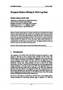
Figure 2. Equivalence classes of itemsets for the dataset D defined in Figure 1.

Definition 5 An itemset I is said to be closed if and only if c(I) = f (g(I)) = f ◦ g(I) = I Now we can define a set of equivalence classes over the lattice of frequent itemsets, where two itemsets X, Y belong to the same class if and only if c(X) = c(Y ), i.e. they have the same closure. Closed itemsets are exactly the maximal elements of these equivalence classes. Figure 2 shows the lattice of frequent itemsets derived from the same simple dataset of Figure 1. Each equivalence class contains elements sharing the same supporting transactions, and closed itemsets are their maximal elements. In this situation we have that Cl (FTh D (Cfreq[D,3] )) = {habc, 3i, hbc, 6i, hbcd, 4i, hbcde, 3i, hbce, 4i}. Note that the number of closed frequent itemsets (5) is much less than the number of frequent itemsets (19). It trivially holds that these equivalence classes of frequency are never cut by the border of frequency (as shown in Figure 2); but what happens to these equivalence classes when they are cut by some CAM or CM constraints? In the next Section by giving an answer to this question, we provide a characterization of MP 5 .

3. Closing Theories of Constraints Recall the mining query discussed in the Introduction: Q : Cf req (X) ∧ Cclose (X) ∧ sum(X.price) ≤ 22 The two different interpretations of Q are as follows (where CAM ≡ sum(X.price) ≤ 22): • I1 :

Cl (FTh D (Cfreq[D,σ] )) ∩ FTh D (CAM )

• I2 :

Cl (FTh D (Cfreq[D,σ] ∧ CAM ))

We now prove that these two different interpretations lead to different results sets.

abcde1

abcd 2

abc3

ab

abce 2

2

2

2

ac 3

2

2

a

b6

abde 1

2

c6

Ø

abcde1

Cfreq acde 1

CAM

bcde 3

1

4

bce 4

4

cd 4

4

d4

3

e4

Itemset

SUPPORT

abce 2

abde 1

acde 1

bcde 3

cde 3

abc3

abd2

acd2

abe2

ace 2

ade1

bcd4

bce 4

bde3

cde 3

de 3

ab 3

3

2

2

bc 6

bd 4

4

4

4

de 3

Equivalence Class

xyz3

abcd 2

Cfreq CM

Closed Itemset

(a)

xyz 3

a3

b6

c 6

Ø

d4

e4

Itemset

Equivalence Class

xyz3

SUPPORT

Closed Itemset

xyz 3

(b)

Figure 3. Equivalence classes of frequency when intersected by a C AM (a), and by a CM (b) constraint. Example 1 In Figure 3(a) we show the usual itemsets lattice with the frequency equivalence classes and the border of the theory of CAM ≡ sum(X.price) ≤ 22. In this situation we have that I1 = {hbc, 6i} while on the other hand I2 = {hac, 3i, hbc, 6i, hbd, 4i, hcd, 4i, hce, 4i hcde, 3i}. What has happened is that some equivalence classes have been cut by the CAM constraint. With interpretation I1 we mine closed frequent itemsets and then we remove those ones which do not satisfy the CAM constraint: this way we lose the whole information contained in those equivalence classes cut by the CAM constraint. On the other hand, according to interpretation I2 , we mine the set of itemsets which satisfy the CAM constraint and then we compute the closure of such itemsets collection: thus, by definition, the itemsets bd and cd are solutions because they satisfy CAM and they have not a superset in the result set with the same support and satisfying the constraint. Which one of the two different interpretations is the most reasonable? It is straightforward to see that interpretation I1 is not a condensed representation since it loses a lot of information. In extreme cases it could output an empty solutions set even if there are many frequent itemsets which satisfy the given set of user-defined constraints. On the other hand, interpretation I2 , which corresponds to the definition Cl (FTh D (Cfreq[D,σ] ∧ CAM )), is a concise and lossless representation of FTh D (Cfreq[D,σ] ∧ CAM ). Observe that I2 is a superset of I1 : it contains all closed itemsets which are under the CAM border (as I1 ), plus those itemsets which arise in equivalence classes which are cut by the CAM border (such as for instance ce and cde in Figure 3(a)). Proposition 3 Cl (FTh D (Cfreq ∧ CAM )) ⊇ Cl (FTh D (Cfreq )) ∩ FTh D (CAM )

Let us move to the dual problem. In Figure 3(b) we show the usual equivalence classes and how they are cut by CM ≡ sum(X.prices) ≥ 33. Since CM constraints are upward closed, we have no problems with classes which are cut: the maximal element of the equivalence class will be in the alive part of the class. In other words when we have a CM constraint, the two interpretations I1 and I2 correspond. Proposition 4 Cl (FTh D (Cfreq ∧ CM )) = Cl (FTh D (Cfreq )) ∩ FTh D (CM )

The unique problem that we have with this condensed representation, is that, when reconstructing FTh D (Cfreq[D,σ] ∧ CM ) from it we must take care of testing itemsets which are subsets of elements in Cl (FTh D (Cfreq ∧ CM )) against CM , in order not to produce itemsets which are below the monotone border B + (Th(CM )). Note that, however, we do not need to access the transaction dataset D anymore. Since we mine maximal itemsets of the equivalence classes it is impossible to avoid this problem, unless we store, together with our condensed representation, the border B + (Th(CM )) even if it does not contain any closed itemset. This could be an alternative. However, since closed itemsets provide a much more meaningful set of association rules, we consider a good tradeoff among performance, conciseness and meaningfulness the use of Cl (FTh D (Cfreq ∧CM )) as condensed representation. Finally, if we use free sets instead of closed, we only shift the problem leading to a symmetric situation. Using free sets interpretations I1 and I2 coincide when dealing with anti-monotone constraints because minimal elements are not cut off by the constraint (e.g. de in Fig. 3(a)), but I1 is lossy when dealing with monotone constraints (e.g. no free solution itemsets in Fig. 3(b)).

4. Algorithms In this Section we study algorithms for the computation of MP 5 . We first discuss separately how monotone and anti-monotone constraints can be pushed in the computation, then we show how they can be exploited together by introducing the CCIMiner algorithm.

more efficient when mining closed itemsets, and since FP-Bonsai has proven to be more efficient than ExAMiner, we decide here to use a FP-growth based depthfirst strategy for the mining problem MP 5 . Thus we combine Closet [16], which is the FP-growth based algorithm for mining closed frequent itemset, with FPBonsai, which is the FP-growth based algorithm for mining frequent itemset with CM constraints.

4.1. Pushing Monotone Constraints

4.2. Pushing Anti-monotone Constraints

Pushing CAM constraints deep into the frequent itemset mining algorithm (attacking the problem FTh D (Cfreq[D,σ] ∧ CAM )) is easy and effective [13], since they behave exactly as Cfreq . The case is different for CM constraints, since they behave exactly the opposite of frequency. Indeed, CAM constraints can be used to effectively prune the search space to a small downward closed collection, while the upward closed collection of the search space satisfying the CM constraints cannot be exploited at the same time. This tradeoff holding on the search space of the computational problem FTh D (Cfreq[D,σ] ∧ CM ) has been extensively studied [18, 9, 4], but all these studies have failed to find the real synergy of these two opposite types of constraints, until the recent proposal of ExAnte [6]. In that work it has been shown that a real synergy of the two opposites exists and can be exploited by reasoning on both the itemset search space and the transactions input database together. According to this approach each transaction can be analyzed to understand whether it can support any solution itemset, and if it is not the case, it can be pruned. In this way we prune the dataset, and we get the fruitful side effect to lower the support of many useless itemsets, that in this way will be pruned because of the frequency constraint, strongly reducing the search space. Such approach is performed with two successive reductions: µ-reduction (based on monotonicity) and α-reduction (based on anti-monotonicity). According to µ-reduction we can delete transactions which do not satisfy CM , in fact no subset of such transactions satisfies CM and therefore such transactions cannot support any solution itemsets. After such reduction, a singleton item may happen to become infrequent in the pruned dataset, an thus it can be deleted by the αreductions. Of course, these two step can be repeated until a fixed point is reached, i.e. no more pruning is possible. This simple yet very effective idea has been generalized in an Apriori-like breadth-first computation in ExAMiner [5], and in a FP-growth [10] based depth-first computation in FP-Bonsai [7]. Since in general depth-first approaches are much

Anti-monotone constraints CAM can be easily pushed in a Closet computation by using them in the exact same way as the frequency constraint, exploiting the downward closure property of antimonotone constraints. During the computation, as soon as a closed itemset X s.t. ¬ CAM (X) is discovered, we can prune X and all its supersets by halting the depth first visit. But whenever, such closed itemset X s.t. ¬ CAM (X) is met (e.g. bcd in Figure 3(a)), some itemsets Y ⊂ X belonging to the same equivalence class and satisfying the constraint may exist (e.g. bd and cd in Figure 3(a)). For this reason we store every such X in a separate list, named Edge, and after the mining we can reconstruct such itemsets Y by means of a simple top-down process, named Backward-Mining, described in Algorithm 1. Algorithm 1 Backward-Mining Input: Edge, C, CAM , CM // C is the set of frequent closed itemsets // CAM is the antimonotone constraint // CM is a monotone constraint (if present) Output: MP 5 1: MP 5 = C; // split Edge by cardinality 2: k = 0; 3: for all c ∈ Edge s.t. CM (c) do 4: E|c| = E|c| ∪ {c}; 5: if (k < |c|) then 6: k=c; // generate and test subsets 7: for (i = k; i > 1; i − −) do 8: for all c ∈ E|i| s.t. CM (c) do 9: for all (i − 1)-subset s of c do 10: if (¬∃Y ∈ MP 5 | s ⊆ Y ) then 11: if CAM (s) then 12: MP 5 = MP 5 ∪ s; 13: else 14: E|i−1| = E|i−1| ∪ s; The backward process in Algorithm 1, generates level-wise every possible subset starting from the bor-

der defined by Edge without getting into equivalence classes which have been already mined (Line 10). If such subset satisfies the constraint then it can be added to the output (Line 12), otherwise, it will be reused later to generate new subsets (Line 14). If we have a monotone constraint in conjunction, the backward process is stopped whenever the monotone border B + (Th(CM )) is reached (Lines 3 and 8).

1. the recursion is stopped whenever an itemset is found to violate the anti-monotone constraint CAM (Line 2); 2. µ and α reductions are merged in to the computation by pruning every projected conditional FPTree (as done in FP-Bonsai [7]) (Lines 11-16); 3. the Backward-Mining has to be performed to retrieve closed itemsets of those equivalence classes which have been cut by CAM (Line 22).

4.3. Closed Constrained Itemsets Miner The two techniques which have been discussed above are independent. We push monotone constraints working on the dataset, and anti-monotone constraints working on the search space. It’s clear that these two can coexist consistently. In Algorithm 2 we merge them in a Closet-like computation obtaining CCIMiner. Algorithm 2 CCIMiner Input: X, D |X , C, Edge, MP 5 , CAM , CM // X is a closed itemset // D |X is the conditional dataset // C is the set of closed itemsets visited so far // Edge set of itemsets to be used in the BackwardMining // MP 5 solution itemsets discovered so far // CAM , CM constraints Output: MP 5 1: C = C ∪ X 2: if ¬CAM (X) then 3: Edge = Edge ∪ X 4: else 5: if CM (X) then 6: MP 5 = MP 5 ∪ X 7: for all i ∈ flist (D |X ) do 8: I = X ∪ {i} // new itemset // avoid duplicates 9: if ¬∃Y ∈ C | I ⊆ Y ∧ supp(I) = supp(Y ) then 10: D |I = ∅ // create conditional fp-tree 11: for all t ∈ D |X do 12: if CM (X ∪ t) then 13: D |I = D |I ∪{t |I } // µ-reduction 14: for all items i occurring in D |I do 15: if i ∈ / flist (D |I ) then 16: D |I = D |I \i // α-reduction 17: for all j ∈ flist (D |I ) do 18: if sup D|I (j) = sup(I) then 19: I = I ∪ {j} // accumulate closure 20: D |I = D |I \{j} 21: CCIM iner(I, D |I , C, B, MP 5 , CAM , CM ) 22: MP 5 = Backward-Mining(Edge, MP 5 , CAM , CM ) For the details about FP-Growth and Closet see [10, 16]. Here we want to outline three basic steps:

5. Experimental Results The aim of our experimentation is to measure performance benefits given by our framework, and to quantify the information gained w.r.t. the other lossy approaches. All the tests were conducted on a Windows XP PC equipped with a 2.8GHz Pentium IV and 512MB of RAM memory, within the cygwin environment. The datasets used in our tests are those ones of the FIMI repository1 , and the constraints were applied on attribute values (e.g. price) randomly generated with a gaussian distribution within the range [0, 150000]. In order to asses the information loss of the postprocessing approach followed by previous works, in Figure 4(a) we plot the difference in cardinality of the solution sets given by two interpretations, i.e. |I2 \ I1 |. On both datasets PUMBS and CHESS this difference rises up to 105 itemsets, which means about the 30% of the solution space cardinality. It is interesting to observe that the difference is larger for medium selective constraints. This seems quite natural since such constraints probably cut a larger number of equivalence classes of frequency. In Figure 4(b) the number of FP-tree data structures built during the mining is reported. On every dataset tested, the number of FP-trees decrease of about four orders of magnitude with the increasing of the selectivity of the constraint. This means that the technique is quite effective independently of the dataset. Finally, in Figure 4(c) we plot run-time comparison of our algorithm CCIMiner w.r.t. Closet at different selectivity of the constraint. Since the post-processing approach must first compute all closed frequent itemsets, we can consider Closet execution-time as a lowerbound on the post-processing approach performance. Recall that CCIMiner exploits both requirements (satisfying constraints and being closed) together at mining time. This exploitation can give a speed up of about to two orders of magnitude, i.e. from a factor 6 with the dataset CONNECT, to a factor of 500 with the dataset CHESS. Obviously the performance improvements become stronger as the constraint become more selective. 1

http://fimi.cs.helsinki.fi/data/

Information loss

Number of FP-trees generated

6

Run time performance 4

7

10

10

10

5

6

10

10

3

10 4

5

10

3

!I2\I1|

10

2

execution time (sec.)

number of fp-trees

10

4

10

2

10

3

10

10

1

10 1

10

PUMSB@29000 CHESS @ 1200

0

10

CCI Miner closet CCI Miner closet CCI Miner closet

2

10

0

2

4

6

8 m

10

12

PUMSB @ 29000 CHESS @ 1200 CONNECT@11000

1

14

10

0

0.2

0.4

0.6

5

x 10

(a)

0.8

1 m

1.2

1.4

1.6

0

1.8

2

10

0

2

6

x 10

(b)

4

6

8 m

10

(PUMSB @ 29000) (PUMSB @ 29000) (CHESS @ 1200) (CHESS @ 1200) (CONNECT @ 11000) (CONNECT @ 11000) 12

14

(c)

Figure 4. Experimental results with CAM ≡ sum(X.price) ≤ m.

6. Conclusions In this paper we have addressed the problem of mining frequent constrained closed patterns from a qualitative point of view. We have shown how previous works in literature overlooked this problem by using a postprocessing approach which is not lossless, in the sense that the whole set of constrained frequent patterns cannot be derived. Thus we have provided an accurate definition of constrained closed itemsets w.r.t the conciseness and losslessness of this constrained representation, and we have deeply characterized the computational problem. Finally we have shown how it is possible to quantitative push deep both requirements (satisfying constraints and being closed) into the mining process gaining performance benefits with the increasing of the constraint selectivity.

References [1] R. Agrawal, T. Imielinski, and A. N. Swami. Mining association rules between sets of items in large databases. In Proceedings ACM SIGMOD, 1993. [2] R. Agrawal and R. Srikant. Fast Algorithms for Mining Association Rules in Large Databases. In Proceedings of the 20th VLDB, 1994. [3] R. J. Bayardo. Efficiently mining long patterns from databases. In Proceedings of ACM SIGMOD, 1998. [4] F. Bonchi, F. Giannotti, A. Mazzanti, and D. Pedreschi. Adaptive Constraint Pushing in frequent pattern mining. In Proceedings of 7th PKDD, 2003. [5] F. Bonchi, F. Giannotti, A. Mazzanti, and D. Pedreschi. ExAMiner: Optimized level-wise frequent pattern mining with monotone constraints. In Proc. of ICDM, 2003. [6] F. Bonchi, F. Giannotti, A. Mazzanti, and D. Pedreschi. Exante: Anticipated data reduction in constrained pattern mining. In Proceedings of the 7th PKDD, 2003. [7] F. Bonchi and B. Goethals. FP-Bonsai: the art of growing and pruning small fp-trees. In Proc. of the Eighth PAKDD, 2004.

5

x 10

[8] J. Boulicaut and B. Jeudy. Mining free itemsets under constraints. In International Database Engineering and Applications Symposium (IDEAS), 2001. [9] C. Bucila, J. Gehrke, D. Kifer, and W. White. DualMiner: A dual-pruning algorithm for itemsets with constraints. In Proc. of the 8th ACM SIGKDD, 2002. [10] J. Han, J. Pei, and Y. Yin. Mining frequent patterns without candidate generation. In Proceedings of ACM SIGMOD, 2000. [11] L.Jia, R. Pei, and D. Pei. Tough constraint-based frequent closed itemsets mining. In Proc.of the ACM Symposium on Applied computing, 2003. [12] H. Mannila and H. Toivonen. Multiple uses of frequent sets and condensed representations: Extended abstract. In Proceedings of the 2th ACM KDD, page 189, 1996. [13] R. T. Ng, L. V. S. Lakshmanan, J. Han, and A. Pang. Exploratory mining and pruning optimizations of constrained associations rules. In Proc. of SIGMOD, 1998. [14] N. Pasquier, Y. Bastide, R. Taouil, and L. Lakhal. Discovering frequent closed itemsets for association rules. In Proceedings of 7th ICDT, 1999. [15] J. Pei, J. Han, and L. V. S. Lakshmanan. Mining frequent item sets with convertible constraints. In (ICDE’01), pages 433–442, 2001. [16] J. Pei, J. Han, and R. Mao. CLOSET: An efficient algorithm for mining frequent closed itemsets. In ACM SIGMOD Workshop on Research Issues in Data Mining and Knowledge Discovery, 2000. [17] J. Pei, J. Han, and J. Wang. Closet+: Searching for the best strategies for mining frequent closed itemsets. In SIGKDD ’03, August 2003. [18] L. D. Raedt and S. Kramer. The levelwise version space algorithm and its application to molecular fragment finding. In Proc. IJCAI, 2001. [19] R. Srikant, Q. Vu, and R. Agrawal. Mining association rules with item constraints. In Proceedings ACM SIGKDD, 1997. [20] M. J. Zaki and C.-J. Hsiao. Charm: An efficient algorithm for closed itemsets mining. In 2nd SIAM International Conference on Data Mining, April 2002.