(n2,q2) the horizontal composition S1 â³S2 is defined only if n1 = m2 and the type ..... if (C) then P1 else P2 is constructed, for a condition C involving both, the.
On Compiling Structured Interactive Programs with Registers and Voices� Cezara Dragoi�� and Gheorghe Stefanescu Faculty of Mathematics and Computer Science, University of Bucharest Str. Academiei 14, Bucharest, Romania 010014 {cdragoi,gheorghe}@funinf.cs.unibuc.ro
Abstract. A model (consisting of rv-systems), a core programming language (for developing rv-programs), several specification and analysis techniques appropriate for modeling, programming and reasoning about interactive computing systems have been recently introduced by Stefanescu using register machines and space-time duality, see [13]. In [3,4,5,6] the authors have have introduced and studied structured programming techniques for rv-systems. The aim of the present paper is to define a scenario-based operational semantics for structured rv-programs and to offer a translation from structured rv-programs to rv-programs. The main technical result states that the translation is correct. This is part of an effort to get a running environment for structured rv-programs built up on top of rv-programs. Keywords: interactive systems, structured rv-systems, programming languages, operational semantics, registers and voices, compiler correctness.
1
Introduction
Interactive computation has a long tradition and there are many successful approaches to deal with the intricate aspects of this type of computation, see [1,2,7,8,15], to mention just a few references from a very rich literature. However, a general simple and unifying model for interactive computation, extending the classical, popular imperative programming paradigm, is still to be find. A model (consisting of rv-systems), a core programming language (for developing rv-programs), several specification and analysis techniques appropriate for modeling, programming and reasoning about interactive computing systems have been recently introduced by Stefanescu using register machines and spacetime duality, see [13]. One of the key features of the model is the introduction of high-level temporal data structures. Actually, having high level temporal data on interaction interfaces is of crucial importance in getting a compositional model �
��
This research was partially supported by the Romanian Ministry of Education and Research (PNCDI-II Program 4, Project D1/1052/18.09.2007: GlobalComp - Models, semantics, logics and technologies for global computing). Current address: LIAFA, Universite Paris Diderot - Paris 7, France.
V. Geffert et al. (Eds.): SOFSEM 2008, LNCS 4910, pp. 259–270, 2008. c Springer-Verlag Berlin Heidelberg 2008 �
260
C. Dragoi and G. Stefanescu
for interactive systems, a goal not always easy to achieve (recall the difficulties in getting a compositional semantics for data-flow networks). In [3,4,5] the authors have introduced and studied structured programming techniques for rv-systems. In [6], a kernel programming language for interactive systems AGAPIA is introduced and its typing system is studied. See [14,10] for more information and results on rv-systems and their verification. The aim of the present paper is to offer a translation from structured rvprograms to rv-programs. This is part of an effort to get a running environment for structured rv-programs built up on top of rv-programs. The main technical contribution of the paper is a proof of the translation correctness. The paper is organized as follows. It start with a presentation of spatial and temporal data, of spatio-temporal relational specifications, and of scenarios and operations on scenarios. Next, after a brief recall of rv-programs, structured rvprograms are introduced. Then, the scenario-based operational semantics is presented. After that, the translation from structured rv-programs to rv-programs is defined and finally, the statement on translation correctness is included. (The proof of the translation correctness, developed in the long version of the paper, is rather tricky, based on a good understanding of rv-program transformations.)
2
Scenarios
In this section we briefly present temporal data, spatio-temporal specifications, grids, scenarios, and operations on scenarios. 2.1
Specifications and Scenarios
Spatio-temporal specifications. To handle spatial data, common data structures and their natural representations in memory are used. For the temporal data, we use streams: a stream is a sequence of data ordered in time and is denoted as a0 � a1 � . . ., where a0 , a1 , . . . are its data at time 0, 1, . . ., respectively. Typically, a stream results by observing the data transmitted along a channel: it exhibits a datum (corresponding to the channel type) at each clock cycle. A voice is defined as the time-dual of a register: A voice is a temporal data structure that holds a natural number. It can be used (“heard”) at various locations. At each location it displays a particular value. Voices may be implemented on top of a stream in a similar way registers are implemented on top of a Turing tape, for instance specifying their starting time and their length. Most of usual data structures have natural temporal representations. Examples include timed booleans, timed integers, timed arrays of timed integers, etc. For an interactive system using no more complex data than registers and voices, a spatio-temporal specification S : (m, p) → (n, q) is a relation S ⊆ (Nm × Np ) × (Nn × Nq ), where m (resp. p) is the number of input voices (resp. registers) and n (resp. q) is the number of output voices (resp. registers). It may be defined as a relation between tuples, written as �v | r� �→ �v � | r� �, where v, v � (resp. r, r� ) are tuples of voices (resp. registers).
On Compiling Structured Interactive Programs with Registers and Voices
261
Specifications may be composed horizontally and vertically, as long as their types agree; e.g., for two specifications S1 : (m1 , p1 ) → (n1 , q1 ) and S2 : (m2 , p2 ) → (n2 , q2 ) the horizontal composition S1 � S2 is defined only if n1 = m2 and the type of S1 � S2 is (m1 , p1 + p2 ) → (n2 , q1 + q2 ). Grids and scenarios. A grid is a rectangular two-dimensional area filled in with letters of a given alphabet. An example of a grid is presented in Fig. 1(a). In our standard interpretation, the columns correspond to processes, the top-to-bottom order describing their progress in time. The left-to-right order corresponds to process interaction in a nonblocking message passing discipline: a process sends a message to the right, then it resumes its execution. (See [9] for related studies.) A scenario is a grid enriched with data around each letter. The data may have various interpretation: they either represent control/interaction information, or current data of the variables, or both. Fig. 1 illustrates the first case, Fig. 1(c) the last case, and Fig. 1(d) the middle case. Notice that the scenario from Fig. 1(d) is similar to that in (c), but the control/interaction labels A,B,C,1,2,3 are omitted. The scenarios of a rv-program look like in (c), while those of structured rvprograms as in (d) - there are not labels in the latter case. 1: x=4 A:
aabbabb abbcdbb bbabbca ccccaaa
1 1 1 AaBbBbB 2 1 1 AcAaBbB 2 2 1 AcAcAaB 2 2 2
(a)
(b)
1: y=nil
1: z=nil
B: C: D X tx=4 Y Z 3: 2: 2: x=2 y=4 z=4 A: B: C: D U tx=2 V W 3: 2: 2: x=1 z=2 A: B: C: D: U tx=1 V W 2: 2: 2: x=0 z=0 (c)
x=4 tx=4 tx=4 Y Z X x=2 y=4 z=4 tx=2 tx=2 U V W x=1 y=4 z=2 (d)
Fig. 1. A grid (a), an abstract scenario (b), and concrete scenarios (c,d)
The type of a scenario interface of type (d) is represented as t1 ; t2 ; . . . ; tk , where each tk is a tuple of simple types used in the scenario cells. An empty tuple is also written 0 or nil and can be freely inserted to or omitted form such descriptions. The type of a scenario f is specified by the notation f : �w|n� → �e|s�, where w/n/e/s represent the types of its west/north/east/south borders. For the example in Fig. 1(d), the type is �nil; nil|sn; nil; nil� → �nil; nil|sn; sn; sn�, where sn denotes the spatial integer type. 2.2
Operations with Scenarios
We say two scenario interfaces t = t1 ; t2 ; . . . ; tk and t� = t�1 ; t�2 ; . . . ; t�k� are equal if k = k � and the types and the values of each pair ti , t�i are equal. Two interfaces
262
C. Dragoi and G. Stefanescu
a d g
b e h
c f i
A
A
nil
B
B
X
b
c
d
e
f
g
h
i
Y
Z
U
nil V
(a)
a
W
(b)
A
X
Y
Z
U
nil V
W
nil B
(c)
Fig. 2. Horizontal composition of scenarios
are equal up to the insertion of nil elements, written t =n t� , if one can insert nil elements into these interfaces such that the resulting interfaces are equal. We denote by Idm,p : �m|p� → �m|p� the identity constant, i.e., the temporal/spatial output is equal to the temporal/spatial input, respectively. Horizontal composition: Suppose we start with two scenarios fi : �wi |ni � → �ei |si �, i = 1, 2. Their horizontal composition f1 � f2 is defined only if e1 =n w2 . For each inserted nil element in an interface, a dummy row is inserted in the corresponding scenario, resulting a scenario fi . After these transformations, the result is obtained putting f1 on left of f2 . (Notice that f1 : �w1 |n1 � → �t|s1 � and f2 : �t|n2 � → �e2 |s2 �, where t is the resulting common interface.) The result, f1 � f2 : �w1 |n1 ; n2 � → �e2 |s1 ; s2 �, is unique up to insertion or deletion of dummy rows. See Fig. 2 and Fig. 3(b). Its identities are Idm,0 . Vertical composition The definition of vertical composition f1 ·f2 is similar, but now s1 =n n2 . For each inserted nil element, a dummy column is inserted in the corresponding scenario, resulting a scenario fi . The result, f1 ·f2 : �w1 ; w2 |n1 � → �e1 ; e2 |s2 �, is obtained putting f1 on top of f2 . See Fig. 3(a). Its identities are Id0,m . Constants: Except for the already defined identities I, additional constants may be used. Some of them may be found in Fig. 3: A recorder R (2nd cell in the 1st row of (c)), a speaker S (1st cell in the 2nd row of (c)), an empty cell Λ (3rd cell in the 1st row of (c)), etc. Diagonal composition: The diagonal composition f1 • f2 is defined only if e1 =n w2 and s1 =n n2 . It is a derived operation defined by f1 • f2 = (f1 � R1 � Λ1 ) · (S2 � Id � R2 ) · (Λ2 � S1 � f2 ) for appropriate constants R, S, Id, Λ. See Fig. 3(c). In this case R1 : �t| � → � |t�, S1 : � |t� → �t| �, Id : �u|t� → �u|t�, R2 : �u| � → � |u�, S2 : � |u� → �u| �, where
X X X Y
(a)
(d)
Y (b)
(c)
Y
Fig. 3. Operations on scenarios
(f)
(e)
(g)
On Compiling Structured Interactive Programs with Registers and Voices
263
t (resp. u) is a common representation for e1 and w2 (resp. s1 and n2 ) obtained inserting nil elements. Its identities are Idm,n . We extend the definitions of the scenario compositions to set of scenarios. Given two sets of scenarios, A and B, we define the horizontal composition A � B = {fa � fb | for fa ∈ A and fb ∈ B}. The vertical composition A · B and the diagonal composition A • B on set of scenarios A, B are similarly defined.
3
Rv-Programs
In this section we briefly describe rv-programs (interactive programs with registers and voices); see [13,14] for more details. Finite interactive systems. A finite interactive system (shortly fis) is a finite hyper-graph with two types of vertices and one type of (hyper) edges: the first type of vertices is for states (labeled by numbers), the second is for classes (labeled by capital letters) and the edges/transitions are labeled by letters denoting the atoms of the grids; each transition has two incoming arrows (one from a class and the other from a state), and two outgoing arrows (one to a class and the other to a state). Some classes/states may be initial (indicated by small incoming arrows) or final (indicated by double circles); see, e.g., [12,13]. An example is shown below. For the parsing procedure, given a fis F and a grid w, insert initial states/classes at the north/west border of w and parse the grid completing the scenario according to the fis transitions; if the grid is fully parsed and the south/east border contains final states/classes only, then the grid w is recognized by F . The language of F is the set of its recognized grids. A fis F1 and a parsing accepting abb cab are shown cca
below.
F1 =
1
b
A
a
B
c
2
1 1 1 Aa b b Ac a b Ac c a
1 1 1 1 1 1 AaBb b . . . AaBbBbB 2 2 1 1 Ac a b AcAaBbB 2 2 1 Ac c a AcAcAaB 2 2 2
Interactive programs with registers and voices. An rv-system (interactive system with registers and voices) is a fis enriched with: (i) registers associated to its states and voices associated to its classes; and (ii) appropriate spatio-temporal transformations for actions. We study programmable rv-systems specified using rv-programs. An example of rv-program is presented in Fig. 4. A computation is described by a scenario mixing control/interaction labels and data; see Fig. 1(c) for an example. Syntax of rv-programs. A program is a collection of modules. A module has a name and 4 areas: (1) The top-left part contains a pair of labels specifying the interaction/control (class/state) coordinates where the module may be applied.
264
C. Dragoi and G. Stefanescu
in: A,1; out: D,2 X:: (A,1) x : sInt tx : tInt; tx = x; x = x/2; goto [B,3]; Y:: (B,1) y : sInt tx : y = tx; tInt goto [C,2];
W:: (C,2) z : sInt tx : z = z - tx; tInt goto [D,2];
V:: (B,2) y : sInt tx : if(y%tx != 0) tInt tx = 0; goto [C,2];
U:: (A,3) x : sInt tx : tInt; tx = x; x = x - 1; if (x > 0) {goto [B,3]} else {goto [B,2];} Z:: (C,1) z : sInt tx : z = tx; tInt goto [D,2];
Fig. 4. The rv-program Perfect (for perfect numbers)
(2)-(3) The top-right (resp. bottom-left) part specifies the spatial (resp. temporal) input variables. (4) The bottom-right part is the body of the module, including C-like code. The exit from the module is specified by a goto statement. A statement, say goto [B,3], indicates that: (i) the data of the spatial variables in the current module will be used in a next module with control state 3; and (ii) the data of the temporal variables in the current module will be used for the interaction interface of a new module with interaction label B. Operational and denotational semantics of rv-programs. The operational semantics is given in terms of scenarios. Scenarios are built up with the following procedure, described using the scenario in Fig. 1(c) for the rv-program Perfect: (1) Each cell has a module name as label. (2) In the areas around a cell we show how variables are modified. (3) In a current cell, the values of spatial variables are obtained going vertically up and collecting the last updated values. (4) Similarly, the full information on temporal variables in a current cell is obtained collecting their last updated values going horizontally on left. (5) The first column has input classes and particular values for their temporal variables; the first row has input states and particular values for their spatial variables. (6) The computation in a cell α is done as follows: (i) Take a module β of the program bearing the class label of the left neighboring area of α and the state label of the top neighboring area of α. (ii) Follow the code in β using the spatial and the temporal variables of α with their current values. (iii) If the local execution of β is finished with a goto [Γ, γ] statement, then the label of the right neighboring area of α is set to Γ and the label of the bottom neighboring area of α is set to γ. (iv) Insert the values of the temporal variables updated by β in the right neighboring area of α and the values of the spatial variables updated by β in the bottom neighboring area of α. (7) A partial scenario (for an rv-program) is a scenario built up using the above rules; it is a complete scenario if the bottom row has only final states and the rightmost column has only final classes.
On Compiling Structured Interactive Programs with Registers and Voices
265
The scenario in Fig. 1(c) is a complete scenario for the rv-program Perfect. The input-output denotation of an rv-program is the relation between the input data on the north/west borders and output data on the south/east borders of the program scenarios. Notice that a global scoping rule is implicitly used here: once defined, a variable is always available. It is also possible to introduce rv-programs obeying a stronger typing discipline, where each module comes with an explicit type at each border. This option is actually used for structured programs to be introduced in the next section.
4
Structured rv-Programs
The rv-programs, briefly presented in the previous section, resemble flowcharts and assembly languages: one freely uses goto statements, with both temporal and spatial labels. The aim of this section is to introduce structured programming techniques on top of rv-programs. The resulting structured rv-programs may be described directly, from scratch. The lower level of rv-programs is used as a target language for compiling. 4.1
Syntax, Examples
The syntax of structured rv-programs. It is given by the BNF grammar P::= X | if (C)then{P }else{P }| P %P | P #P | P $P | while t(C){P } | while s(C){P }| while st(C){P } X::= module{listen t vars}{read s vars}{ code; }{speak t vars}{write s vars} Structured rv-programs use modules X as their basic blocks. On top of them, larger programs are built up by “if” and composition and iteration constructs for the vertical (or temporal), the horizontal (or spatial), and the diagonal (or spatio-temporal) directions, i.e., (%, while t)/(#, while s)/($, while st). These statements aim to capture at the program level the corresponding operations on scenarios. Examples. We include a simple, but rather general example of structured rvprogram to give a clue to the reader on the naturalness and the expressiveness of the language. More examples may be found, e.g., in [3,5,10]. A structured rv-program for a ring termination detection protocol is presented in [5]; except for the details on I1,I2,R, it has the following format P :: [I1# for s(tid=0;tid