Apr 18, 2006 - enjoys the same property for every n ⥠3; the orbits are inscribed ... wants to describe plane billiards such that the billiard ball map has an .... We also prove that, for every outer billiard table, the set of 3-periodic ..... Assume that Ëγ0(t) lies in the kernel of the restriction of Ï(λ) on the fiber ... its center of mass.
arXiv:math/0604388v1 [math.DG] 18 Apr 2006
On configuration spaces of plane polygons, sub-Riemannian geometry and periodic orbits of outer billiards Daniel Genin and Serge Tabachnikov Department of Mathematics, Penn State University University Park, PA 16802, USA
1
Introduction
The classical billiard system describes the motion of a point in a plane domain subject to the elastic reflection off the boundary, described by the familiar law of geometrical optics: the angle of incidence equals the angle of reflection; see, e.g., [13, 14] for surveys of mathematical billiards. For every n ≥ 2, the billiard system inside a circle has a very special property: every point of the circle is the starting point of an n-periodic billiard orbit; this orbit is an inscribed regular n-gon.1 Likewise, an ellipse enjoys the same property for every n ≥ 3; the orbits are inscribed n-gons of extremal perimeter length.2 A billiard table of constant width also has the property that every point on its boundary belongs to a 2-periodic, back-andforth, billiard trajectory, and this is a dynamic characterization of the curves of constant width. The phase space of the billiard ball map is a cylinder, and the family of n-periodic orbits forms an invariant circle of the billiard ball map consisting of n-periodic points. How exceptional is this property? More specifically, given n ≥ 3, one wants to describe plane billiards such that the billiard ball map has an invariant curve consisting of n-periodic points. The first result in this direc1
Similarly, one can consider periodic orbits with other rotation numbers corresponding to regular star-shaped polygons. 2 For circles and ellipses, this behavior is due to the complete integrability of the billiard ball map.
1
tion was obtained by Innami [8]: he constructed a billiard curve, other than a circle or an ellipse, whose every point is a vertex of a 3-periodic billiard trajectory (these billiard triangles are isosceles in his example).3 In a recent paper [1], Baryshnikov and Zharnitskii developed a new elegant approach to this problem. In a nutshell, their innovation was in switching focus from billiard curves to the space of plane n-gons. If such an n-gon, z1 , . . . , zn , is a periodic billiard trajectory then, due to the law “the angle of incidence equals the angle of reflection”, we know the directions of the billiard curve at each vertex zi . This determines an n-dimensional distribution D in the space of n-gons, called the Birkhoff distribution. One can further restrict attention to the hypersurface of n-gons with a fixed perimeter length: the Birkhoff distribution is everywhere tangent to these hypersurfaces. It turns out that the Birkhoff distribution is non-integrable. A 1-parameter family of billiard n-gons z1 (t), . . . , zn (t), 0 ≤ t ≤ 1, is interpreted as a curve in the space of n-gons, tangent to D and satisfying the “monodromy” condition zi (1) = zi+1 (0), i = 1, . . . , n. The problem of finding such horizontal curves belongs to sub-Riemannian geometry and non-holonomic dynamics. The main result of [1] is that, for every n ≥ 2, the space of billiard tables, for which the billiard ball map possesses an invariant curve consisting of n-periodic points, is infinite-dimensional (this space also has an infinite codimension in the space of all billiard tables). Example 1.1 Let us illustrate this approach in the simplest case n = 2, that is, curves of constant width (for information on billiards of constant width, see [9]). Consider the space of oriented segments, say, of length 2. A segment z1 z2 is “allowed” to move in such a way that the velocities of both end-points are orthogonal to the segment. Let O = (x, y) be the mid-point of the segment and α its direction. Then the space of segments has coordinates (x, y, α) and z1 = (x − cos α, y − sin α), z2 = (x + cos α, y + sin α). We conclude that the velocity of point O must be orthogonal to the vector (cos α, sin α), and this is the definition of the Birkhoff distribution in this case. Thus D is the kernel of the 1-form λ = cos α dx + sin α dy. This 1-form is contact: λ ∧ dλ 6= 0. We have identified our space of segments with the 3
A similar result was obtained by M. Berger, unpublished.
2
space of cooriented contact elements in the plane, a fundamental example of a contact 3-dimensional manifold (see, e.g., [4]). If z1 (t)z2 (t) is a curve, tangent to D and satisfying the monodromy condition z1 (1) = z2 (0), z2 (1) = z1 (0), then the respective curve (x(t), y(t), α(t)) is Legendrian (i.e., tangent to the contact distribution) and satisfies x(1) = x(0), y(1) = y(0) and α(1) = α(0) + π. The projection of this Legendrian curve on the (x, y)-plane, that is, the trajectory of the mid-point O, is a closed smooth curve ∆ with singularities (generically, semi-cubical cusps); the total winding of this curve is π. Every such curve ∆ uniquely lifts to a Legendrian curve in the space of contact elements: the missing α coordinate is recovered as the slope: cot α = −dy/dx. In other words, we use ∆ as a guide: place a segment of length 2 so that its mid-point O is on the curve ∆ and the segment is orthogonal to ∆, and then slide the segment around ∆. If certain convexity conditions hold (for example, ∆ should not have inflection points) then the end-points z1 and z2 will describe a curve of constant width. For example, if the end-points z1 and z2 move along a circle then ∆ degenerates to its center, and if z1 and z2 describe the Reuleaux triangle then ∆ is made of three 60◦ arcs of a circle, see figure 1.
Figure 1: Reuleaux triangle and the curve ∆ In this paper we extend the results from [1] to outer (or dual) billiards, a dynamical system that is a close relative of the conventional, inner, billiards; see [3, 13, 14] for surveys and [5] for a recent interesting result. An outer billiard table is a strictly convex compact plane domain D. Pick a point x outside D. There are two support lines from x to D; choose one 3
of them, say, the right one from x’s view-point, and reflect x in the support point. One obtains a new point, y, and the transformation T : x 7→ y is the outer billiard map, see figure 2. If the boundary of the outer billiard table contains straight segments (for example, is a convex polygon), the map T or its inverse is not defined on the lines containing these segments; this still leaves a set of full measure on which all iterations of T are defined. We will consider only outer billiard tables with strictly convex smooth boundaries.
x
T(x) Figure 2: Outer billiard map Let us mention four fundamental properties of outer billiards, important for us. First, the outer billiard map commutes with affine transformations of the plane. Secondly, the outer billiard map preserves the standard area form in the plane (similarly to the billiard ball map which is an area preserving map of a cylinder). Thirdly, the outer billiard map is a twist map of the exterior of the outer billiard table D, a semi-infinite cylinder, with respect to the vertical foliation consisting of tangent half-lines to the boundary of D. And finally, an n-periodic outer billiard orbit is an n-gon (possibly, starshaped), circumscribed about the table D and having an extremal area. This is an outer analog of a variational property of periodic billiard trajectories: they are inscribed polygons of extremal perimeter length. As a consequence, if an outer billiard has a 1-parameter family of n-periodic orbits then the respective circumscribed n-gons have the same areas. Let Gn be the cyclic configuration space of the plane, that is, the space of polygons z1 , . . . , zn such that zi 6= zi+1 for i = 1, . . . , n (where the index i is understood cyclically). If z1 (t), . . . , zn (t) is a 1-parameter family of n-periodic outer billiard orbits with T (zi (t)) = zi+1 (t) then each segment zi (t)zi+1 (t) envelopes the boundary of the outer billiard table and is bisected by the tangency point. This prompts the following definition. Denote by F the n-dimensional distribution in Gn determined by the following condition: the velocities of points z1 , . . . , zn lie in F if, for each 4
i = 1, . . . , n, the motion of the line zi zi+1 is an infinitesimal rotation about the mid-point of the segment zi zi+1 . We call F the dual Birkhoff distribution. The dual Birkhoff distribution is tangent to the level hypersurfaces of the area function, and we can restrict attention to non-degenerate polygons of a fixed non-zero area. On this hypersurface, F is non-integrable: the vector fields, tangent to F , and their first commutators generate the tangent space at every point (see Theorem 1). We are interested in the outer billiard tables possessing invariant curves consisting of n-periodic orbits. Such an invariant curve gives rise to a horizontal curve z1 (t), . . . , zn (t), 0 ≤ t ≤ 1, in Gn satisfying the monodromy condition zi (1) = zi+1 (0), i = 1, . . . , n. If the outer billiard table is a circle (or an ellipse) then, for every pair (n, k) where 3 ≤ n, 1 ≤ k ≤ n/2, and k coprime with n, there is an invariant curve consisting of n-periodic orbits with rotation number k (that is, making k turns around D). We show that, for every such pair (n, k), one can perturb a circle so that the resulting outer billiard still has an invariant curve consisting of n-periodic orbits with rotation number k; the space of such deformations is infinite-dimensional and depends on functional parameters (see Theorem 2). In Section 4, we study the simplest case of n = 3 in detail; this is the closest outer billiard analog of curves of constant width. This case illustrates the general approach by explicit computations. We also discuss a discretization of the problem in which a smooth outer billiard curve is replaced by a polygon. We also prove that, for every outer billiard table, the set of 3-periodic orbits has zero measure (see Theorem 4). For inner billiards, this is a wellknown result having a number of different proofs [11, 12, 15, 16]. We also give different proofs, one of them follows ideas of [16] and another those of [1]. Note that there exist area preserving twist maps of a cylinder whose set of periodic points has a non-empty interior. Let us finish this introduction with a problem: can invariant billiard curves (inner or outer) consisting of periodic points with different periods, or the same period but different rotation numbers, coexist, unless the table is an ellipse? In particular, is it true that the only billiard of constant width, having an invariant curve consisting of 3-periodic points, is a circle?
5
2
Configuration space of plane polygons and the dual Birkhoff distribution
Let us fix some notations. The determinant of two vectors, that is, the crossproduct, is denoted by [ , ]. A generic point in the plane is denoted by z = (x, y). If z1 = (x1 , y1) and z2 = (x2 , y2 ) then z1 dz2 denotes the 1-form x1 dx2 +y1 dy2 . Likewise, [z1 , dz2 ] denotes the 1-form x1 dy2 −y1 dx2 and [dz, dz] the 2-form 2dx ∧ dy. If w = (u, v) is a vector in R2 and z = (x, y) is a point then by w∂z we mean the tangent vector u∂x + v∂y. When working with n-gons, we always understand the indices cyclically, so that i = i + n. For a polygon z1 , . . . , zn , set n X [zi , zi+1 ]; A(z1 , . . . , zn ) = i=1
this is twice the area of the polygon (counted with appropriate multiplicities and signs). Let F be the dual Birkhoff distribution on the space of n-gons defined in Section 1. Let Z = (z1 , . . . , zn ) ∈ Gn be an n-gon and W = (w1 , . . . , wn ) a tangent vector to Gn at Z; the vector wi is the velocity of the vertex zi . Lemma 2.1 F is an n-dimensional distribution. A vector W lies in F if and only if, for all i = 1, . . . , n, one has: [wi + wi+1 , zi+1 − zi ] = 0, that is, the vectors wi + wi+1 and zi+1 − zi are collinear. Proof. To see that F is n-dimensional, view a polygon Z = (z1 , . . . , zn ) ∈ Gn as an ordered collection of n lines L = (z1 z2 , z2 z3 , . . . , zn z1 ). From this dual viewpoint, Gn becomes an open subset in the space Ln of n-tuples of oriented lines in the plane. An infinitesimal rotation of the i-th line zi zi+1 about the mid-point of the segment zi zi+1 determines a tangent vector to Ln at point L, and these vectors are clearly independent for i = 1, . . . , n. It follows that dim F = n. For W to belong to F , the line through points zi + εwi and zi+1 + εwi+1 must pass through the mid-point (zi + zi+1 )/2; here ε is infinitesimal. Thus the linear term in ε of the determinant � � zi+1 − zi zi − zi+1 + εwi+1 , + εwi 2 2 6
vanishes, which is equivalent to [wi + wi+1 , zi+1 − zi ] = 0. 2 An n-gon is called non-degenerate if no three consecutive vertices lie on one line. The set of non-degenerate n-gons is denoted by Un . Clearly, Un is an open subset of Gn . Let us introduce the 1-forms αi = [zi+1 − zi , dzi+1 + dzi ], i = 1, . . . , n. Lemma 2.2 Let Z ∈ Un be a non-degenerate polygon. Then the 1-forms αi are linearly independent at Z and the intersection of their kernels is the fiber F (Z) of F at point Z. Proof. First, we claim that each form αi vanishes on every tangent vector W ∈ F . Indeed, αi (W ) = [zi+1 − zi , wi + wi+1 ], and this is zero, according to Lemma 2.1. P Suppose that a non-trivial linear combination ti αi vanishes at point Z. Then, for every test vector W = (w1 , . . . , wn ), one has: X X X 0= ti [zi+1 − zi , wi + wi+1 ] = ti [zi+1 − zi , wi ] + ti [zi+1 − zi , wi+1 ] = X
[ti (zi+1 −zi ), wi]+
Therefore
X
[ti−1 (zi −zi−1 ), wi ] =
X
[ti (zi+1 −zi )+ti−1 (zi −zi−1 ), wi ].
ti (zi+1 − zi ) + ti−1 (zi − zi−1 ) = 0, i = 1, . . . , n.
(1)
Since the polygon Z is non-degenerate, the vectors zi+1 − zi and zi − zi−1 are linearly independent, and (1) implies that ti = 0 for all i. Since F is n-dimensional and the 1-forms αi are linearly independent, one has: ∩ni=1 Ker αi = F . 2 The next lemma shows that one can restrict attention to the level hypersurfaces of the area function. Lemma 2.3 Every non-zero level hypersurface of the function A is smooth, and the distribution F is tangent to these hypersurfaces.
7
Proof. Let Q : V → V ∗ be a self-adjoint linear operator in a vector space V . Consider the quadratic function F (x) = Q(x) · x on V . Then every non-zero level hypersurface of F is smooth. Indeed, by Euler’s formula, ∇F (x) · x = 2F (x), hence dF does not vanish on a non-zero level hypersurface. The function A is a quadratic form on the space of n-gons, and the first claim follows. One has the equality n X
αi =
i=1
n X i=1
[zi+1 , dzi ] − [zi , dzi+1 ] = −dA,
which implies the second claim. 2 Let us construct a system of n linearly independent vector fields tangent to F . Let Z = (z1 , . . . , zn ) be a non-degenerate polygon. Set ai = [zi − zi−1 , zi+1 − zi ], twice the oriented area of the triangle zi−1 zi zi+1 . Denote by Wk = (w1k , . . . , wnk ) the tangent vector to Un at Z whose i-th component is zero, unless i = k or i = k + 1. For these values of i, one has: wk,k = ak+1 (zk − zk−1 ), wk+1,k = ak (zk+2 − zk+1 ), see figure 3. zk
zk−1
zk+1
zk+2
Figure 3: Tangent vector Wk Lemma 2.4 The vectors W1 , . . . , Wn are linearly independent at every point Z ∈ Un and they span F (Z). 8
Proof. To show that Wk lies in F , it suffices to check that the vector ak+1 (zk −zk−1 )+ak (zk+2 −zk+1 ) is collinear with the vector zk+1 −zk . Indeed, [zk+1 − zk , zk+2 − zk+1 ](zk − zk−1 ) + [zk − zk−1 , zk+1 − zk ](zk+2 − zk+1 ) = [zk − zk−1 , zk+2 − zk+1 ](zk+1 − zk ), which follows from the general identity, valid for any three vectors: [u, v]w + [v, w]u + [w, u]v = 0. Under identification of the space of n-gons with the space of n-tuples of lines Ln , the tangent vector Wk corresponds to a nontrivial infinitesimal rotation of the line zk zk+1 about the mid-point of the segment zk zk+1 . Therefore these vectors are linearly independent and hence span the dual Birkhoff distribution. 2 Now we prove that the the dual Birkhoff distribution is completely nonintegrable. Theorem 1 Let M 2n−1 be the hypersurface in Un consisting of non-degenerate n-gons with a fixed non-zero area. Then the tangent space of M at every point is generated by the vectors fields tangent to F and their first commutators. Thus the bracket growth type of F is (n, 2n − 1) (just like that of the Birkhoff distribution, see [1]). Proof. Consider the vector fields ξk = [Wk−1 , Wk ] (the fields Wi and Wj clearly commute if |i − j| ≥ 2). We want to show that these fields, along with F , span the tangent space to M at every point. According to Lemmas 2.2 and 2.3, the 1-forms α1 , . . . , αn−1 constitute a frame in the conormal space to F at every point Z ∈ M. For k = 1, . . . , n, consider the vector (α1 (ξk ), . . . , αn−1 (ξk )) ∈ Rn−1 . It suffices to show that these n vectors span Rn−1. Since the fields Wk belong to the kernel of each form αi , the Cartan formula implies: αi (ξk ) = dαi (Wk−1 , Wk ). Recall that Z = (z1 , . . . , zn ) with zi = (xi , yi). Let ωi = dxi ∧ dyi , i = 1, . . . , n. We claim that dαi = 2(ωi+1 − ωi ). Indeed, dαi = [dzi+1 − dzi , dzi+1 + dzi ] = [dzi+1 , dzi+1 ] − [dzi , dzi ] = 2(ωi+1 − ωi). 9
Thus we want to show that the vectors ((ω2 − ω1 )(Wk−1, Wk ), . . . , (ωn − ωn−1 )(Wk−1, Wk )) span Rn−1 for k = 1, . . . , n. This will follow if we show that the vectors ω1 (Wk−1 , Wk ), ω2 (Wk−1 , Wk ), . . . , ωn (Wk−1 , Wk ) span Rn for k = 1, . . . , n. But ωi(Wk−1 , Wk ) = 0, unless i = k, and ωk (Wk−1 , Wk ) = ak−1 ak ak+1 6= 0. Thus ωi (Wk−1 , Wk ) is a non-degenerate diagonal matrix, and we are done. 2 Remark 2.5 The dual Birkhoff distribution F on the cyclic configuration space Gn is Lagrangian with respect to the following symplectic structure. The space of oriented lines in the plane, topologically, a cylinder, has a canonical area form (see, e.g., [13, 14]), and the direct product of these forms is a symplectic structure in the space of n-tuples of oriented lines Ln . In the proof of Lemma 2.1, we realized Gn as an open subset in Ln , and this provides a symplectic structure on Gn . Infinitesimal rotations of distinct lines determine symplectically orthogonal tangent vectors to Ln , hence F is Lagrangian. The Lagrangian property of the dual Birkhoff distribution echoes that of the Birkhoff distribution [1].
3
Outer billiards with invariant curves consisting of periodic points
In this section we show that, for every pair (n, k) with 3 ≤ n, 1 ≤ k ≤ n/2 and k coprime with n, there is an abundance of outer billiard tables, possessing invariant curves consisting of n-periodic orbits with rotation number k; such tables are constructed as perturbations of circles. Denote by HF2 the space of parameterized horizontal paths [0, 1] → M (paths tangent to the dual Birkhoff distribution) whose first 2 derivatives are square integrable (one can work with a higher number of derivatives as well). For a polygon Z ∈ M, denote by HF2 (Z) the space of paths starting at Z. Then HF2 (Z) is a Hilbert manifold, see [10]. Let Z be a regular star-shaped n-gon with rotation number k. We have the following result. 10
Theorem 2 The set of (parameterized) outer billiard curves, sufficiently close to a circular one and possessing invariant curves consisting of n-periodic orbits with rotation number k, is a smooth Hilbert submanifold of codimension 2n − 1 in HF2 (Z). Proof. To fix ideas, consider the case of simple periodic n-gons, that is, the case of k = 1. At the end of the proof, we will indicate the small adjustment to be made in the case of k > 1. Start with a circular outer billiard. One has a 1-parameter family of periodic n-gons Z(t) = (z1 (t), . . . , zn (t)) with zj (t) = e2πi(j+t)/n , t ∈ [0, 1]
(2)
circumscribed about the circular table (the table is scaled appropriately). Let σ : Gn → Gn be the cyclic permutation of the vertices of a polygon: σ(z1 , . . . , zn ) = (z2 , . . . , zn , z1 ). Then Z(1) = σ(Z(0)). The family (2) determines a horizontal curve γ0 (t) in Gn whose endpoints are Z(0) and Z(1). Denote by HF2 (Z(0), Z(1)) ⊂ HF2 (Z(0)) the set of horizontal curves with the terminal point Z(1). We want to perturb γ0 (t) in HF2 (Z(0), Z(1)). If a perturbation is sufficiently small and trivial in a neighborhood of end-points then we obtain a 1-parameter family of convex n-gons whose vertices trace n arcs that smoothly match together to form an invariant curve of the outer billiard map consisting of n-periodic points; the outer billiard curve is recovered as the envelope of the segments connecting the consecutive vertices. We want to show that HF2 (Z(0), Z(1)) is a Hilbert submanifold of codimension 2n − 1 in HF2 (Z(0)). Denote by E : HF2 (Z(0)) → M the end-point map that assigns the end-point γ(1) to a path γ. This map is smooth, and if E is a submersion at γ0 ∈ HF2 (Z(0)) then HF2 (Z(0), Z(1)) = E −1 (Z(1)) is a codimension 2n − 1 submanifold, see [10]. A curve which is a singular point of the end-point map is called singular. To prove that γ0 is not singular we use a criterion due to Hsu [7]. Denote by F ⊥ ⊂ T ∗ M the annihilator of the dual Birkhoff distribution and let Ω be the restriction of the canonical symplectic form on the cotangent bundle to F ⊥ . Let π : T ∗ M → M be the projection. A characteristic in F ⊥ is a curve that does not intersect the zero section and whose direction at every point lies in the kernel of Ω. By Hsu’s criterion, a horizontal curve is singular if and only it is the projection under π of a characteristic curve in F ⊥ . 11
It is convenient for computations to use the following form of this criterion. The 1-forms αi , introduced in Section 2, generate F ⊥ : every covector P in F ⊥ can be written as λi αi where the P coefficients λi are “Lagrange multipliers”. There is exactly one relation: P αi = 0 (see Lemma 2.3), and to factorP this relation out, we assume that λi = 0. Consider the 2-form ω(λ) = λi dαi on M. P Then one has the following result, see [10]: the kernel of Ω at a point (x, λi αi ) ∈ F ⊥ is isomorphically projected by the differential dπ onto the kernel of the form ω(λ) restricted to the fiber F (x) at point x ∈ M. Let us find the 2-form ω(λ). From the proof of Theorem 1, we know that dαi = 2(ωi+1 − ωi ) where ωi = dxi ∧ dyi. Thus X X 1 − ω(λ) = λi (ωi − ωi+1 ) = (λi − λi−1 )ωi . 2 i i
(3)
Assume that γ˙ 0 (t) lies in the kernel of the restriction of ω(λ) on the fiber F (γ0(t)): ω(λ)(Wk (γ0 (t)), γ˙ 0 (t)) = 0, k = 1, . . . , n. (4) It is straightforward to compute that ωi (Wk (γ0 (t)), γ˙ 0 (t)) = 0 unless i = k or i = k + 1; in these two cases, one has: ωk (Wk (γ0 (t)), γ˙ 0 (t)) = C, ωk+1(Wk (γ0 (t)), γ˙ 0 (t)) = −C where C is a non-zero constant depending on n only. Thus (3) and (4) imply that 2λk − λk−1 − λk+1 = 0 for all k. This, in turn, implies that all λk are equal (indeed, by induction, λk+1P= kλ2 − (k − 1)λ1 for all k, which implies, for k = n, that λ1 = λ2 ). Since λi = 0, all λk vanish. It follows that the curve γ0 is not singular. Finally, if the rotation number k of a periodic trajectory is greater than 1, one changes the curve (2) to Z(t) = (z1 (t), . . . , zn (t)) with zj (t) = e2πi(jk+t)/n , t ∈ [0, 1], and the proof proceeds along the same lines. 2 Remark 3.1 To illustrate the importance of checking that the curve γ0 is not singular, let us give a simple example of a rigid horizontal curve, that is, a curve that does not admit smooth perturbations in the class of horizontal 12
curves with fixed end-points, see [10]. Consider the curve γ(t) = (t, 0, 0), t ∈ [0, 1] tangent to the distribution dz = y 2 dx in 3-space. If (x(t), y(t), z(t)) is its perturbation as a horizontal curve with fixed end-points then Z 1 0 = z(1) − z(0) = y 2 (t)x′ (t)dt. 0
Since x′ (t) > 0, we have y(t) = 0, and hence z(t) = 0, for all t; thus the perturbed curve is a reparameterization of γ.
4
Case study: n = 3 and discretization
Three is the smallest possible period of the outer billiard map. In this section we illustrate the general constructions of Sections 2 and 3 in the case n = 3. Let γ be a smooth strictly convex outer billiard curve and z1 z2 z3 a 3periodic orbit. Let w1 , w2 , w3 be the mid-points of the sides of the triangle z1 z2 z3 . Lemma 4.1 The inscribed triangle w1 w2 w3 has the property that, for every i = 1, 2, 3, the tangent line to γ at vertex wi is parallel to the side wi+1 wi+2 . Conversely, if an inscribed triangle has this property then the tangent lines to γ at its vertices form a circumscribed triangle whose sides are bisected by the tangency points. Furthermore, this property of an inscribed triangle is equivalent to having extremal area. Proof. The first claim holds by definition of the outer billiard map and the second follows from elementary geometry. To prove the last statement, fix points w2 and w3 and vary w1 . The area is extremal when the distance from w1 to the line w2 w3 has an extremum, and this happens if and only if the tangent line to γ at w1 is parallel to w2 w3 . 2 It follows that we can replace circumscribed triangles of extremal areas by inscribed ones. We want to construct smooth strictly convex closed curves such that an inscribed triangle of extremal area can be turned around inside the curve. Following the approach of Section 2, let M be the 5-dimensional manifold of triangles of area 3/2. Let w1 w2 w3 be a triangle from M; denote by c its center of mass. Let u = w1 − c, v = w2 − c; then [u, v] = 1 and the 13
frame (u, v) belongs to SL(2, R). The cyclic group Z3 acts on M by the cyclic permutations of the vertices of a triangle and on SL(2, R) by the transformation T (u, v) = (v, −u − v). Extend the action of Z3 to SL(2, R) × R2 taking product with the trivial action on the second factor. On M, we have a 3-dimensional distribution F determined by the condition that the velocity of wi is parallel to the line wi+1 wi+2 , i = 1, 2, 3. Lemma 4.2 The correspondence (w1 , w2 , w3 ) 7→ ((u, v), c) is a Z3 -equivariant diffeomorphism M → SL(2, R)×R2 . The fibers of the projection SL(2, R)× R2 → SL(2, R) are transverse to the distribution F . Proof. The first claim is obvious. To prove the second, note that a vector, tangent to the fibers of the projection SL(2, R) × R2 → SL(2, R), is induced by a parallel translation of the triangle: all three vertices move with the same velocity. If this vector lies in F then it must be parallel to all three sides of the triangle, which is impossible. 2 We want to construct a closed horizontal curve γ˜ (t), t ∈ [0, 2π] in M satisfying the monodromy condition γ˜ (t + 2π/3) = σ(˜ γ (t))
(5)
where σ is the cyclic permutation of the vertices of a triangle. By Lemma 4.2, this curve projects to a smooth curve γ(t) in SL(2, R) satisfying γ(t+2π/3) = T (γ(t)). Conversely, such a curve γ(t) ⊂ SL(2, R) lifts uniquely to a horizontal curve γ˜ (t) ⊂ M, provided a lift of the initial point is chosen, but the monodromy condition (5) may fail. But once (5) is satisfied – and assuming convexity – we obtain a desired plane curve possessing a 1-parameter family of inscribed triangles of extremal areas. Let us work out explicit formulas. Denote by γ(t) = (u(t), v(t)), t ∈ [0, 2π] a closed curve in SL(2, R) such that u(t + 2π/3) = v(t) and v(t + 2π/3) = −u(t) − v(t). Let c(t) be the curve of the center of mass of the respective triangle, that is, the projection to R2 of a lifted horizontal curve γ˜ (t). Set: [u(t), u′ (t)] = p(t), [v(t), v ′ (t)] = q(t), [u′ (t), v(t)] = [v ′ (t), u(t)] = r(t).
14
Proposition 4.3 The velocity of the center of mass is given by the formula: 1 1 c′ (t) = (p(t) − 2q(t) + 2r(t)) v(t) − (q(t) − 2p(t) + 2r(t)) u(t). 3 3
(6)
The monodromy condition (5) holds if and only if Z 2π (p(t) − 2q(t) + 2r(t)) v(t) − (q(t) − 2p(t) + 2r(t)) u(t) dt = 0
(7)
0
or, equivalently, Z
0
2π
[u′ (t), v(t)](v(t) − u(t)) dt = 0.
(8)
Proof. One has: w1 (t) = u(t) + c(t), w2 (t) = v(t) + c(t), w3 (t) = −u(t) − v(t) + c(t).
(9)
The curve is horizontal if and only if [w2 (t) − w1 (t), w3′ (t)] = [w3 (t) − w2 (t), w1′ (t)] = [w1 (t) − w3 (t), w2′ (t)] = 0 or, in view of (9), [u(t), c′(t)]+2[v(t), c′ (t)] = 2r(t)−p(t), 2[u(t), c′ (t)]+[v(t), c′ (t)] = 2r(t)−q(t) (there are only two equations because the third is their consequence). It follows that 3[u(t), c′ (t)] = 2r(t) − 2p(t) + q(t), 3[v(t), c′(t)] = 2r(t) − 2q(t) + p(t), and since [u(t), v(t)] = 1, this implies (6). Abusing notation, let T be the shift t 7→ t + 2π/3 of the argument of the functions u(t), v(t), p(t), q(t), r(t); this defines an action of Z3 on the space generated by these functions. One has: T : u 7→ v 7→ −u − v, p 7→ q 7→ p + q − 2r, r 7→ −r + q 7→ p − r.
(10)
The monodromy condition (5) is satisfied if and only if c(t) is 2π/3-periodic. Applying (10) to (6), it follows that c′ (t) is 2π/3-periodic, and hence c(t) is 15
R 2π 2π/3-periodic if and only if c(t) is 2π-periodic, that is, if 0 c′ (t)dt = 0. In view of (6), this is equation (7). Finally, for every function f (t), one has Z 2π Z 2π T (f )(t) dt = f (t) dt. 0
0
Applying this to (10) yields four identities for integrals of vector-functions pu, pv, qu, qv, ru, rv: Z 2π Z 2π Z 2π Z 2π q(t)u(t) dt = − r(t)v(t) dt, p(t)v(t) dt = − r(t)u(t) dt, 0
Z
0
2π
q(t)v(t) dt =
Z
0
0
2π
Z
p(t)u(t) dt =
0
0
2π
r(t)u(t) dt +
0
Z
2π
r(t)v(t) dt.
0
These identities imply that (7) and (8) are equivalent. 2 To summarize, one constructs an outer billiard table having a 1-parameter family of 3-periodic trajectories from a closed curve in SL(2, R) satisfying (8), that is, satisfying two scalar equations. It is interesting to consider the following discretization of the problem in which a smooth curve is replaced by a polygon. Let P be a convex polygon and ABC an inscribed triangle whose vertices are some vertices of P . One is allowed to slide one vertex of the triangle along an edge of P to the adjacent vertex of P , provided this edge is parallel to the opposite side of the triangle. Using a sequence of such moves, one wants to turn the triangle around inside P . For which polygons is this possible? Consider an example. Let P be a regular k = 3n + 1-gon with vertices z1 , . . . zk , and let A = z1 , B = zn+2 , C = z2n+2 . Then the segment z1 z2 is parallel to the segment BC, and one can move point A to z2 . After that one can move point C to z2n+3 , then point B to zn+3 , etc. – see figure 4 for k = 7. One can deform a regular k = 3n + 1-gon preserving the desired property: the condition to satisfy is that the segments zi zi+1 and zi+n+1 zi+2n+1 be parallel for all i = 1, . . . , k. This gives k conditions, whereas a k-gon has 2k degrees of freedom, so it is not surprising that non-trivial deformations exist. We do not dwell on details here. Let us finish this section with a problem. Suppose that a convex domain has the property that an inscribed triangle of extremal area can be turned around inside the domain. Find the lower and upper bounds for the ratio of 16
Figure 4: Rotating a triangle inside a regular septagon the areas of the triangle and the domain. We conjecture that a parallelogram and an ellipse are two extreme cases.
5
The set of 3-periodic orbits has empty interior
It is an old conjecture, with motivation in spectral geometry, that the set of n-periodic billiard trajectories in a billiard with a smooth boundary (not necessarily convex) has zero measure. For n = 2, this is easy to show, and for n = 3, this is a theorem of Rychlik [11] with a number of different proofs available [1, 12, 15, 16]. For n ≥ 4, the conjecture is open. This section concerns the outer counterpart of this conjecture. Consider n outer billiard tables D1 , . . . , Dn with smooth boundaries and let T1 , . . . , Tn be the respective outer billiard maps. We are interested in the set F of fixed points of the composition Tn ◦ Tn−1 ◦ · · · ◦ T1 . Conjecture 3 For every n ≥ 3, the set F has zero measure. Remark 5.1 For strictly convex outer billiards with corners, Conjecture 3 fails. An example shown in figure 5 is a rounded square: the set of 4-periodic orbits has a non-empty interior. One can generalize: if a plane polygonal outer billiard has an n-periodic orbit then a whole neighborhood of this point consist of periodic points as well (with period 2n, if n is odd). According to a theorem of Culter [2], every polygonal outer billiard has periodic orbits,4 thus one can use any (rounded) polygon to construct an open set of periodic orbits. We prove the following particular case of Conjecture 3. 4
For inner polygonal billiards, this is an outstanding open conjecture.
17
Figure 5: An open set of 4-periodic orbits for a piece-wise smooth outer billiard table Theorem 4 Let D1 , D2 , D3 be three smooth strictly convex outer billiard tables and T1 , T2 , T3 the respective outer billiard maps. Then the set F of fixed points of the map T3 ◦ T2 ◦ T1 has empty interior. As in [11, 12, 15, 16], this theorem implies that F has zero measure; we do not dwell on this refinement. As a preparation to the proof of Theorem 4, let us recall two results on outer billiards. The first is an outer analog of the “mirror equation” of geometrical optics that plays an important role in the theory of inner billiards. Let D be an outer billiard table with smooth boundary and T the outer billiard map. Let T (x) = y, see figure 6.
x
y α
β m
l
Figure 6: The differential of the outer billiard map and the mirror equation
18
Proposition 5.2 In the Cartesian coordinate system in figure 6, the differential of T at point x is given by the matrix � � −1 − 2ρ r dT = 0 −1 where r = |xy|/2 and ρ is the radius of curvature of the outer billiard curve at the reflection point. If dT takes a line l to a line m, see figure 6, then one has the following “mirror equation”: cot α + cot β =
2ρ . r
(11)
For a proof of Proposition 5.2, see [6]. The second result is the following “area construction”, an outer counterpart of the string construction in the theory of inner billiards, that recovers a billiard table from its caustic. Proposition 5.3 Let D be an outer billiard table and C an invariant curve of the outer billiard map T . Let x ∈ C and T (x) = y. Then the area cut by the segment xy from C is the same for all x ∈ C. In other words, D can be recovered from C as an envelope of segments of constant areas. For a proof of Proposition 5.3, see [3, 13, 14] or [6]. In particular, let C consist of two non-parallel lines, l and m, as in figure 6. Then the area construction yields a hyperbola for which the lines l and m are the asymptotes. If the outer billiard map T takes x to y and dT (l) = m, as in figure 6, then the hyperbola for which the lines l and m are the asymptotes is second order tangent to the outer billiard curve at the mid-point of the segment xy. Note also that of 4 possible orientations of the pair of lines l and m in figure 6, only two are consistent with the action of dT : one line is oriented toward their intersection point while the other is oriented from it. Proof of Theorem 4. We give two proofs. The first is reminiscent of the one given in [16]. Consider figure 7. One has three outer billiard maps, T1 , T2 , T3 that cyclically permute points z1 , z2 , z3 : T1 (z2 ) = z3 , T2 (z3 ) = z1 , T3 (z1 ) = z2 . 19
z2 α2 ρ3
ρ1
r3
r1 z
ρ2
α3
α1
z
r2
3
1
Figure 7: Proving Theorem 4 Let αi , i = 1, 2, 3, be the angles of the triangle, 2ri its side lengths and ρi the curvature radii of the outer billiard curves at the reflection points. Set dTi = Ai and let Bi be matrix of rotation through angle π − αi . Assume that the orbit z1 , z2 , z3 belongs to an open set U of fixed points of the map T3 ◦ T2 ◦ T1 . Then d(T3 ◦ T2 ◦ T1 ) is the identity in U. Using Proposition 5.2, this implies that −1 B1 A2 B3 A1 B2 A3 = Id or A1 B2 A3 = B3−1 A−1 2 B1 .
(12)
The matrices involved are as follows: � � � � i −1 −2ρ − cos αi − sin αi r i Ai = , Bi = . sin αi − cos αi 0 −1 It is straightforward to compute the triple products of the matrices on both sides of the second equation (12). Apply both products to the vector (1, 0) and equate the second components: sin α2 = − sin(α1 + α3 ) + 2 sin α1 sin α3
ρ2 , r2
and since α2 = π − α1 − α3 , ρ2 sin(α1 + α3 ) = = cot α1 + cot α3 . r2 sin α1 sin α3 20
(13)
Let A be the area of the triangle z1 , z2 , z3 and h2 its altitude from the vertex z2 . Then by elementary geometry, 2r1 sin α3 = 2r3 sin α1 = h2 , r1 cos α3 + r3 cos α1 = r2 , A = h2 r2 , which makes it possible to rewrite (13) as Aρ2 = 2r23 .
(14)
For orbits z1 , z2 , z3 in the set U, the area A remains constant. Move points z1 and z3 slightly along the line z1 z3 so that the mid-point of the segment z1 z3 remain the same. We obtain a family of orbits in U for which ρ2 does not change but r2 does, in contradiction with (14). This completes our first proof. The second argument is a variation on the proof given in [1]. Let M 5 be the manifold of non-degenerate triangles whose oriented areas equal 1 and let F 3 be the dual Birkhoff distribution on M. If there is an open set of fixed points of the map T3 ◦ T2 ◦ T1 then one has a 2-dimensional disc U ⊂ M tangent to F . We will show that this is impossible. If such a disc U exists, let x and y be local coordinates in it. Then u = ∂/∂x and v = ∂/∂y are commuting vector fields on U. As a basis of vector fields in M generating F we can choose the fields W1 = (z2 − z1 )∂z2 + (z1 − z3 )∂z3 , W2 = (z3 − z2 )∂z3 + (z2 − z1 )∂z1 and W3 = (z1 − z3 )∂z1 + (z3 − z2 )∂z2 , see Section 2. Then u = f1 W1 + f2 W2 + f3 W3 , v = g1 W1 + g2 W2 + g3 W3 where fi , gi are smooth functions on U. Without loss of generality, f1 6= 0 and g2 6= 0. Then we take a linear combination of u and v, with coefficients that are smooth functions, to obtain new fields u¯ = W1 + f W3 , v¯ = W2 + gW3 , so that [¯ u, v¯] ∈ Span(¯ u, v¯). In particular, [¯ u, v¯] is tangent to F . 21
It follows that dαi (¯ u, v¯) = 0 for i = 1, 2, 3 where αi are the 1-forms introduced in Section 2. It is straightforward to compute that dα2 (¯ u, v¯) = −2(1 + g), dα3 (¯ u, v¯) = 2(1 + f ), and hence f = g = −1. Thus u¯ = W1 − W3 , v¯ = W2 − W3 . Now one computes the commutator: [W1 − W3 , W2 − W3 ] = [W1 , W2 ] + [W2 , W3 ] + [W3 , W1 ] = 4(W1 + W2 + W3 ). Since the fields W1 , W2 , W3 are everywhere linearly independent, the vector W1 + W2 + W3 is not a linear combination of W1 − W3 and W2 − W3 . This is a contradiction proving that the disc U does not exist. 2 Remark 5.4 The reason we consider n outer billiards in Conjecture 3, instead of just one, is that this makes it possible to relax the convexity assumptions and include outer billiard tables, convex outward (similarly to the case of inner billiards where one does not assume the billiard table to be convex). In fact, the proof of Theorem 4 considerably simplifies if one considers a single strictly convex outer billiard table. Namely, let z1 be a 3-periodic point of an outer billiard map T . Then the differential dT 3 (z1 ) cannot be equal to identity. z3 z3 w
u
v z1
A
z2
z1
z2
Figure 8: Can dT 3 = Id? Indeed, let T (z1 ) = z2 , T (z2 ) = z3 , T (z3 ) = z1 , see figure 8. Assume that dT 3 (z1 ) = Id. Let u and v be the opposite unit tangent vectors at points 22
z1 and z2 having the direction of the side z1 z2 . Then dT (u) = v. Let w = dT (v) = dT −1 (u). Since T is an orientation preserving transformation, the vector w lies on the same sides of the lines z2 z3 and z1 z3 as the outer billiard table D. Thus w lies inside the wedge z1 z3 z2 . Let A be the intersection point of the line through point z3 in the direction of vector w with the line z1 z2 . It follows from the area construction (see the paragraph after Proposition 5.3) that the outer billiard curve is second order tangent to the hyperbola inscribed in the angle z1 Az3 and tangent to the segment z1 z3 in its mid-point. This hyperbola is convex outward, contradicting the convexity of D. On the other hand, d(T2 ◦ T1 ◦ T3 ) may be equal to the identity at a fixed point of the map T2 ◦ T1 ◦ T3 . An example is shown in figure 8 on the right: z1 z2 z3 is a unit equilateral triangle, and the three outer billiard tables are √ circles of radii 1/ 3. Then equation (14) holds, and d(T2 ◦ T1 ◦ T3 )(z1 ) = Id. Acknowledgments. We are grateful to Yu. Baryshnikov, S. Lvovski, R. Montgomery, K. F. Siburg, V. Zharnitskii for stimulating discussions. The second author is indebted to Max-Planck-Institut in Bonn for its invariable hospitality.
References [1] Yu. Baryshnikov, V. Zharnitskii. Sub-Riemannian geometry and periodic orbits in classical billiards, Math. Res. Lett., to appear. [2] C. Culter. Asymptotics of polygonal dual billiards, in preparation. [3] F. Dogru, S. Tabachnikov. Dual billiards, Math. Intelligencer 27 (2005), no. 4, 18–25. [4] H. Geiges. Contact geometry, Handbook of Differential Geometry, v. 2, to appear. [5] D. Genin. Hyperbolic outer billiards: a first example, Nonlinearity, to appear. [6] E. Gutkin, A. Katok. Caustics for inner and outer billiards, Comm. Math. Phys. 173 (1995), 101–133. 23
[7] L. Hsu. Calculus of variations via the Griffiths formalism, J. Diff. Geom. 36 (1992), 551–589. [8] N. Innami. Convex curves whose points are vertices of billiard triangles, Kodai Math. J. 11 (1988), 17–24. [9] O. Knill. On nonconvex caustics of convex billiards, Elem. Math. 53 (1998), 89–106. [10] R. Montgomery. A tour of subriemannian geometries, their geodesics and applications, Amer. Math. Soc., Providence, RI, 2002. [11] M. Rychlik. Periodic points of the billiard ball map in a convex domain, J. Diff. Geom. 30 (1989), 191–205. [12] L. Stojanov. Note on the periodic points of the billiard, J. Diff. Geom. 34 (1991), 835–837. [13] S. Tabachnikov. Billiards, Panor. Synth. 1, Soc. Math. France, 1995. [14] S. Tabachnikov. Geometry and billiards, Amer. Math. Soc., Providence, RI, 2005. [15] Ya. Vorobets. On the measure of the set of periodic points of a billiard, Math. Notes 55 (1994), 455–460. [16] M. Wojtkowski. Two applications of Jacobi fields to the billiard ball problem, J. Diff. Geom. 40 (1994), 155–164.
24