On Consistency of Graph-based Semi-supervised Learning

arXiv:1703.06177v1 [stat.ML] 17 Mar 2017

On Consistency of Graph-based Semi-supervised Learning Chengan Du and Yunpeng Zhao Department of Statistics George Mason University Mar 17, 2017

Abstract Graph-based semi-supervised learning is one of the most popular methods in machine learning. Some of its theoretical properties such as bounds for the generalization error and the convergence of the graph Laplacian regularizer have been studied in computer science and statistics literatures. However, a fundamental statistical property, the consistency of the estimator from this method has not been proved. In this article, we study the consistency problem under a non-parametric framework. We prove the consistency of graph-based learning in the case that the estimated scores are enforced to be equal to the observed responses for the labeled data. The sample sizes of both labeled and unlabeled data are allowed to grow in this result. When the estimated scores are not required to be equal to the observed responses, a tuning parameter is used to balance the loss function and the graph Laplacian regularizer. We give a counterexample demonstrating that the estimator for this case can be inconsistent. The theoretical findings are supported by numerical studies.

1

Introduction

Semi-supervised learning is a class of machine learning methods that stand in the middle ground between supervised learning in which all training data are labeled, and unsupervised learning in which no training data are labeled. Specifically, in addition to the labeled training data X1 , . . . , Xn , there exist unlabeled inputs Xn+1 , . . . , Xn+m . Under certain assumptions on the geometric structure of the input data, such as the cluster assumption or the low-dimensional manifold assumption [7], the use of both labeled and unlabeled data can achieve better prediction accuracy than supervised learning that only uses labeled inputs X1 , . . . , Xn . Semi-supervised learning has become popular since the acquisition of unlabeled data is relatively inexpensive. A large number of methods were developed under the framework of semi-supervised learning. For example, [18] proposed that the combination of labeled and unlabeled data will improve the prediction accuracy under the assumption of mixture models. The self-training method [19] and the co-training method [13] were soon applied to semi-supervised learning when mixture models are not assumed. [23] described an approach to semi-supervised clustering based on hidden 1

Markov random fields (HMRFs) that can combine multiple approaches in a unified probabilistic framework. [1] proposed a probabilistic framework for semi-supervised learning incorporating a Kmeans type hard partition clustering algorithm (HMRF-Kmeans). [20] proposed the transductive support vector machines (TSVMs) that used the idea of transductive learning by including unlabeled data in the computation of the margin. Transductive learning is a variant of semi-supervised learning which focuses on the inference of the correct labels for the given unlabeled data other than the inference of the general rule. [4] used a convex relaxation of the optimization problem called semi-definite programming as a different approaches to the TSVMs. In this article, we focus on a particular semi-supervised method – graph-based semi-supervised learning. In this method, the geometric structure of the input data are represented by a graph G = (V, E), where nodes V = {v1 , . . . , vn+m } represent the inputs and edges E represent the similarities between them. The similarities are given in an n + m by n + m symmetric similarity matrix (or called kernel matrix), W = [wij ], where 0 ≤ wij ≤ 1. The larger wij implies that Xi and Xj are more similar. Further, let Y1 , . . . , Yn be the responses of the labeled data. [25] proposed the following graph-based learning method, min

f =(f1 ,...,fn+m )T

n+m X n+m X

wij (fi − fj )2

(1)

i=1 j=1

subject to fi = Yi , i = 1, . . . , n. Its solution is called the estimated scores. The objective function (1) (named “hard criterion” thereafter), requires all the estimated score to be exactly the same as the responses for the labeled data. [8] relaxed this requirement by proposing a soft version (named “soft criterion” thereafter). We follow an equivalent form given in [26], min

f =(f1 ,...,fn+m )T

n X

(Yi − fi )2 +

i=1

n+m n+m λ X X wij (fi − fj )2 . 2

(2)

i=1 j=1

The soft criterion belongs to the “loss+penalty” paradigm: It searches for the minimizer fˆ which achieves a small training error, and in the meanwhile imposes the smoothness on fˆ by a penalty based on similarity matrix. It can be easily seen that when λ = 0 the soft criterion is equivalent to the hard criterion. Remark The tuning parameter λ being 0 in the soft criterion (2) is understood in the following sense: The squared loss has infinite weight and thereby Yi = fi for all labeled data. But Pn+m Pn+m 2 i=1 j=1 wij (fi − fj ) still plays a crucial role when it has no conflict with the hard constraints on the labeled data, that is, it provides links between fi ’s on the labeled and unlabeled data. Therefore, the soft criterion (2) at λ = 0 becomes the hard criterion (1). Researchers have proposed different variants of graph-based learning methods, such as [24] and [2]. We only focus on (1) and (2) in this article. 2

The theoretical properties of graph-based learning have been studied in computer science and statistics literatures. [5] derived the limit of the Laplacian regularizer when the sample size of unlabeled data goes to infinity. [11] considered the convergence of Laplacian regularizer on Riemannian manifolds. [3] reinterpretted the graph Laplacian as a measure of intrinsic distances between inputs on a manifold and reformulated the problem as a functional optimization in a reproducing kernel Hilbert space. [16] pointed out that the hard criterion can yield completely noninformative solution when the size of unlabeled data goes to infinity and labeled data are finite, that is, the solution can give a perfect fit on the labeled data but remains as 0 on the unlabeled data. [14] obtained the asymptotic mean squared error of a different version of graph-based learning criterion. [2] gave a bound of the generalization error for a slightly different version of (2). But to the best of our knowledge, no result is available in literature on a very fundamental question – the consistency of graph-based learning, which is the main focus of this article. Specifically, we want to answer the question that under what conditions fˆi will converge to E[Yi |Xi ] on unlabeled data, where E[Yi |Xi ] is the true probability of a positive label given Xi if responses are binary, and E[Yi |Xi ] is the regression function on Xi if responses are continuous. We will always call E[Yi |Xi ] as regression function for simplicity. Most of the literatures discussed above considered a “functional version” of (1) and (2). They used a functional optimization problem with the optimizer fˆ(x) being a function, as an approximation of the original problem with the optimizer fˆ being a vector. And they studied the behavior of the limit of graph Laplacian and the solution fˆ(x). We do not adopt this framework but use a more direct approach. We focus on the original problem and study the relations of fˆi and E[Yi |Xi ] under the general non-parametric setting. Our approach essentially belongs to the framework of transductive learning, which focuses on the prediction on the given unlabeled data Xn+1 , . . . , Xn+m , not the general mapping from inputs to responses. By establishing a link between the optimizer of (1) and the Nadaraya-Watson estimator [15, 21] for kernel regression, we will prove the consistency of the hard criterion. The theorem allows both m and n to grow. On the other hand, we show that the soft criterion is inconsistent for sufficiently large λ. To the best of our knowledge, this is the first result that explicitly distinguishes the hard criterion and the soft criterion of graph-based learning from a theoretical perspective and shows that they have very different asymptotic behaviors. The rest of the article is organized as follows. In Section 2, we state the consistency result for the hard criterion and give the counterexample for the soft criterion. We prove the consistency result in Section 3. Numerical studies in Section 4 support our theoretical findings. Section 5 concludes with a summary and discussion of future research directions.

2

Main Results

We begin with basic notation and setup. Let (X1 , Y1 ), . . . , (Xn+m , Yn+m ) be independently and identically distributed pairs. Here each Xi is a d-dimensional vector and Y = (Y1 , . . . , Yn+m )T are binary responses labeled as 1 and 0 (the classification case) or continuous responses (the regression case). The last m responses are unobserved.

3

[25] used a fixed point algorithm to solve the hard criterion (1), which is Pn+m wak fi , a = n + 1, . . . , n + m. fa = Pi=1 n+m i=1 wai

(3)

Note that (3) is not a closed-form solution but an updating formula for the iterative algorithm, since its right-hand side depends on unknown quantities. In order to obtain a closed-form solution for (1), we begin by solving the soft version (2) and then n+m P let λ = 0. Recall that W is the similarity matrix. Let D = diag(d1 , . . . , dn+m ) where di = wij , j=1

and L = D − W being the unnormalized graph Laplacian (see [17] for more details). Soft criterion (2) can be written in matrix form n X min (f − Y n )T (f − Y n ) + λf T Lf , f

(4)

i=1

where Y n = (Y1 , . . . , Yn )T . Further, let V be an n + m by n + m matrix defined as   In 0 . V = 0 0 Then by taking the derivative of (4) with respect to f and setting equal to zero, we obtain the solution as follows,   Yn −1 ˆ f = (V + λL) V . 0 What we are interested in are the estimated scores on the unlabeled data, i.e. fˆ(n+1):(n+m) = (fˆn+1 , . . . , fˆn+m )T . In order to obtain an explicit form for fˆ(n+1):(n+m) , we use a formula for inverse of a block matrix (see standard textbooks on matrix algebra such as [12] for more details): For any non-singular square matrix A   A11 A12 A= , A21 A22

A

−1

 −1 −1 −1 (A11 − A12 A−1 −(A11 − A12 A−1 22 A21 ) 22 A21 ) A12 A22 . −1 −1 −1 −(A22 − A21 A−1 (A22 − A21 A−1 11 A12 ) A21 A11 11 A12 )

 =

Write D and W as 2 × 2 block matrices,     D11 D12 W11 W12 D= ,W = . D21 D22 W21 W22 By the formula above, fˆ(n+1):(n+m) = (D22 − W22 − λW21 (In + λD11 − λW11 )−1 W12 )−1 W21 (In + λD11 − λW11 )−1 Y n .

4

(5)

Letting λ = 0, we obtain the solution for the hard criterion (1), fˆ(n+1):(n+m) = (D22 − W22 )−1 W21 Y n .

(6)

[2] obtained a similar formula for a slightly different objective function. Clearly, the form of (6) is closely related to the Nadaraya-Watson estimator [15],[21] for kernel regression, which is Pn wn+a,i Yi qˆn+a = Pi=1 , a = 1, . . . , m. (7) n k=1 wn+a,i The Nadaraya-Watson estimator is well studied under the non-parametric framework. We can construct W by a kernel function, that is, let wij = K((Xi − Xj )/hn ), where K is a nonnegative function on Rd , and hn is a positive constant controlling the bandwidth of the kernel. Let q(X) = E[Y |X] be the true regression function. The consistency of Nadaraya-Watson estimator was first proved by [21] and [15]. And many other researchers such as [9] and [6] studied its asymptotic properties under different assumptions. Here we follow the result in [10]. If hn → 0, nhdn → ∞ as n → ∞, and K satisfies: (i) K is bounded by k ∗ < ∞; (ii) The support of K is compact; (iii) K ≥ βIB for some β > 0 and some closed ball B centered at the origin and having positive radius δ, then qˆn+a converges to q(Xn+a ) in probability for a = 1, . . . , m. By establishing a connection between the solution of the hard criterion and Nadaraya-Watson estimator, we prove the following main theorem: Theorem 1. Suppose that (X1 , Y1 ), (X2 , Y2 ), . . . , (Xn+m , Yn+m ) are independently and identically distributed with Yi being bounded; hn and K satisfy the above conditions. Further, let Z be the difference of two independent X’s, i.e. Z = X1 − X2 , with probability density function gZ (z). Assume that there exists c > 0, such that for any ∆ ≤ c, min gZ (z) = e > 0.

kzk≤∆

(8)

Then, for m = o(nhdn ), fˆn+a given in (5) converges to q(Xn+a ) in probability, for a = 1, . . . , m. The proof will be given in Section 3. Remark Theorem 1 established the consistency of the hard criterion under the standard nonparametric framework with two additional assumptions. Firstly, both labeled data and unlabeled data are allowed to grow but the size of unlabeled data m grows slower than the size of labeled data n. We conjecture that when m grows faster than n, the graph-based semi-supervised learning 5

may not be consistent based on the simulation studies in Section 4. [16] also suggested that the method may not work when m grows too fast. Secondly, we assume that density function of the difference of two independent inputs is strictly positive near the origin, which is a mild technical condition valid for commonly used density functions. Theorem 1 provides some surprising insights about the hard criterion of graph-based learning. At a first glance, the hard criterion makes an impractical assumption that requires the responses to be noiseless, while the soft criterion seems to be a more natural choice. But according to our theoretical analysis, the hard criterion is consistent under the standard non-parametric framework where the responses on training data are of course allowed to be random and noisy. We now consider the soft criterion with λ 6= 0. Proposition 2. Suppose that (X1 , Y1 ), (X2 , Y2 ), . . . , (Xn+m , Yn+m ) are independently and identically distributed with |E(Y1 )| < ∞. Further, suppose that W represents a connected graph. Then for sufficiently large λ, the soft criterion (2) is inconsistent. Proof. Consider another extreme case of the soft criterion (2), λ = ∞. When W represents a connected graph, the objective function becomes n X

min

f =(f1 ,...,fn )T

(Yi − fi )2

(9)

i=1

subject to fi = fj , 1 ≤ i, j ≤ n + m. It is easy to check that the solution of (9), denoted by fˆ(∞), is given by n

1X fˆn+a (∞) = Yi , a = 1, . . . , m. n i=1

By the law of large numbers, lim fˆn+a (∞) = E[q(X1 )] almost surely.

n→∞

Clearly, E[q(X1 )] 6= q(Xn+a ) since the right-hand side is a random variable. This implies that for sufficiently large λ, the soft criterion is inconsistent.

3

Proof of the Main Theorem

We give the proof of Theorem 1 in this section. Recall that fˆ(n+1):(n+m) = (D22 − W22 )−1 W21 Y n . 6

We first focus on (D22 − W22 )−1 . Clearly, −1 −1 (D22 − W22 )−1 = (Im − D22 W22 )−1 D22 .

For any positive integer l, define −1 −1 −1 −1 Sl = D22 W22 + (D22 W22 )2 + (D22 W22 )3 + · · · + (D22 W22 )l .

Our goal is to prove that the limit of Sl exists with probability approaching 1, and thus we can have −1 (Im − D22 W22 )−1 = Im + lim Sl l→∞

with probability approaching 1 [22].

By definition, 

dn+1,n+1 · · ·  .. .. D22 =  . . 0 ··· where



0 .. .



  , W22

dn+m,n+m

dn+a,n+a =

n+m X

wn+1,n+1 · · ·  .. .. = . . wn+m,n+1 · · · 

wn+a,k ,

wn+a,i = K

k=1

 wn+1,n+m  .. , . wn+m,n+m

Xn+a − Xi hn

 ,

for 1 ≤ a ≤ m, 1 ≤ i ≤ n + m. Thus we have 

−1 D22 W22

wn+1,n+1 /dn+1,n+1 · · ·  .. .. = . . wn+1,n+m /dn+m,n+m · · ·

 wn+1,n+m /dn+1,n+1  .. . . wn+m,n+m /dn+m,n+m

Since hn → 0, there exist n0 ∈ N, such that δhn ≤ c holds for every n > n0 . Thus by the assumption in (8), for 1 ≤ a ≤ m and 1 ≤ i ≤ n, 4

pn = E(I{kXi − Xn+a k ≤ δhn }) Z = P(kZk ≤ δhn ) = gZ (z)µdz ≥ eVd (δhn ) = shdn , kzk≤δhn

where Vd (δhn ) denotes the volume of a d-dimensional ball with radius hn , and s is a constant independent with n. Since nhdn → ∞, the above inequality implies npn → ∞. On the other side, pn → 0 since hn → 0. Further, Var(I{kXi − Xn+a k ≤ δhn }) = pn (1 − pn ). 7

By Chebyshev’s Inequality, for any 0 <  < 1/2, since nhdn → ∞,  Pn  i=1 I{kXi − Xn+a k ≤ δhn } P − 1 ≥  npn n ! 1 X =P I{kXi − Xn+a k ≤ δhn } − pn ≥ pn n i=1

pn (1 − pn ) 1 1 ≤ ≤ 2 ≤ 2 →0 2 2 n pn  pn n  snhdn

as n → ∞.

(10)

This further implies n P

I{kXi − Xn+a k ≤ δhn }

i=1

→1

npn

in probability.

−1 −1 W22 )ab of this W22 . Consider each element (D22 We now continue to study the property of D22 matrix. For 1 ≤ a, b ≤ m,

−1 W22 )ab = (D22

wn+a,n+b =K dn+a,n+a



Xn+a − Xn+b hn

k∗

≤ β

n P

 n+m X  Xi − Xn+a  / K hn i=1

,

I{kXi − Xn+a k ≤ δhn }

i=1

by condition (i) and (iii). For simplicity of notation, let n P

Φn (a) =

I{kXi − Xn+a k ≤ δhn }

i=1

,

npn

where Φn is a nonnegative function depending on n. Thus −1 D22 W22 .

element in the matrix

k∗ βΦn (a)npn

is an upper bound of every

By (10), we have

P(0 ≤ Φn (a) ≤ 1 − ) ≤ P(|Φn (a) − 1| ≥ ) ≤

1 , 2 snhdn

which implies  P

 min Φn (a) ≤ 1 −  = P

1≤a≤m

m [

! {Φn (a) ≤ 1 − }

a=1

≤

m X

P(Φn (a) ≤ 1 − ) ≤

a=1

m 2 snhdn

and k∗ k∗ P max ≤ 1≤a≤m βΦn (a)npn β(1 − )npn 

8

 ≥1−

m . 2 snhdn

,

Since

m 2 snhdn

→ 0, we have  max

P where M =

1≤a,b≤m

2k sβ

>

−1 (D22 W22 )ab

k∗ (1−)sβ .

1 k∗ ≤ max ≤M d 1≤a≤m βΦn (a)npn nhn

 → 1,

as n → ∞,

(11)

Note that M is a constant independent with n and m.

For the sake of simplicity, we say a matrix A has tiny elements, if kAkmax ≤ M

1 , nhdn

with probability approaching 1, where kAkmax = maxij Aij . And (A)i denotes the i-th row of A. −1 Then D22 W22 has tiny elements by (11). Moreover, −1 −1 −1 k(D22 W22 )2 kmax = k(D22 W22 )(D22 W22 )kmax 1 M mM ≤ (M d )2 m = ( ) nhn nhdn nhdn

holds with probability approaching 1. By induction, −1 −1 −1 k(D22 W22 )l kmax = k(D22 W22 )(D22 W22 )l−1 kmax ≤

M mM l−1 ( ) , nhdn nhdn

with probability approaching 1. Therefore, −1 −1 W22 )l kmax W22 + · · · + (D22 kSl kmax =kD22 −1 −1 W22 )l kmax W22 kmax + · · · + k(D22 ≤kD22   M mM ≤ d 1 + · · · + ( d )l−1 with probability approaching 1. nhn nhn

lim kSl kmax

l→∞

  mM l−1 M 1 + ··· + ( d ) ≤ lim l→∞ nhd nhn n M mM 2M ≤ /(1 − )≤ with probability approaching 1. nhdn nhdn nhdn

4

Thus S = lim Sl exists with probability approaching 1 since lim kSl kmax < ∞, and S also has tiny l→∞

l→∞

elements. Therefore, −1 −1 −1 (D22 − W22 )−1 = (Im − D22 W22 )−1 D22 = (Im + S)D22 ,

with probability approaching 1. We now go back to the solution of the hard criterion of graph-based semi-supervised learning, fˆ(n+1):(n+m) = (D22 − W22 )−1 W21 Y n −1 −1 −1 = (Im + S)D22 W21 Y n = D22 W21 Y n + SD22 W21 Y n ,

9

(12)

with probability approaching 1. For 1 ≤ a ≤ m, fˆ(n+a) equals to the ath row of (D22 −W22 )−1 W21 Y n , i.e., fˆ(n+a) = {(D22 − W22 )−1 W21 Y n }a n X wi,n+a −1 Yi + (S)a D22 W21 Y n , = dn+a,n+a

(13)

i=1

with probability approaching 1. By assumption, Yi ’s are bounded. Without loss of generality, assume kYn kmax ≤ 1. For 1 ≤ a ≤ m, define   n X wi,n+a wi,n+a g(n+a) = Yi Pn . − dn+a,n+a k=1 wk,n+a i=1

We have 0 ≤ g(n+a) ≤

n X



w wi,n+a Pn i,n+a − dn+a,n+a k=1 wk,n+a Pn i=1 wi,n+a − Pn+m k=1 wk,n+a



kYn kmax i=1 Pn wi,n+a P = ni=1 k=1 wk,n+a Pn+m k=n+1 wk,n+a =

dn+a,n+a mk mM ≤ ≤ → 0, βΦn (a)npn nhdn with probability approaching 1 as n → ∞. This implies g(n+a) → 0 in probability, since for any  > 0 we can find m, n ∈ N such that

mM nhdn

≤  and



mM P(|g(n+a) | ≤ ) ≥ P |g(n+a) | ≤ nhdn

 → 1.

Finally, for each 1 ≤ a ≤ m, fˆ(n+a) =

n X wi,n+a −1 Yi + (S)a D22 W21 Y n dn+a,n+a i=1

=

n X i=1

w −1 Pn i,n+a Yi + (S)a D22 W21 Y n − g(n+a) . w k,n+a k=1

Since S has tiny elements, −1 k(S)a D22 W21 Y n kmax ≤

mM → 0 with probability approaching 1, nhdn

−1 which implies (S)a D22 W21 Y n → 0 in probability. The theorem then holds by the consistency of Nadaraya-Watson estimator.

10

4

Numerical Studies

In this section, we compare the performance of the hard criterion and the soft criterion with different tuning parameters under a linear and non-linear model. The inputs X1 , . . . Xn+m are generated independently from a truncated multivariate normal dis˜ i follow a p-dimensional multivariate normal with the mean µ = tribution. Specifically, let X (0.5, . . . , 0.5), and the variance-covariance matrix   0.1 0.05 0.05 . . . 0.05 0.05 0.1 0.05 . . . 0.05    .. .. .. ..  . . .  . . . . .  0.05 0.05 0.05 . . .

0.1

˜ ik if X ˜ ik ∈ [0, 1] and X ˜ ik = 0 We set p = 5. For i = 1, . . . , n + m and k = 1, . . . , p, let Xik = X ˜ ˜ otherwise, where Xik and Xik are the k-th component of Xi and Xi , respectively. Let W be the Gaussian radial basis function (RBF) kernel, that is,   kXi − Xj k2 wij = exp − , for 1 ≤ i, j ≤ m + n, σ2 where σ = hn = (log n/n)1/5 . Note that W has compact support since Xi ’s are truncated, and the choice of hn satisfies the condition in Theorem 1. We consider two models in simulation studies. In Model 1, the responses Yi ’s follow a logistic regression with logit q(Xi ) = −1.35 + 2Xi1 − Xi2 + Xi3 − Xi4 + 2Xi5 , for i = 1, . . . , m + n. Model 2 uses a non-linear logit function, logit q(Xi ) = −1.35 + 2Xi1 − Xi2 + Xi3 − Xi4 + 2Xi5 + Xi1 Xi3 + Xi2 Xi4 , for i = 1, . . . , m + n. We compare the performance of graph-based learning methods with four different tuning parameters, λ = 0, 0.01, 0.1 and 5. The performance is measured by the root mean squared error (RMSE) on the unlabeled data, that is, v u m u1 X t (q(Xn+a ) − qˆn+a )2 . m a=1

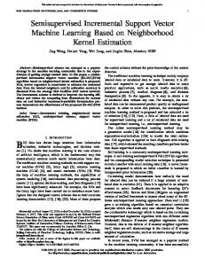
Each simulation is repeated 1000 times and the average RMSEs are reported. Figure 1 shows the RMSEs under Model 1 when the sample size of unlabeled data m is fixed as 30 and the sample size of labeled data n = 10, 30, 50, 100, 200, 300, 500, 800, 1000 and 1500. As n increases, the RMSEs of all methods decrease as expected. More importantly, the RMSE increases

11

as λ increases. In particular, the hard criterion always outperforms the soft criterion, which is consistent with our theoretical results. Figure 2 shows the RMSEs under Model 1 when n is fixed as 100 and m = 30, 60, 100, 300, 500 and 1000. As before, the RMSE always increases as λ increases. Moreover, the RMSEs of all methods increase as m increases, which suggests that the hard criterion may not be consistent when m grows faster than n. For the non-linear logit function, Figure 3 and 4 show the same patterns as in Figure 1 and 2, respectively, which also support our theoretical results.

5

Summary

In this article, we proved the consistency of graph-based semi-supervised learning when the tuning parameter of the graph Laplacian is zero (the hard criterion) and showed that the method can be inconsistent when the tuning parameter is nonzero (the soft criterion). Moreover, the numerical studies also suggest that the hard criterion outperforms the soft criterion in terms of the RMSE. These results provide a better understanding about the statistical properties of graph-based semisupervised learning. Of course, the accuracy of prediction can be measured by other indicators such as the area under the receiver operating characteristic curve (AUC). The hard criterion may not always be the best choice in term of these indicators. Further theoretical properties such as rank consistency will be explored in future research. Moreover, we would also like to investigate the behavior of these methods when the unlabeled data grow faster than the label data.

12

0.25

AVG RMSE

0.2

0.15

λ=0 λ=0.01 λ=0.1 λ=5

0.1

0

500

1000

1500

Values of n

Figure 1: Average RMSEs when m = 30 under Model 1

0.2

0.19

AVG RMSE

0.18

0.17

0.16

0.15 λ=0 λ=0.01 λ=0.1 λ=5

0.14 0

100

200

300

400

500

600

700

800

900

1000

Values of m

Figure 2: Average RMSEs when n = 100 under Model 1

13

0.24 0.22 0.2 0.18

AVG RMSE

0.16 0.14

0.12

0.1 λ=0 λ=0.01 λ=0.1 λ=5

0.08 0

500

1000

1500

Values of n

Figure 3: Average RMSEs when m = 30 under Model 2 0.24 0.23 0.22 0.21

AVG RMSE

0.2 0.19 0.18 0.17 0.16 λ=0 λ=0.01 λ=0.1 λ=5

0.15 0.14

0

100

200

300

400

500

600

700

800

900

1000

Values of m

Figure 4: Average RMSEs when n = 100 under Model 2

References [1] S. Basu, A. Banerjee, and R. J. Mooney. Semi-supervised clustering by seeding. In Proceedings of the International Conference on Machine Learning, pages 19–26, 2002. [2] M. Belkin, I. Matveeva, and P. Niyogi. Regularization and semi-supervised learning on large graphs. In Proceedings of the Seventeenth Annual Conference on Computational Learning Theory, pages 624–638, Banff, Canada, 2004.

14

[3] M. Belkin, P. Niyogi, and S. Sindhwani. Manifold Regularization: A geometric framework for learning from labeled and unlabeled examples. JMLR, 7:2399–2434, 2006. [4] T. De Bie and N. Cristianini. Convex methods for transduction. In Advances in Neural Information Processing Systems, 16:73–80, 2004. [5] O. Bosquet, O. Chapelle, and M. Hein. Measure based regularization. NIPS, 16, 2004. [6] Zongwu Cai. Weighted Nadaraya Watson regression estimation. Statistics & Probability Letters, 51:307–318, 2001. [7] O. Chapelle, B. Sch¨ olkopf, and A. Zien. Semi-supervised Learning. The MIT Press, 2006. [8] Olivier Delalleau, Yoshua Bengio, and Nicolas Le Roux. Efficient non-parametric function induction in semi-supervised learning. In Artificial Intelligence and Statistics, 2005. [9] Luc. P. Devroye. The uniform convergence of the Nadaraya-Watson regression function estimate. The Canadian Journal of Statistics, 6:179–191, 1978. [10] Luc. P. Devroye and T. J. Wagner. Distribution-free consistency results in nonparametric discrimination and regression function estimation. Annals of Statistics, 8(2):231–239, 1980. [11] M. Hein. Uniform convergence of adaptive graph-based regularization. COLT: Learning Theory, pages 50–64, 2006. [12] M.D. Intriligator and Z. Griliches. Handbook of Econometrics, volume 1. North-Holland Publishing Company, 1988. [13] Rosie Jones. Learning to extract entitles from labeled and unlabeled text. PhD Thesis, 2005. [14] John Lafferty and Larry Wasserman. Statistical analysis of semi-supervised regression. NIPS, 20, 2008. [15] E. A. Nadaraya. On estimating regression. Theor. Probability Appl, 9:141–142, 1964. [16] Boaz Nadler, Nathan Srebro, and Xueyuan Zhou. Semi-supervised learning with the Graph Laplacian: The limit of infinite unlabelled data. NIPS, 2009. [17] M. E. J. Newman. Networks: An introduction. Oxford University Press, 2010. [18] Joel Ratsaby and Santosh S. Venkatesh. Learning from a mixture of labeled and unlabeled examples with parametric side information. In Proceedings of COLT ’95 Proceedings of the eighth annual conference on Computational learning theory, pages 412–417, 1995. [19] Chuck Rosenberg, Martial Hebert, and Henry Schneiderman. Semi-supervised self-training of object detection models. In Proceedings of Seventh IEEE Workshop on Applications of Computer Vision, 2005. [20] V. Vapnik. Statistical Learning Theory. Wiley, New York, 1998. [21] G. S. Watson. Smooth regression analysis. Sankhy¯ a, Series A, 26:359–372, 1964. [22] D. Werner. Functional Analysis (in German). Springer Verlag, 2005.

15

[23] Y. Zhang, M. Brady, and S. Smith. Hidden markov random field model and segmentation of brain mr images. IEEE Transactions on Medical Imaging, 20(1):45–57, 2001. [24] D. Zhou, O. Bousquet, T. N. Lal, J. Weston, and B. Sch¨olkopf. Learning with local and global consistency. in S. Thrun, L. Saul, and B. Sch¨olkopf, editors. MIT Press, Cambridge, MA, 2004. [25] X. Zhu, Zoubin Ghahramani., and John Lafferty. Semi-supervised learning using Gaussian Fields and Harmonic Functions. ICML, (118), 2003. [26] X. Zhu and Andrew B. Goldberg. Introduction to Semi-supervised Learning. Morgan & Claypool Publishers, 2009.

16