On convex regression estimators Néstor Aguilera*
Liliana Forzani*
Pedro Morin*
arXiv:1006.2859v1 [math.ST] 14 Jun 2010
June 16, 2010
Abstract A new nonparametric estimator of a convex regression function in any dimension is proposed and its convergence properties are studied. We start by using any estimator of the regression function and we convexify it by taking the convex envelope of a sample of the approximation obtained. We prove that the uniform rate of convergence of the estimator is maintained after the convexification is applied. The finite sample properties of the new estimator are investigated by means of a simulation study and the application of the new method is demonstrated in examples.
Keywords: approximation, convex regression, convexity, data-smoothing, nonparametric regression
1
Introduction
In the nonparametric regression model 𝑌𝑛 = 𝑓 (𝑋𝑛 ) + 𝑒𝑛 ,
𝑛 = 1, 2, . . . ,
(1)
where 𝑌𝑛 ∈ R, 𝑋𝑛 ∈ R𝑑 and 𝑒𝑛 is an error term, it is not uncommon to have strong presumptions on properties of 𝑓 —such as monotonicity, convexity or concavity—which should be taken into account. Typical examples appear in economics (indirect utility, production or cost functions), medicine (dosage-response experiments) and biology (growth curves). A much studied case is the instance of a monotone regression function for 𝑑 = 1, estimated by using least squares (see, e.g., Brunk, 1955; Mukerjee, 1988, and Barlow et al., 1972 or Robertson et al., 1988 for a summary of this work). For convex (concave) regression Hildreth (1954) proposed to use convex least square estimates, and Hanson & Pledger (1976) proved their consistency. Algorithms for computing these estimates were developed by Wu (1982) and Fraser & Massam (1989), and the rate of convergence was derived by Mammen (1991). Later Groeneboom et al. (2001) derived the asymptotic distribution of the estimator at a fixed point of positive curvature. In all of these works the estimates hold pointwise. Still in one dimension, one can avoid the complications of least squares techniques and use more conventional smoothing methods when 𝑓 is convex (or * Consejo Nacional de Investigaciones Científicas y Técnicas, and Universidad Nacional del Litoral, Argentina
concave), as shown by Birke & Dette (2007). Using the fact that a differentiable function is convex (concave) if the derivative is increasing (decreasing), they propose to first smooth the data using any constrained nonparametric estimate (kernel type, local polynomial, series or spline estimator), then compute the derivative of the smooth function thus obtained, which is isotonized and finally integrated to recover a convex estimation. As mentioned above, the isotonization of a function is something that has already been mastered in the non-parametric literature, and using those results the rates of convergence obtained by them are the usual in non-parametric regression. Unfortunately this technique can only be used in one dimension and with smooth convex functions and cannot be extended to higher dimensions, since there is no such simple characterization of convexity in R𝑑 for 𝑑 > 1. As far as we know, little has been done in higher dimensions. Siem et al. (2005) (see also Hoffmann et al., 2006) present a multivariate data smoothing method using a linear program (for the ℓ1 and ℓ∞ norms) or quadratic program (for the ℓ2 norm). Shih et al. (2006) develop an approximation method based on multivariate adaptive regression splines (MARS). But none of these articles present convergence results. We propose here a simple and fast method that can be used in any dimension and applied to any convex function, even if not too smooth. Like Birke and Dette, we start by using any approximating scheme on the data, but then we use a convexification step, consisting in taking the convex envelope of the approximating function just obtained. This last step can be done very quickly by current software such as QHULL (Barber et al., 1996), and the uniform rate of convergence of the approximation technique is maintained after the convexification is applied. More precisely, we obtain uniform error estimates, and the rate of convergence of the convex estimator is the same as that of the original estimator, thereby showing that the convexification step adds basically no further errors to the estimating step. The paper is organized as follows. In Section 2 we briefly review fundamental smoothing techniques. In Section 3 we show theoretical results on the convexification step, and how the error estimates for the convex estimate are derived from the smoothing step. Finally, in Section 4 we apply these techniques to approximate several problems in dimensions 𝑑 = 1 and 𝑑 = 2.
2
The smoothing step: review of the literature
As we have already pointed out, our method of convexification inherits the 𝐿∞ rate of convergence from whichever smoothing process is chosen for the model (1). We think it is appropriate, then, to briefly review rates of convergence in 𝐿∞ norm for some of the possible choices for such a process when no monotonicity or convexity assumptions are made on 𝑓 . Most of the approximation techniques with known rates of convergence are of the so called smoothing type, where a variable kernel is used, and we will focus our attention on these. It should be noted that since there are many different schools and people involved, here we can give only partial references, leaving out several meaningful results available in the literature.
2
Perhaps the first ones to consider these problems were Devroye (1978) and Schuster & Yakowitz (1979). Devroye considered the Nadaraya-Watson regression estimator and proved the uniform convergence (without rates) for independent data, with fixed or random predictors belonging to R𝑑 , whereas Schuster and Yakowitz considered more general kernels in one dimension, establishing orders of convergence in probability. Later these results were extended by several authors, among them Bierens (1983) and Collomb (1984). They extended the result to non-independent data and Collomb was the first to give strong rates for uniform convergence. Further results on uniform convergence rates for different settings such as robust estimation and other kind of non-independent data were given by Collomb & Härdle (1986), Roussas (1990), Boente & Fraiman (1991), Truong & Stone (1992) and Tran (1993). Extensions to spline estimators were given by Eggermont & LaRiccia (2006), and to uniform choice of bandwidth by Einmahl & Mason (2005, 2000), Dony (2008), Dony & Einmahl (2006), Dony & Mason (2008), and Dony et al. (2006) (see also the references therein). The asymptotic distribution of the maximal deviation between a non-parametric regression estimator and the true regression was first considered by Johnston (1982), extending to the regression context the results by Bickel & Rosenblatt (1973) and Rosenblatt (1976) on density estimation. For the case 𝑑 = 1 and random predictors, Johnston showed—under some regularity assumptions— the 𝐿∞ asymptotic distribution of the kernel regression estimator, which allowed him to give uniform confidence intervals for the regression estimator. This result was extended by Konakov & Piterbarg (1984) to other kernel estimators and by Härdle (1989) to general estimators defined implicitly, as for example 𝑀 -smoothers and local polynomial estimators. As far as we know these results were not extended to higher dimensions or non-independent data.
3
A convex estimator and its convergence
Let us assume that the variables 𝑋𝑛 in the model (1) take values on a bounded closed convex set 𝑄 ⊂ R𝑑 , and that 𝑓 ∈ C , where C is the set of (finite real valued) convex functions defined on 𝑄. 𝑄 need not be polyhedral, but assuming its boundary is smooth except for a finite set of “corners”, in practice we may approximate it by a polyhedron. Thus, from now on, for simplicity we will assume that 𝑄 is a polyhedron, and therefore it is the convex hull of its finite set of vertices. In particular, we assume that 𝑄 is compact. Let us assume that 𝑓𝑛 is an estimator of 𝑓 , defined in all of 𝑄. To fix ideas, we may think that 𝑓𝑛 is obtained by considering the points (𝑋𝑖 , 𝑌𝑖 ), 𝑖 = 1, . . . , 𝑛, by some procedure such as smoothing. Our purpose is to derive from 𝑓𝑛 another estimator which is also convex. To do so, we consider a finite set ℳ𝑛 ⊂ 𝑄 such that the convex hull of ℳ𝑛 is 𝑄. The number of points in ℳ𝑛 need not be 𝑛 and the points in ℳ𝑛 might be completely unrelated to {𝑋𝑖 : 𝑖 ∈ N}. We now let L𝑛 be the set of “convex functions below 𝑓𝑛 on ℳ𝑛 ”, {︀ }︀ L𝑛 = 𝜓 ∈ C : 𝜓(𝑥) ≤ 𝑓𝑛 (𝑥) for all 𝑥 ∈ ℳ𝑛 , and define the convex estimator 𝑓𝑛𝑐 , associated with the estimator 𝑓𝑛 and the
3
set ℳ𝑛 by
𝑓𝑛𝑐 = sup {𝜓 : 𝜓 ∈ L𝑛 }.
(2)
Since ℳ𝑛 contains all the vertices of 𝑄, it is easy to see that 𝑓𝑛𝑐 is well defined on 𝑄 and that 𝑓𝑛𝑐 ∈ C . Furthermore, 𝑓𝑛𝑐 is piecewise linear, determined by the maximum of hyperplanes. In particular: Lemma 1. 𝑓𝑛𝑐 ∈ L𝑛 . As 𝑓𝑛𝑐 is the “lower part” of the convex hull of the set {(𝑥, 𝑓𝑛 (𝑥)) : 𝑥 ∈ ℳ𝑛 }, we may take advantage of any of a number of algorithms for finding convex hulls in R𝑑 . For instance, QHULL (Barber et al., 1996) finds the convex hull of a finite set of points in any number of dimensions, and is really fast for dimensions 𝑑 ≤ 4. We are led to the following procedure for constructing a convex estimator 𝑓𝑛𝑐 of 𝑓 : Procedure 2. Given 𝑋𝑖 and 𝑌𝑖 (𝑖 = 1, 2, . . . ): Step 1. (Smoothing) Construct an estimator 𝑓𝑛 of 𝑓 , for instance through a smoothing procedure using the values 𝑋𝑖 and 𝑌𝑖 for 𝑖 = 1, . . . , 𝑛. Step 2. (Grid of points) Choose 𝛿𝑛 > 0 and ℳ𝑛 ⊂ 𝑄 so that any 𝑥 ∈ 𝑄 is the convex combination of points in ℳ𝑛 whose distance to 𝑥 is not more than 𝛿𝑛 . Step 3. (Convexification) Construct 𝑓𝑛𝑐 as in (2), for instance by using a convex hull procedure such as QHULL. In Figure 1 we represent the steps of the procedure with an example: in (a) we show the data and the resulting estimator 𝑓𝑛 ; in (b) we show the estimator and its values at the points of ℳ𝑛 ; in (c) we show the convex estimator 𝑓𝑛𝑐 obtained from the values of 𝑓𝑛 at ℳ𝑛 ; and in (d) we compare the original data and the convex estimator obtained. We now show that if in the Procedure 2, 𝑓𝑛 is a good approximation of 𝑓 , then 𝑓𝑛𝑐 is a good approximation of 𝑓 provided it satisfies: H-1. 𝑓 is a continuous convex function defined on 𝑄, with ‖𝑓 ‖Lip = 𝐿 < ∞, where ‖𝑓 ‖Lip = sup{|𝑓 (𝑥) − 𝑓 (𝑦)|/|𝑥 − 𝑦| : 𝑥, 𝑦 ∈ 𝑄, 𝑥 ̸= 𝑦}. and |𝑥−𝑦| denotes the (Euclidean) distance between 𝑥 and 𝑦 in R𝑑 . (Recall that convex functions on 𝑄 are locally Lipschitz, but here we require that 𝑓 be uniformly Lipschitz in all of 𝑄.) Theorem 3. Suppose 𝑓 satisfies H-1 and let 𝑓𝑛 , 𝛿𝑛 , ℳ𝑛 and 𝑓𝑛𝑐 be as in Procedure 2, with sup {|𝑓𝑛 (𝑥) − 𝑓 (𝑥)| : 𝑥 ∈ ℳ𝑛 } ≤ 𝜀𝑛 . Then, −𝜀𝑛 ≤ 𝑓𝑛𝑐 (𝑥) − 𝑓 (𝑥) ≤ 𝜀𝑛 + 𝐿𝛿𝑛
4
for all 𝑥 ∈ 𝑄.
(3)
1.2
1.2
1
1
0.8
0.8
0.6
0.6
0.4
0.4
0.2
0.2
0
0
−0.2
−0.2
0
0.1
0.2
0.3
0.4
0.5
0.6
0.7
0.8
0.9
1
0
1.2
1.2
1
1
0.8
0.8
0.6
0.6
0.4
0.4
0.2
0.2
0
0
−0.2
−0.2
0
0.1
0.2
0.3
0.4
0.5
(c) Convex estimator
0.6
𝑓𝑛𝑐
0.7
0.8
0.1
0.2
0.3
0.4
0.5
0.6
0.7
0.8
0.9
1
(b) Estimator 𝑓𝑛 and its values on ℳ𝑛
(a) Data and estimator 𝑓𝑛
0.9
1
0
from 𝑓𝑛 on ℳ𝑛
0.1
0.2
0.3
0.4
0.5
0.6
0.7
0.8
(d) Data and convex estimator
Figure 1: Steps in constructing a convex estimator
5
0.9
𝑓𝑛𝑐
1
Proof. Since 𝑓 is convex and 𝜀𝑛 is a constant, the function 𝑓 − 𝜀𝑛 is convex. Moreover, 𝑓 (𝑥) − 𝜀𝑛 ≤ 𝑓𝑛 (𝑥) for all 𝑥 ∈ ℳ𝑛 implies that 𝑓 − 𝜀𝑛 ∈ L𝑛 , and by the definition of 𝑓𝑛𝑐 in (2), 𝑓 (𝑥) − 𝜀𝑛 ≤ 𝑓𝑛𝑐 (𝑥) for all 𝑥 ∈ 𝑄, proving one inequality. For the other inequality, consider 𝑥 ∈ 𝑄, and let 𝑥𝑘 ∈ ℳ𝑛 and 𝜆𝑘 ≥ 0, 𝑘 = 1, . . . , 𝑑 + 1, be such that ∑︁ ∑︁ 𝜆𝑘 𝑥𝑘 = 𝑥, 𝜆𝑘 = 1, and |𝑥 − 𝑥𝑘 | ≤ 𝛿𝑛 for 𝑘 = 1, . . . , 𝑑 + 1. 𝑘
𝑘
Then, 𝑓𝑛𝑐 (𝑥) ≤
∑︁
≤
∑︁
𝜆𝑘 𝑓𝑛𝑐 (𝑥𝑘 )
since 𝑓𝑛𝑐 ∈ C ,
𝜆𝑘 𝑓𝑛 (𝑥𝑘 )
by Lemma 1,
𝜆𝑘 (𝑓 (𝑥𝑘 ) + 𝜀𝑛 )
by (3),
𝑘
𝑘
∑︁
≤
𝑘
(︂∑︁
=
)︂ 𝜆𝑘 𝑓 (𝑥𝑘 ) + 𝜀𝑛
since
∑︁
𝑘
𝜆𝑘 = 1.
𝑘
Now, ‖𝑓 ‖Lip = 𝐿 and |𝑥𝑘 − 𝑥| < 𝛿𝑛 , and therefore 𝑓 (𝑥𝑘 ) ≤ 𝑓 (𝑥) + 𝐿𝛿𝑛 . ∑︀ Hence, since 𝜆𝑘 ≥ 0 and using again that 𝑘 𝜆𝑘 = 1, we conclude )︂ (︂∑︁ 𝑐 𝑓𝑛 (𝑥) ≤ 𝜆𝑘 (𝑓 (𝑥) + 𝐿𝛿𝑛 ) + 𝜀𝑛 = 𝑓 (𝑥) + 𝐿𝛿𝑛 + 𝜀𝑛 , 𝑘
and the result follows. Remark. In the proof we have not used the finiteness of ℳ𝑛 , and only the values of 𝑓𝑛 on ℳ𝑛 are used. Noticing that given 𝛿𝑛 > 0 we may construct a finite set ℳ𝑛 with the property that any 𝑥 ∈ 𝑄 is a convex combination of points in ℳ𝑛 whose distance to 𝑥 is no more than 𝛿𝑛 , we have: Corollary 4. If 𝑓 satisfies H-1, given an estimator 𝑓𝑛 of 𝑓 and 𝛿𝑛 > 0, we may find ℳ𝑛 and define 𝑓𝑛𝑐 according to Procedure 2, so that ‖𝑓𝑛𝑐 − 𝑓 ‖∞ ≤ ‖𝑓𝑛 − 𝑓 ‖∞ + 𝐿𝛿𝑛 . Remark. In the extreme case where 𝑓𝑛 = 𝑓 for all 𝑛, we have ‖𝑓𝑛 − 𝑓 ‖∞ = 0, but ‖𝑓𝑛𝑐 − 𝑓 ‖∞ > 0 in general (for instance, if ℳ𝑛 is finite and 𝑓 is not piecewise linear). Corollary 4 tells us that the convex estimator 𝑓𝑛𝑐 obtained through the Procedure 2 inherits the approximation properties of the original estimator 𝑓𝑛 ,
6
and the rate of convergence is preserved or even bettered provided 𝛿𝑛 is small enough. To illustrate this behavior, let us consider the following well-known types of convergence of a sequence of nonnegative random variables (𝑅𝑛 )𝑛 to 0, where (𝑟𝑛 )𝑛 is a bounded sequence of positive numbers (possibly converging to 0), and we have denoted by P the underlying probability measure: T-1. For every 𝜀 > 0 there exists 𝑀 > 0 such that sup𝑛 P(𝑅𝑛 > 𝑀 𝑟𝑛 ) < 𝜀. T-2. lim𝑛→∞ P(𝑅𝑛 > 𝜀𝑟𝑛 ) = 0 for every 𝜀 > 0. T-3. 𝑅𝑛 = 𝑂(𝑟𝑛 ) or 𝑅𝑛 = 𝑜(𝑟𝑛 ) a.s. ∑︀∞ T-4. For every 𝜀 > 0, 𝑛=1 P(𝑅𝑛 > 𝜀𝑟𝑛 ) < ∞. It is easy to see that: Theorem 5. If any of T-1 through T-4 holds for 𝑅𝑛 = ‖𝑓𝑛 − 𝑓 ‖∞ , then it also holds for 𝑅𝑛 = ‖𝑓𝑛𝑐 − 𝑓 ‖∞ , provided 𝑓 satisfies H-1 and 𝑓𝑛𝑐 is constructed as in Corollary 4 with 𝛿𝑛 = 𝑜(𝑟𝑛 ). For example, Tran (1993) shows: Theorem 6. For 𝑗 = 1, 2, . . . , let {(𝑋𝑗 , 𝑌𝑗 )}𝑗 be a strictly stationary sequence of random variables, where the 𝑋𝑗 and the 𝑌𝑗 are R𝑑 -valued and R-valued, respectively. Suppose 𝑓 (𝑥) = E(𝑌 | 𝑋 = 𝑥) is estimated by 𝑓𝑛 (𝑥) =
∑︁ 1 𝑌𝑖 #(𝐼𝑛 (𝑥))
for 𝑥 ∈ 𝑄,
𝑖∈𝐼𝑛 (𝑥)
1/(𝑑+2)
where 𝐼𝑛 (𝑥) = {𝑖 : 1 ≤ 𝑖 ≤ 𝑛, |𝑋𝑖 − 𝑥| ≤ ℎ𝑛 }, and ℎ𝑛 ≈ (log(𝑛)/𝑛) . Then, under appropriate assumptions (including adequate regularity conditions), ‖𝑓𝑛 − 𝑓 ‖𝐿∞ (𝑄) = 𝑂(ℎ𝑛 ) a.s. Tran’s result gives a T-3 type of convergence, and therefore (by Theorem 5) we have that under the same assumptions, ‖𝑓𝑛𝑐 − 𝑓 ‖𝐿∞ (𝑄) = 𝑂(ℎ𝑛 ) a.s., provided we take 𝛿𝑛 = 𝑜(ℎ𝑛 ) in Corollary 4. More elaborate types of convergence include exact asymptotic behavior. A very simple model might be, assuming 𝑋𝑛 uniformly distributed on 𝑄: T-5. There exist a sequence (𝑑𝑛 )𝑛 converging to 0, and a random variable 𝑅 such that P(𝑟𝑛−1 (𝑅𝑛 − 𝑑𝑛 ) ≤ 𝑡) → P(𝑅 ≤ 𝑡), for every 𝑡 ∈ R at which P(𝑅 ≤ 𝑡) is continuous. It is not possible in general to carry over this convergence from 𝑅𝑛 = ‖𝑓𝑛 − 𝑓 ‖∞ directly to 𝑅𝑛 = ‖𝑓𝑛𝑐 − 𝑓 ‖∞ , as in general ‖𝑓𝑛𝑐 − 𝑓 ‖∞ could be much smaller than ‖𝑓𝑛 − 𝑓 ‖∞ , and we cannot control ‖𝑓𝑛 − 𝑓 ‖∞ solely in terms of
7
‖𝑓𝑛𝑐 − 𝑓 ‖∞ and ‖𝑓 ‖Lip . Needless to say, by enlargening 𝑟𝑛 we may transform a T-5 type into, say, a T-2 type of convergence. Besides the interest in itself, the convergence of type T-5 allows us to find uniform confidence bands for the regression curve, which is a practical concern. More precisely, if T-5 is verified, for any 𝛼, 0 < 𝛼 < 1, we may find optimal (or near optimal) 𝑠 so that P(𝑅𝑛 ≤ 𝑠) ≥ 1 − 𝛼. (4) If this inequality holds for 𝑅𝑛 = ‖𝑓𝑛 − 𝑓 ‖∞ and assuming 𝑓𝑛𝑐 is constructed as in Corollary 4 with 𝛿𝑛 = 𝑜(1) for all 𝑛, then (4) is valid for 𝑅𝑛 = ‖𝑓𝑛𝑐 − 𝑓 ‖∞ , albeit not with optimal 𝑠. In other words, Corollary 4 allows us to convert a uniform confidence band for 𝑓𝑛 of the form (4) into a (slightly different) uniform confidence band for 𝑓𝑛𝑐 . For instance, Johnston (1982, Theorem 2.1) shows: Theorem 7. Let (𝑋1 , 𝑌1 ), . . . , (𝑋𝑛 , 𝑌𝑛 ) be a random sample from a bivariate population, with 𝑋 uniformly distributed in 𝑄 = [0, 1], and consider the following estimator of 𝑓 (𝑥) = E(𝑌 | 𝑋 = 𝑥), 𝑓𝑛 (𝑥) =
𝑛 1 ∑︁ 𝑌𝑖 𝐾((𝑥 − 𝑋𝑖 )/ℎ𝑛 ), 𝑛ℎ𝑛 𝑖=1
(5)
where ℎ𝑛 ≈ 𝑛−𝛿 for some 𝛿, 1/5 < 𝛿 < 1/3, and 𝐾 is a piecewise smooth density function with support in [−𝐴, 𝐴], 𝐴 > 1. Then, under appropriate regularity assumptions we have (︂ [︂ ]︂ )︂ (︀ )︀ P (2𝛿 log 𝑛)1/2 sup 𝑟𝑛−1 (𝑥) 𝑓𝑛 (𝑥) − 𝑓 (𝑥) − 𝑑𝑛 < 𝑡 → 𝑒−2 exp (−𝑡) , 0≤𝑥≤1
where
∫︀ 𝑟𝑛2 (𝑥)
=
𝐾 2 (𝑢) 𝑑𝑢 × E(𝑌 2 | 𝑋 = 𝑥) 𝑛ℎ𝑛
(6)
(︀ )︀ and 𝑑𝑛 = 𝑂 (2𝛿 log 𝑛)1/2 . Confidence bands follow immediately (Johnston, 1982, Corollary 3.1): Corollary 8. Assuming Theorem 7 holds, an approximate (1 − 𝛼) × 100% confidence band is (︀ )︀ 𝑓𝑛 (𝑥) ± 𝑟𝑛 𝑑𝑛 + 𝑐(𝛼)(2𝛿 log 𝑛)−1/2 , where 𝑐(𝛼) = log 2−log | log(1−𝛼)| (for practical applications, one would estimate E(𝑌 2 | 𝑋 = 𝑥) in (6)). Theorem 7 and its corollary are still valid if instead of (5), 𝑓𝑛 is a 𝑀 −smoother estimator defined as a solution of 0=
𝑛 1 ∑︁ 𝜓(𝑌𝑖 − 𝑓𝑛 ) 𝐾((𝑥 − 𝑋𝑖 )/ℎ𝑛 ), 𝑛ℎ𝑛 𝑖=1
with 𝜓 a bounded monotone, antisymmetric real function (Härdle, 1989).
8
As a final remark, let us point out that we have only used that 𝑓𝑛 approximates the Lipschitz convex function 𝑓 , independently of whether 𝑓𝑛 has been obtained through a smoothing procedure or any other approximation method.
4
Numerical results
In this section we report on some practical aspects of our algorithm and present some simulations and examples showing its performance.
4.1
Implementation
We implemented our algorithm using MATLAB. The smoothing step was done with local polynomials of degree 1 with Gauss’s kernel, and for the convexification we used MATLAB’s functions convhull (dimension 1) and convhulln (higher dimensions), which are based upon the QHULL algorithm described in Barber et al. (1996). The bandwidth was chosen using cross-validation for the local-polynomial fitting at the data points. In the examples shown below, once the optimal bandwidth was chosen, the local-polynomial fitting function was computed at the same data points which were set a priori as design. Whenever the data points were not a priori designed, the local-polynomial fit was evaluated on a uniform grid having approximately the same number of points.
4.2
One dimensional simulations
In this section we briefly illustrate the finite sample properties of the convex estimate of the regression function by means of a simulation study. For this purpose we considered the same three examples presented in Birke & Dette (2007), namely, 𝑓1 (𝑥) = 𝑒3(𝑥−1) , (︂ )︂2 16 1 𝑓2 (𝑥) = 𝑥− , 9 4 ⎧ ⎪ ⎨−4𝑥 + 1 if 0 ≤ 𝑥 ≤ 1/4, 𝑓3 (𝑥) = 0 if 1/4 < 𝑥 < 3/4, ⎪ ⎩ 4𝑥 − 3 if 3/4 ≤ 𝑥, and 𝑄 = [0, 1]. Notice that even though the third function is just Lipschitz, all these functions satisfy the assumption H-1. As in Birke & Dette (2007), we ran some simulations with 𝑛 = 100 uniformly distributed design points for the explanatory variables and added a normal noise with standard deviation 𝜎 = 0.1 to the response variable. In Figure 2 we display for each regression function five typical estimates obtained from different simulation runs observing a typical performance. The estimates for the two smooth functions 𝑓1 and 𝑓2 are comparable to the regressions obtained in Birke & Dette (2007), but our estimates of the nonsmooth regression function 𝑓3 exhibit a much closer fit. This is an advantage of our method,
9
1 1
1
0.8
0.8
0.6
0.6
0.9 0.8 0.7 0.6 0.5 0.4
0.4
0.4
0.3 0.2
0.2
0.2
0.1 0
0
0 0
0.1
0.2
0.3
0.4
0.5
0.6
0.7
0.8
0.9
1
0
0.1
0.2
0.3
0.4
0.5
0.6
0.7
0.8
0.9
1
0
0.1
0.2
0.3
0.4
0.5
0.6
0.7
0.8
0.9
1
Figure 2: Regression functions 𝑓1 (left), 𝑓2 (middle), 𝑓3 (right), and their estimates. Result of 5 simulations for each regression function, with sample size 𝑛 = 100 and normal errors with 𝜎 = 0.1. The estimates are very reasonable, even for 𝑓3 , which is just Lipschitz, and not 𝐶 1 .
which does not approximate the derivative of the regression function, and thus it demands less smoothness and approximates better non differentiable functions. In the second part of this simulation study we investigated the mean square error, bias and variance of our convex estimate. For this we considered again the three regression functions in 𝑓1 , 𝑓2 , 𝑓3 and computed—with 2000 simulation runs—the curves for the mean square error, squared bias and variance. The results shown in Figure 3 look very much alike those in Birke & Dette (2007), except for the ones related to 𝑓3 , where our estimator seems to be better. In this figure the mean square error, bias and variance of the estimator by local linear polynomials are represented by the dashed lines, while those quantities related to our convex estimator are represented by the solid lines. Finally, in Figure 4 we show approximate 95% confidence bands for one estimate to each of the previous regression functions. We ran a simulation with 100 uniformly distributed design points for the explanatory variables and added a normal noise with 𝜎 = 0.1 to the response variable. In order to use the existing results on the width of the confidence bands from Johnston (1982, Corollary 3.1) (see also Theorem 7 and its corollary), the smoothing step was done with the formula 𝑛 1 ∑︁ 𝑓𝑛 (𝑥) = 𝐾((𝑥 − 𝑋𝑖 )/ℎ𝑛 ), 𝑛ℎ𝑛 𝑗=1 where 𝐾(𝑥) = 34 (1 − 𝑥2 )+ is Epanechnikov’s Kernel. This regression formula has bad approximation properties at the endpoints of the interval, which explains the mild misfit observed there. The width of the band was 0.1392, 0.1382, 0.1628, for the estimate corresponding to 𝑓1 , 𝑓2 , and 𝑓3 , respectively.
4.3
Rabbits’ data
We studied an example considered in Dudzinski & Mykytowycz (1961), who analyzed the relationship between age and eye lens weight for rabbits in Australia. This relationship is expected to be guided by a concave function. In this study, the dry weight of the eye lens was measured (in milligrams) for 71 free-living wild rabbits of known age (measured in days). A detailed description of the experiment and the data can be found in http://www.statsci.org/data/oz/rabbit.html. The data was analyzed by Ratkowsky (1983) using a parametric nonlinear growth
10
Bias2
Var
MSE
−4
x 10
−3
x 10 2.5
−3
x 10
4 2.5
2
3
2
1.5 1.5
2 1
1
1
0.5
0.5
0
0
0.2
0.4
0.6
0.8
1
0
0
−3
0.2
0.4
0.6
0.8
1
0
−4
x 10
2.5
0
0.2
0.4
0.6
0.8
1
0.2
0.4
0.6
0.8
1
0.8
1
−3
x 10
x 10
2.5
2.5 2
2
2 1.5
1.5
1.5 1
1
1
0.5
0.5
0
0
0.2
0.4
0.6
0.8
1
0.5
0
0
0.2
0.4
0.6
0.8
1
0
0
−3
x 10 4
0.02
0.02
0.015
0.015
0.01
0.01
0.005
0.005
3.5 3 2.5 2 1.5 1 0.5 0
0
0.2
0.4
0.6
0.8
1
0
0
0.2
0.4
0.6
0.8
1
0
0
0.2
0.4
0.6
Figure 3: Variance (left), squared Bias (middle) and Mean Square Error (right) of our convex estimate (solid line) and of the local linear estimate (dashed line). These indicators were obtained with 2000 simulation runs, for 𝑓1 (top), 𝑓2 (middle) and 𝑓3 (bottom), using 100 uniformly distributed design points for the explanatory variable, and normal error with 𝜎 = 0.1 for the observed variable. Only small differences between the local linear estimate and our convex estimate are observed. In some cases, our convex estimate is even better.
1.2
1.2
1
1
1
0.8
0.8
0.8
0.6
0.6
0.6
0.4
0.4
0.4
0.2
0.2
0.2
0 −0.2
0
0.2
0.4
0.6
0.8
1
1.2
0
0
−0.2
−0.2 0
0.2
0.4
0.6
0.8
1
0
0.2
0.4
0.6
0.8
1
Figure 4: Approximate 95% confidence bands. In each plot we show the exact regression function, the estimate, the 95% confidence bands, and the data points for 𝑁 = 100 design points, and normal error with 𝜎 = 0.1. The bands have width 0.1392, 0.1382, and 0.1628 for 𝑓1 (left), 𝑓2 (middle), 𝑓3 (right), which were computed with the formula provided in Corollary 8.
11
250
250
200
200
150
150
100
100
50
0
50
convex regression smoothed data data 0
200
400
600
0
800
convex regression smoothed data data 0
200
400
600
800
Figure 5: Convex regression of the rabbits’ data. Dry weight of the eye lens (milligrams) versus age (days). Plot of the local polynomial smoothing (dashed blue), the convex estimate (solid red), and data points (magenta). The smoothing step is based on local polynomials of degree 1 (left) and degree 2 (right). The fit obtained is really excellent, with no essential difference between degree 1 and 2. model, and by Birke & Dette (2007) with their non-parametric convex regression method. We used our method to obtain the concave regression, with the smoothing step performed with local polynomials of degree 1 and 2, and report the findings in Figure 5. In both cases, the bandwidth for the local polynomial smoothing was set using cross-validation, and the result of the smoothing step was evaluated at a uniform grid of 100 points. The convexification step yielded the estimated regression curves that can be observed in Figure 5 with an excellent fit to the data.
4.4
Two dimensional simulations
In this section we briefly illustrate the finite sample properties of the convex estimate of a regression function in two dimensions by means of a simulation study. For this purpose we considered the following convex regression function: {︀ }︀ 𝑓 (𝑥1 , 𝑥2 ) = max 2𝑥21 + 𝑥22 /2, 3𝑥1 + 𝑥2 , which is convex, and only Lipschitz. In Figure 6 we show the level curves of two estimated regression functions and the exact one in two simulations. We took uniform grids of 10 × 10, and 20 × 20 in each situation for the explanatory variable, and added normal error with 𝜎 = 0.1 to the value of 𝑓 (𝑥1 , 𝑥2 ) to emulate an observed variable. The level curves shown in the figure show a very good fit, even for a coarse grid of only 20 × 20 points. In the second part of this simulation study we investigated the mean square error, bias and variance of our convex estimate. For this we considered again the same two dimensional regression function 𝑓 and calculated by 2000 simulation runs the surfaces for the mean square error, squared bias and variance. The results depicted in Figure 7 show that the variance is concentrated on the boundary but is one order of magnitude smaller than the squared bias and the mean square error. These last two quantities are concentrated on the region of the domain where the regression function is not 𝐶 1 . 12
1
1
0.5
0.5
0
0
−0.5
−0.5
−1 −1
−0.5
0
0.5
1
−1 −1
−0.5
0
0.5
1
Figure 6: Level curves of two estimated regression functions (dashed red and magenta) and the exact one (solid blue) in two simulations with uniform design for the explanatory variables. One for a grid of 10 × 10 (left) points and another for a grid of 20 × 20 (right). The fit looks very good, even for a grid of only 20 × 20 points.
Bias2
Var
MSE
−3
x 10 5
0.05
0.05
4
0.04
0.04
3
0.03
0.03
2
0.02
0.02
1
0.01
0.01
0 1
0 1
0 −1 −1
−0.5
0
0.5
0 1
1 0 −1 −1
−0.5
0
0.5
1 0 −1 −1
−0.5
0
0.5
1
Figure 7: Variance (left), squared Bias (middle) and Mean Square Error (right) for the two dimensional simulation. These indicators were obtained with 2000 simulation runs, using 10 × 10 (left) and 20 × 20 uniformly distributed design points for the explanatory variable, and normal error with 𝜎 = 0.1 for the observed variable.
13
40 14
35
12
30
8
x2
y
10
25
6
20 4 2 10
15 20
30
40
15
5
10
x2
0
10 2
x1
4
6
x1
8
10
12
Figure 8: Pareto surface obtained as the convex regression of the data points (left). Contour curves of the convex graph (right) showing an excelent fit of the data (see also Figure 2 of Hoffmann et al., 2006).
4.5
Radiotherapy data
We studied a two dimensional example considered in Siem et al. (2005) (see also Hoffmann et al., 2006), who approximated the Pareto surface of a multiobjective optimization problem arising in the computation of the precise radiation dose. This Pareto surface is convex under certain conditions, and it should be computed from some Pareto points that can be measured from the patient. We obtained data from a patient of the Radboud University Nijmegen Medical Centre, in Nijmegen, the Netherlands. The data correspond to a multiobjective optimization problem with three objectives and contains 69 data points, which, due to measuring errors, are not convex. By using our method we are able to smooth the data, obtaining a convex Pareto surface defined as a maximum of planes. This surface is initially defined on the convex hull of the 𝑋 data, and we have extended it to a rectangular domain by considering the same maximum of planes. In Figure 8 we show the data points together with the convex regression surface (left), and the contours of the convex regression (right), showing an excelent fit of the data (see also Figure 2 in Hoffmann et al., 2006).
Acknowledgements We would like to thank A. Hoffmann and A. Siem for sharing with us the data of the Radboud University Nijhmegen Medical Centre, used in Section 4.5.
References Barber, C. B., Dobkin, D. P. & Huhdanpaa, H. (1996). The quickhull algorithm for convex hulls. ACM Trans. Math. Software 22, 469–483. Barlow, R. E., Bartholomew, D. J., Bremner, J. M. & Brunk, H. D. (1972). Statistical inference under order restrictions. The theory and application of isotonic regression. John Wiley & Sons, London-New York-Sydney. Wiley Series in Probability and Mathematical Statistics.
14
Bickel, P. J. & Rosenblatt, M. (1973). On some global measures of the deviations of density function estimates. Ann. Statist. 1, 1071–1095. Bierens, H. J. (1983). Uniform consistency of kernel estimators of a regression function under generalized conditions. J. Amer. Statist. Assoc. 78, 699–707. Birke, M. & Dette, H. (2007). Estimating a convex function in nonparametric regression. Scand. J. Statist. 34, 384–404. Boente, G. & Fraiman, R. (1991). Strong uniform convergence rates for some robust equivariant nonparametric regression estimates for mixing processes. International Statistical Review 59, 355–372. Brunk, H. D. (1955). Maximum likelihood estimates of monotone parameters. Ann. Math. Statist. 26, 607–616. Collomb, G. (1984). Prédiction non paramétrique: étude de l’erreur quadratique du prédictogramme. Statist. Anal. Données 9, 1–34. Collomb, G. & Härdle, W. (1986). Strong uniform convergence rates in robust nonparametric time series analysis and prediction: kernel regression estimation from dependent observations. Stochastic Process. Appl. 23, 77–89. Devroye, L. (1978). The uniform convergence of the Nadaraya-Watson regression function estimate. Canad. J. Statist. 6, 179–191. Dony, J. (2008). Nonparametric regression estimation. PhD in Mathematical sciences, Free University of Brussels. Dony, J. & Einmahl, U. (2006). Weighted uniform consistency of kernel density estimators with general bandwidth sequences. Electron. J. Probab. 11, no. 33, 844–859 (electronic). Dony, J., Einmahl, U. & Mason, D. M. (2006). Uniform in bandwidth consistency of local polynomial regression function estimators. Austr. J. Statist. 35, 105– 120. Dony, J. & Mason, D. M. (2008). Uniform in bandwidth consistency of conditional 𝑈 -statistics. Bernoulli 14, 1108–1133. Dudzinski, M. & Mykytowycz, R. (1961). The eye lens as an indicator of age in the wild rabbit in australia. CSIRO Wildlife Research 6, 156–159. Eggermont, P. P. B. & LaRiccia, V. N. (2006). Uniform error bounds for smoothing splines. In High dimensional probability, vol. 51 of IMS Lecture Notes Monogr. Ser. Inst. Math. Statist., Beachwood, OH, 220–237. Einmahl, U. & Mason, D. M. (2000). An empirical process approach to the uniform consistency of kernel-type function estimators. J. Theoret. Probab. 13, 1–37. Einmahl, U. & Mason, D. M. (2005). Uniform in bandwidth consistency of kernel-type function estimators. Ann. Statist. 33, 1380–1403.
15
Fraser, D. A. S. & Massam, H. (1989). A mixed primal-dual bases algorithm for regression under inequality constraints. Application to concave regression. Scand. J. Statist. 16, 65–74. Groeneboom, P., Jongbloed, G. & Wellner, J. A. (2001). Estimation of a convex function: characterizations and asymptotic theory. Ann. Statist. 29, 1653–1698. Hanson, D. L. & Pledger, G. (1976). Consistency in concave regression. Ann. Statist. 4, 1038–1050. Härdle, W. (1989). Asymptotic maximal deviation of 𝑀 -smoothers. J. Multivariate Anal. 29, 163–179. Hildreth, C. (1954). Point estimates of ordinates of concave functions. J. Amer. Statist. Assoc. 49, 598–619. Hoffmann, A. L., Siem, A. Y. D., den Hertog, D., Kaanders, J. & H., H. (2006). Derivative-free generation and interpolation of convex Pareto optimal IMRT plans. Physics in Medicine and Biology 51, 6349–6369. Johnston, G. J. (1982). Probabilities of maximal deviations for nonparametric regression function estimates. J. Multivariate Anal. 12, 402–414. Konakov, V. D. & Piterbarg, V. I. (1984). On the convergence rate of maximal deviation distribution for kernel regression estimates. J. Multivariate Anal. 15, 279–294. Mammen, E. (1991). Nonparametric regression under qualitative smoothness assumptions. Ann. Statist. 19, 741–759. Mukerjee, H. (1988). Monotone nonparameteric regression. Ann. Statist. 16, 741–750. Ratkowsky, D. (1983). Nonlinear regression modeling. Marcel Dekker Inc. Robertson, T., Wright, F. T. & Dykstra, R. L. (1988). Order restricted statistical inference. Wiley Series in Probability and Mathematical Statistics: Probability and Mathematical Statistics. John Wiley & Sons Ltd., Chichester. Rosenblatt, M. (1976). On the maximal deviation of 𝑘-dimensional density estimates. Ann. Probability 4, 1009–1015. Roussas, G. G. (1990). Nonparametric regression estimation under mixing conditions. Stochastic Process. Appl. 36, 107–116. Schuster, E. & Yakowitz, S. (1979). Contributions to the theory of nonparametric regression, with application to system identification. Ann. Statist. 7, 139–149. Shih, T. D., Chen, V. C. P. & Kim, S. B. (2006). Convex version of multivariate adaptive regression splines for optimization. Proceedings of the 2006 IE Research Conference (Orlando, FL) (preprint: http://students.uta.edu/ dt/dts5878/convexMARS.pdf).
16
Siem, A. Y. D., den Hertog, D. & L., H. A. (2005). Multivariate convex approximation and least-norm convex data-smoothing. CentER Discussion Paper 2005-73, 1–21. Tran, L. T. (1993). Nonparametric function estimation for time series by local average estimators. Ann. Statist. 21, 1040–1057. Truong, Y. K. & Stone, C. J. (1992). Nonparametric function estimation involving time series. Ann. Statist. 20, 77–97. Wu, C.-F. (1982). Some algorithms for concave and isotonic regression. In Optimization in statistics, vol. 19 of Stud. Management Sci. North-Holland, Amsterdam, 105–116.
Corresponding author: Liliana Forzani Address: IMAL, Güemes 3450, 3000 Santa Fe, Argentina e-mail:
[email protected]
17