500. As it is known from [9], these distribution of SVs leads to large saving in the ..... 500 x 500. 158.8 164.1. 140.6 143.3. Table 4.2. Pre-processing (PDGEQPF) ...
Proceedings of ALGORITMY 2009 pp. 449–458
ON DATA LAYOUT IN THE PARALLEL BLOCK-JACOBI SVD ALGORITHM WITH PRE–PROCESSING ∗ ˇ ˇ † , MARIAN ´ VAJTERSIC ˇ ‡ , AND LAURA GRIGORI§ MARTIN BECKA , GABRIEL OKSA Abstract. An efficient version of the parallel two-sided block-Jacobi algorithm for the singular value decomposition of an m × n matrix A includes the pre-processing step, which consists of the QR factorization of A with column pivoting followed by the optional LQ factorization of the Rfactor. Then the iterative two-sided block-Jacobi algorithm is applied in parallel to the R-factor (or L-factor). Having p processors, these iterations are efficiently computed with two block-columns stored in each processor; hence the blocking factor is ℓ = 2p and the process grid 1 × p is used. However, this process grid is not well suited for the pre-processing step due to the (block) column oriented approach in the QR (or LQ) factorization with (or without) column pivoting implemented in the ScaLAPACK. Instead, some matrix block cyclic distribution on a process grid r × c with p = r × c, r, c > 1, and block size nb × nb is required so that all processors remain busy during the whole parallel QR (or LQ) factorization. Optimal values for parameters r, c and nb are estimated experimentally using matrices of order from n = 2000 to n = 8000 and the number of processors form p = 4 to p = 16. It turns out that the optimal values are about nb = 100 and r ≤ c with both √ r, c near to p. It is shown that using optimal parameters in the pre-processing step, the parallel two-sided block-Jacobi SVD algorithm becomes competitive with the ScaLAPACK routine PDGESVD for matrices with a multiple maximal/minimal singular value regardless to the condition number. Key words. QR factorization with column pivoting, LQ factorization, singular value decomposition, blocking factor, process grid, cyclic matrix distribution, two-sided block-Jacobi method, Message Passing Interface AMS subject classifications. 15A18, 15A23, 68W10
1. Introduction. Recently, an efficient version of the parallel two-sided block Jacobi SVD algorithm with pre-processing was proposed in [9]. When computing all singular values together with all right and left singular vectors of a rectangular matrix A, the pre-processing step consists of the parallel computation of the QR factorization (QRF) with column pivoting (CP) followed by the optional LQ factorization (LQF) of R-factor. The parallel two-sided block Jacobi method with dynamic ordering (cf. [2]) is then applied to the R-factor (or L-factor). The purpose of pre-processing is to concentrate the Frobenius norm near the matrix diagonal so that the Jacobi algorithm may need substantially less parallel steps for convergence than in the case without pre-processing. However, to perform optimally, the parallel QRF (or LQF) and the parallel twosided block Jacobi method need various data layouts. Having p processors, the Jacobi algorithm performs very well when implemented on the process grid 1 × p with matrix block columns local to processor, because the majority of computations can be done locally. But this data distribution is not well suited for the column-oriented parallel ∗ This work was supported by VEGA Grant no. 2/7143/27 from the Scientific Grant Agency of Slovak Republic and Slovak Academy of Sciences, and by the grant ‘The QR matrix factorization and its applications’ from the Education and Research Network PECO-NEI between France-RomaniaSlovakia, File 15521ZG provided by the Ministry of National Education, Advanced Instruction, and Research, France. † Mathematical Institute, Department of Informatics, Slovak Academy of Sciences, Bratislava, Slovak Republic ((Gabriel.Oksa, Marian.Vajtersic)@savba.sk) ‡ Institute for Scientific Computing, University of Salzburg, Salzburg, Austria § INRIA, University Paris Sud-11, Orsay, France
449
450
ˇ AND M. VAJTERSIC ˇ G. OKSA
QRF because of a low efficiency in using the computational power. Instead, some sort of a cyclic matrix distribution on a process grid r × c with p = rc, r, c > 1, is needed so that all processors remain busy during the whole parallel QR (or LQ) factorization. Optimal parameters for the pre-processing step need to be found experimentally for a given parallel architecture. For a cluster of PCs, it is shown that their values are about nb = 100 and r ≤ c, r = max, i.e., r is maximized so that both r and c √ are as close to p as possible. Numerical experiments suggest that the efficiency of a pre-processing step depends on a distribution of singular values (SVs). In contrast, the dependence on the condition number κ is only mild. Optimal parameters were then used in the pre-processed parallel two-sided block-Jacobi SVD algorithm; its performance was tested for well-conditioned (κ = 101 ) as well as ill-conditioned (κ = 108 ) random, square, real matrices of order n = 2000, 4000, 6000, 8000 with a multiple maximal/minimal SV using p = 4, 8, 12, 16 processors with the constant ratio n/p = 500. As it is known from [9], these distribution of SVs leads to large saving in the number of parallel iteration steps needed for the convergence of the whole algorithm regardless to κ. We show that In these two cases, our algorithm is competitive with the ScaLAPACK routine PDGESVD. The paper is organized as follows. In Section 2 we briefly introduce the parallel two-sided block-Jacobi SVD algorithm with dynamic ordering. Section 3 is devoted to the variants of pre- and post-processing based on the QRF with CP, optionally followed by the LQF of R-factor. In Section 4, optimal values nb , r and c for the preprocessing step are found experimentally. These values are then used in Section 5 in numerical experiments, in a detailed profiling of our algorithm and in its comparison with the ScaLAPACK routine PDGESVD. Throughout the paper, kAkF denotes the Frobenius norm of a matrix A and κ is the condition number of A defined as the ratio of its largest and smallest SV. 2. Parallel algorithm with dynamic ordering. To ensure the clarity of presentation, we mention only briefly basic constituents of the parallel two-sided blockJacobi SVD algorithm (PTBJA) with dynamic ordering. This section is basically repeated from [9]. When using p processors and the blocking factor ℓ = 2p, a given matrix A is cut column-wise and row-wise into an ℓ × ℓ block structure. Each processor contains exactly two block columns of dimensions m × n/ℓ so that ℓ/2 SVD subproblems of block size 2 × 2 are solved in parallel in each iteration step. This tight connection between the number of processors p and the blocking factor ℓ can be released (see [3]). However, our experiments have shown that using ℓ = 2p ensures the least total parallel execution time in most cases. At the beginning of each parallel iteration step, it is necessary to map one 2 × 2 block SVD subproblem to each of p processors. This can be achieved by some type of ordering. The so-called dynamic ordering is based on the maximum-weight perfect matching that operates on the ℓ × ℓ updated weight matrix W using the elements of W + W T , where (W + W T )ij = kAij k2F + kAji k2F . Details concerning the dynamic ordering can be found in [2]. The kernel operation is the SVD of 2 × 2 block subproblems � � Aii Aij , (2.1) Sij = Aji Ajj where, for a given pair (i, j), i, j = 0, 1, . . . , ℓ − 1, i 6= j, the unitary matrices Xij
DATA LAYOUT IN THE PARALLEL BLOCK-JACOBI SVD ALGORITHM
451
and Yij are generated such that the product H Xij Sij Yij = Dij
is a block diagonal matrix of the form Dij =
� ˆ ii D 0
0 ˆ jj D
�
,
ˆ ii and D ˆ jj are diagonal. where D The termination criterion of the entire process is v u ℓ−1 u X F (A, ℓ) = t kAij k2F < ǫ , ǫ ≡ prec · kAkF ,
(2.2)
i,j=0, i6=j
where ǫ is the required accuracy (measured relatively to the Frobenius norm of the original matrix A), and prec is a chosen small constant, 0 < prec ≪ 1. The subproblem (2.1) is solved only if s q 2 2 2 , (2.3) F (Sij , ℓ) = kAij kF + kAji kF ≥ δ , δ ≡ ǫ · ℓ (ℓ − 1) where δ is a given subproblem accuracy. It is easy to show that if F (Sij , ℓ) < δ for all i 6= j then F (A, ℓ) < ǫ, i.e., the entire algorithm has converged. After the embedded SVD is computed, the matrices Xij and Yij of local left and right singular vectors, respectively, are used for the local update of block columns. Then each processor sends its matrix Xij to all other processors, so that each processor maintains an array of p matrices. These matrices are needed in the orthogonal updates of block rows. From the implementation point of view, the embedded SVD is computed using the procedure *GESVD from the LAPACK library while matrix multiplications are performed by the procedure *GEMM from the BLAS (Basic Linear Algebra Subroutines). The point-to-point as well as collective communications are realized by the Message Passing Interface (MPI). 3. Variants of pre-processing and post-processing. 3.1. QR factorization with column pivoting. As discussed in [9], the QR factorization with column pivoting (QRFCP) is applied to A at the beginning of computation. This pre-processing step can be written in the form AP = Q1 R,
(3.1)
where P ∈ Rn×n is the permutation matrix, Q1 ∈ Cm×n has unitary columns and R ∈ Cn×n is upper triangular. Notice that this is a so-called economy-sized QRFCP, where only n unitary columns of orthogonal matrix are computed. In the second step, the SVD of the matrix R is computed by the PTBJA with dynamic ordering. Let us denote the SVD of R by R = U1 ΣV1H ,
(3.2)
452
ˇ AND M. VAJTERSIC ˇ G. OKSA
where U1 ∈ Cn×n and V1 ∈ Cn×n are left and right singular vectors, respectively, and the diagonal matrix Σ ∈ Rn×n contains n SVs, σ1 ≥ σ2 ≥ · · · ≥ σn ≥ 0, that are the same as those of A. In the final step, some post-processing is required to obtain the SVD of A, A ≡ U ΣV H . Using Eq. (3.2) in Eq. (3.1), one obtains AP = (Q1 U1 )ΣV1H , so that U = Q1 U1
and V = P V1 .
(3.3)
As can be seen from Eq. (3.3), the post-processing step consists essentially of one distributed matrix multiplication. Here we assume that the permutation of rows of V1 can be done without a distributed matrix multiplication, e.g., by local exchanging its rows in all processors and by gathering the whole V1 in one processor. 3.2. Optional LQ factorization of the R-factor. The second variant of preand post-processing starts with the same first step as above, i.e., with the QRFCP of A. However, in the second step, the LQF of R-factor is computed (without column pivoting), i.e., R = LQ2 ,
(3.4)
where L ∈ Cn×n is the lower triangular matrix and Q2 ∈ Cn×n is the unitary matrix. This step helps to concentrate the Frobenius norm of R towards the diagonal even more (cf. [10]). Next, the SVD of L is computed in the third step by our parallel PTBJA with dynamic ordering, L = U2 ΣV2H ,
(3.5)
and, finally, the SVD of the original matrix A ≡ U ΣV H is assembled in the postprocessing step, where U = Q1 U2
and V = P (QH 2 V2 ).
(3.6)
Hence, the post-processing consists essentially of two distributed matrix multiplications. The purpose of the pre-processing step is twofold. First, for rectangular matrices of order m × n, m ≥ n, the R-factor (L-factor) is a square matrix of order n, which means that for m ≫ n huge savings in storage requirements and computation of 2 × 2 block SVDs can be achieved. Second, after the QRFCP (followed by the optional QLF of the R-factor), the Frobenius matrix norm is usually well concentrated near the matrix diagonal (cf. [4, 8, 10]), so that only few iteration steps in the parallel two-sided block-Jacobi algorithm are needed for convergence. This is true at least for some types of matrices; see [9]. 3.3. Data layout for the QRF (LQF). Past experiments in [9] have shown that the block-column distribution of matrix A, as used in the PTBJA, is not wellsuited for the QRFCP as implemented in the ScaLAPACK. Notice that the blockcolumn distribution corresponds to the block cyclic distribution with the process grid 1 × p and block size 2⌈n/2p⌉ × 2⌈n/2p⌉.
DATA LAYOUT IN THE PARALLEL BLOCK-JACOBI SVD ALGORITHM
453
When using p processors with the matrix block cyclic distribution of type 1 × p (i.e., the whole block columns are stored in processors), the computation of the block QRF is serialized and synchronized. When the blocking factor in the iterative part of the Jacobi algorithm is ℓ = 2p (i.e., each processor stores two block columns), and the block size for the QRF is nb , then processor i, 0 ≤ i ≤ p − 1, starts the QRF of its submatrix at step 2⌈n/ℓ⌉i and finishes it at step 2⌈n/ℓ⌉(i + 1) (one step here means the processing of one matrix column). During this computation, processor i sends 2⌈n/ℓ⌉/nb-times data to processors to its right for computing updates. At any given time, only one processor computes the QRF; all other processors are computing only the updates and they have to wait for data. As the computation is column-oriented and proceeds from left to right, more and more processors become idle during the computation of the block QRF. This is a highly inefficient use of the computational power. To increase the efficiency in the pre-processing step, one should use a matrix cyclic block distribution with block size nb on a process grid r × c, r, c ≥ 1, with p = rc, where r and c is the number of processors in a process row and column, respectively. This type of data distribution is supported by all ScaLAPACK routines. Such a data distribution eliminates the synchronization in computing the block QRF and can lead to a better use of computational resources and thus to a faster computation. The block column width nb is another parameter that influences the rate of computation of the parallel block QRF. First, the larger is nb , the larger is a delay between beginning of the QRF of a given block column and broadcast of updating data on a process grid. However, the smaller is nb , the more often the broadcast of updating data is performed, so that the whole computation can be trapped in a communication bottleneck. Once the QRFCP (optionally followed the LQF of the R-factor) is computed, data distribution is changed to the cyclic one with the process grid 1 × p. Having p processors, the blocking factor is ℓ = 2p and each processor stores exactly two block columns of the R-factor (L-factor). The PTBJA is then used with dynamic ordering for the SVD computation. At the end, the post-processing step according to Eq. (3.3) (or Eq. (3.6)) is applied. It is clear from the above discussion that, for the parallel block QRF (or LQF), there is a trade-off between the block width nb and the shape r × c of a process grid. Next section is devoted to finding experimentally optimal values of r, c and nb for a given parallel architecture. 4. Optimal data layout for the QRF (LQF). We have implemented the preprocessing step on a cluster of personal computers (PCs) at Salzburg University. The cluster of PCs consisted of 36 nodes arranged in a 6 × 6 two-dimensional torus. Nodes were connected by the Scalable Coherent Interface (SCI) network; its bandwidth was 385 MB/s and latency < 4µs. Each node contained 2 GB RAM with two 2.1 GHz ATHLON 2800+ CPUs, while each CPU contained a two-level cache organized into a 64 kB L1 instruction cache, 64 kB L1 data cache and 512 kB L2 data cache. All computations were performed using the IEEE standard double precision floating point arithmetic with the machine precision ǫM ≈ 2.22 × 10⁻¹⁶ . The number of processors p was variable, p = 4, 8, 12, 16, and depended on the order n of a square real test matrix A, whereby the values n = 2000, 4000, 6000 and 8000 have been used. At the same time, the ratio n/p = 500 was constant throughout numerical experiments, so that the use of cache memory was standardized with respect to the block width.
454
ˇ AND M. VAJTERSIC ˇ G. OKSA Table 4.1 Pre-processing (PDGEQPF) in [s], n = 4000, p = 8, κ = 10, mode = 1
Block size / Process grid 6x6 100 x 100 250 x 250 500 x 500
1x8 121.1 120.1 136.2 158.8
8x1 135.4 134.0 143.3 164.1
2x4 112.7 116.4 124.7 140.6
4x2 127.6 123.0 133.9 143.3
Table 4.2 Pre-processing (PDGEQPF) in [s], n = 8000, p = 16, κ = 10, mode = 1
Block size / Process grid 6x6 100 x 100 250 x 250 500 x 500
1 x 16 444.0 460.8 553.9 650.0
16 x 1 486.2 524.1 555.7 634.3
2x8 438.6 444.4 494.8 545.5
8x2 447.9 447.4 481.8 525.2
4x4 427.4 423.9 458.7 511.8
For given number of processors p, all possible values of r and c for a process grid r × c were tested, whereby p = rc. In particular, the process grid 1 × p corresponds to the cyclic distribution by whole block columns; this distribution has been used in previous experiments (see [9]) and will be used also here for the iterative part of the PTBJA (see the next section). With respect to the block size nb , the a priori information form [5] can be used. The authors in [5] have recommended small values of nb for their parallel architecture; in particular, nb = 6 was recommended. In our experiments, values nb = 6, 100, 250, 500 were used. Matrix elements in all cases were generated randomly, with a prescribed condition number κ and a known distribution of singular values (SVs) 1 = σ1 ≥ σ2 ≥ · · · ≥ σn = 1/κ. Two distributions of singular values were used—the same ones as in [9]. In the first distribution (mode = 1), a matrix had a multiple minimal SV with σ1 = 1 and σ2 = σ3 = · · · = σn = κ−1 . In the second case (mode = 3), the SVs were distributed in the form of a geometric sequence with σ1 = 1 and σn = κ−1 (i.e., all SVs were distinct, but clustered towards σn ). In next two tables (Tables 4.1 and 4.2) we report experimental results for mode = 1 and for n = 4000 and n = 8000 (the results for other matrix sizes were similar). As was shown in [9], for this combination of κ and mode, it is sufficient to compute only the QRFCP (i.e., the LQF of R-factor was not needed). The QRFCP was computed by the ScaLAPACK routine PDGEQPF as indicated in the caption of both tables. The minimal parallel execution time of the pre-processing step is depicted in bold. Experimental data in Tables 4.1 and 4.2 can be analyzed by looking at trends (if any) along their rows (fixed block size (BS), variable process grid (PG)) and columns (fixed process grid, variable block size). For p = 8 (Table 4.1) and fixed block size nb , the minimal parallel execution time of pre-processing TQR was always achieved for the process grid 2 × 4. Similar trend is observed also for p = 16, where the minimal TQR was always achieved for the process grid 4 × 4. Looking at trends along columns, for p = 8 the minimal TQR was measured for nb = 6 or nb = 100, i.e. for small block sizes. Note the jump in TQR when going form the block size nb = 100 to the value nb = 250. Presumably, this jump could be connected to the limitation of the cache size when computing the QRF of the block
DATA LAYOUT IN THE PARALLEL BLOCK-JACOBI SVD ALGORITHM
455
Table 4.3 Pre-processing (PDGEQPF/PDGELQF) in [s], n = 4000, p = 8, κ = 10, mode = 3
BS / PG 6 100 250 500
x x x x
6 100 250 500
1x QRCP 112.2 120.1 136.3 160.4
8 LQ 24.4 11.3 17.9 37.3
8x QRCP 124.4 132.4 142.6 163.3
1 LQ 42.5 26.5 49.4 85.0
2x4 QRCP LQ 109.3 24.2 114.9 11.0 124.1 22.0 140.6 43.3
4x QRCP 115.0 117.9 123.9 135.5
2 LQ 35.7 17.9 36.6 66.9
column of width nb = 250. For p = 8, the global minimum of TQR was achieved for nb = 6 and r × c = 2 × 4. The same behavior was observed also for p = 16 (Table 4.2); the only difference is that the global minimum of TQR was measured for the larger block size nb = 100 and for the square process grid r × c = 4 × 4. The pre-processing step was repeated for κ = 10 and mode = 3 (a geometric sequence of SVs), and the results for n = 4000 are summarized in Table 4.3. Similar behavior was observed also for other values of n. As discussed in [9], for a geometric distribution of singular values the best performance of the parallel block-Jacobi SVD algorithm is achieved when both factorizations (the QRFCP and the LQF) are applied in the pre-processing step. The QRFCP and LQF were computed by the ScaLAPACK routines PDGEQPF and PDGELQF, respectively. Hence, the total parallel execution time of a pre-processing step is the sum of two partial numbers. In Table 4.3, the minimal total parallel execution time is marked in bold. The observed trends along rows and column of Table 4.3 are similar to those discussed for Tables 4.1 and 4.2. For a fixed block size nb , the minimal total parallel execution time TQRLQ was always achieved for the process grid r × c = 2 × 4. For a fixed process grid, the optimal block size was always nb = 100, whereby the global minimum of TQRLQ was measured for nb = 100 and r × c = 2 × 4. Notice that the LQF can be one order of magnitude faster than the QRCP as in the case of globally minimal TQRLQ . It is clear that the column pivoting in the first factorization takes a large portion of the total parallel execution time of the pre-processing step. We can conclude from above tables (and also from similar results not published here) that, having p processors with p = rc, the optimal values for the pre-processing √ step are nb = 100, r ≤ c, and both r, c closest to the value p (in other words, r = max). This conclusion confirms the results in [5] that were obtained for a completely different parallel architecture. Note that the block-column data partition, which was used for the pre-processing step in [9], corresponds to the first column in Tables 4.1, 4.2, 4.3, and nb = 500. It follows that using the optimal values of nb , r and c one can save up to 30–35 per cent of parallel execution time needed for the pre-processing step. This saving can be substantial when the subsequent iterative phase needs only few parallel iteration steps for its convergence. As shown in [9], exactly this happens for well-conditioned matrices and mode = 1. 5. Numerical experiments with the optimal data layout. Optimal parameters nb = 100 and r, c, which depend on p = rc, were used in numerical experiments that are described in this section. We were interested in the dependence of the PTBJA’s performance on the distribution of SVs, in its profiling and in its comparison with the ScaLAPACK routine PDGESVD for a parallel SVD computation via matrix bidiagonalization. Numerical results and their discussion are summarized in next two
ˇ AND M. VAJTERSIC ˇ G. OKSA
456 80 70
p e rcentage of total time [ % ]
60 50
M A T M U L SVD C O M M QR PRE-PROC
40 30 20 10 0 2
4
6
8 numberofprocessors
10
12
14
Fig. 5.1. Portion of Tp needed in matrix multiplication (MATMUL), SVD computation (SVD), communication (COMM) and pre-processing (the QRF with CP) for fixed n = 4000, nb = 100, κ = 101 and mode = 1.
subsections. 5.1. Profiling. When analyzing the efficiency of a parallel algorithm, one is also interested in portions of the total parallel execution time Tp that are occupied by computation inside processors and communication between processors. The computation can be further divided into basic elements of an algorithm; for example, in the case of the PTBJA one can think about the pre-processing step, matrix multiplication and SVD computations in 2 × 2 block subproblems. We have chosen matrices with a multiple maximal SV (mode = 1). Since the properties of the pre-processing step as well as of the iterative part of the PTBJA do not strongly depend on the condition number κ, only results for κ = 101 are presented. To demonstrate various trends clearly, two kinds of profiling were performed. The first kind takes the matrix order n = 4000 fixed and varies the number of processors p, while the second one uses the fixed number of processors p = 12 and changes the matrix order n. Profiling results for mode = 1 are presented in Fig. 5.1 (fixed n = 4000) and Fig. 5.2 (fixed p = 12). Looking at fixed n = 4000, about 60–70 per cent of Tp is spent in the pre-processing step consisting of the QRF with CP. This is the consequence of the fact that for mode = 1 such pre-processing (together with the dynamic ordering) is capable to decrease the number of parallel iteration steps nit from O(102 ) to O(1)—see [9]. A small value of nit needed for the convergence means that time portions required for the matrix multiplication, the SVD of subproblems and for the communication are small—between 5 and 15 per cent of Tp . By increasing the number of processors p, the block factor ℓ = 2p also rises, which leads to the decrease of complexity in the SVD computations in accordance with a detailed analysis of time complexity performed in [2]. Almost the same conclusions can be drawn for the case of fixed p = 12 in Fig. 5.2. The QRF with CP is again far the most time consuming computation, while the iterative part of the PTBJA takes only about 10 per cent of Tp . Note that the fixed process grid 3 × 4 was used in the pre-processing step.
DATA LAYOUT IN THE PARALLEL BLOCK-JACOBI SVD ALGORITHM
457
80 70
p e rcentage of total time [ % ]
60 50
M A T M U L SVD C O M M QR PRE-PROC
40 30 20 10 0 2000
3 0 00
4000 matrixdimension
5000
6000
Fig. 5.2. Portion of Tp needed in matrix multiplication (MATMUL), SVD computation (SVD), communication (COMM) and pre-processing (the QRF with CP) for fixed p = 12, process grid 3 × 4, nb = 100, κ = 101 and mode = 1. 12000
10000
totaltime[s]
8000 SCALAPACK ORIGINAL QR PRE-PROC
6000
4000
2000
0 1000
2000
3 0 00
4000 5000 6000 matrixdimension
7000
8000
9 0 00
Fig. 5.3. Total parallel execution time Tp in seconds for a process grid r × c, r ≤ c, r = max, nb = 100, κ = 101 , n/p = 500 and mode = 1. ORIGINAL means the PTBJA with no pre-processing.
5.2. Comparison with ScaLAPACK. We have repeated the procedure of finding the optimal values r, c and nb also for the ScaLAPACK routine PDGESVD. The results were the same as for the pre-processed PTBJA so that the same optimal values could be used for both ways of computing the SVD in parallel. The comparison was performed for varying matrix dimension (n = 2000 − 8000) and number of processors p = 4 − 16 using the constant ratio n/p = 500, nb = 100 and the optimal process grid in the pre-processing step. Results are summarized in Fig. 5.3, where the performance of the original PTBJA (without any pre-processing) and that of the pre-processed PTBJA (the QRF with CP) were compared to the ScaLAPACK. The most important result is that our pre-processed PTBJA is competitive with the
458
ˇ AND M. VAJTERSIC ˇ G. OKSA
ScaLAPACK routine PDGESVD, whereas the original PTBJA is not. It should be stressed that because nit after pre-processing is so small (see [9]), the portion of Tp taken by the pre-processing step plays an important rˆole and affects significantly the whole computation. Therefore, the optimal parameters with respect to nb and process grid r × c are of crucial importance for the performance of the whole PTBJA, too. Without using optimal nb , r and c, the pre-processed PTBJA with dynamic ordering is not competitive with the ScaLAPACK routine PDGESVD. Similar results (not reported here) were obtained also for matrices with a multiple minimal singular value (mode = 2) regardless to the condition number κ. 6. Conclusions. To be efficient, the pre-processing step in the PTBJA requires the use of optimal block size nb and optimal cyclic matrix distribution on a process grid r × c with r, c > 1 where p = rc is the number of processors. We have found experimentally that the optimal values for a cluster of PCs are nb = 100, and r ≤ c, r = max. With optimal parameters for pre-processing, a set of numerical experiments was performed for a multiple maximal SV and two condition numbers. For matrices with a multiple maximal/minimal SV, the use of optimal parameters in the pre-processing step (the QRF with CP) enabled to achieve the performance comparable to that of the ScaLAPACK routine PDGESVD. For the future work, we plan to test the optimal data layout also for other types of distribution of SVs. REFERENCES [1] Z. Bai, J. Demmel, J. Dongarra, A. Ruhe, H. van der Vorst, Templates for the solution of algebraic eigenvalue problems: A practical guide, First ed., SIAM, Philadelphia, 2000. [2] M. Beˇ cka, G. Okˇsa and M. Vajterˇsic, Dynamic ordering for a parallel block-Jacobi SVD algorithm, Parallel Computing 28 (2002) 243-262. [3] M. Beˇ cka and G. Okˇsa, On variable blocking factor in a parallel dynamic block-Jacobi SVD algorithm, Parallel Computing 29 (2003) 1153-1174. [4] T. F. Chan, Rank revealing QR factorizations, Linear Algebra Appl. 88/89 (1987) 67-82. [5] J. Choi, J.J. Dongarra, L.S. Ostrouchov, A.P. Petitet, D.W. Walker, R.C. Whaley, The design and implementation of the ScaLAPACK LU, QR and Cholesky factorization routines, Scientific Programming 5 (1996) 173-184. [6] Z. Drmaˇ c and K. Veseli´ c, New fast and accurate Jacobi SVD algorithm: I., LAPACK Working Note 169, August 2005. [7] Z. Drmaˇ c and K. Veseli´ c, New fast and accurate Jacobi SVD algorithm: II., LAPACK Working Note 170, August 2005. [8] Y. P. Hong and C.-T. Pan, Rank-revealing QR factorizations and the singular value decomposition, Math. Comp. 58 (1992) 2 13-232. [9] G. Okˇsa and M. Vajterˇsic, Efficient pre-processing in the parallel block-Jacobi SVD algorithm, Parallel Computing 32 (2006) 166-176. [10] G. W. Stewart, The QLP approximation to the singular value decomposition, SIAM J. Sci. Comput. 20 (1999) 1336-1348.