On Decomposing Boolean Functions via Extended Cofactoring Anna Bernasconi
Valentina Ciriani
Department of Computer Science University of Pisa, Italy
[email protected]
Gabriella Trucco
Department of Information Technologies University of Milano, Italy {ciriani, trucco}@dti.unimi.it
Abstract—We investigate restructuring techniques based on decomposition/factorization, with the objective to move critical signals toward the output while minimizing area. A specific application is synthesis for minimum switching activity (or high performance), with minimum area penalty, where decompositions with respect to specific critical variables are needed (the ones of highest switching activity for example). In this paper we describe new types of factorization that extend Shannon cofactoring and are based on projection functions that change the Hamming distance of the original minterms and on appropriate don’t care sets, to favor logic minimization of the component blocks. We define two new general forms of decomposition that are special cases of the pattern F = G(H(X),Y). The related implementations, called P-Circuits, show experimentally promising results in area with respect to Shannon cofactoring.
I. I NTRODUCTION The design of CMOS digital circuits targets optimization objectives like area, delay and power consumption. Achieving low power-consumption is increasingly important due to the spreading of portable electronic devices. In CMOS technology, power consumption is characterized by three components: dynamic, short-circuit, and leakage power dissipation, of which dynamic power dissipation is the predominant one. Dynamic power dissipation is due to the charge and discharge of load capacitances, when the logic value of a gate output toggles; switching a gate may trigger a sequence of signal changes in the gates of its output cone, increasing dynamic power dissipation. So, reducing switching activity reduces dynamic power consumption. Previous work proposed various transformations to decrease power consumption and delay (for instance [8], [11], [13] for performance, and [1], [10], [12] for low power), whereby the circuit is restructured in various ways, e.g., redeploying signals to avoid critical areas, bypassing large portions of a circuit. For instance, if we know the switching frequency of the input signals, a viable strategy to reduce dynamic power is to move the signals with the highest switching frequency closer to the outputs, in order to reduce the part of the circuit affected by the switching activity of these signals. Similarly for performance, late-arriving signals are moved closer to the outputs to decrease the worst-case delay. The objective of our research is a systematic investigation of restructuring techniques based on decomposition/factorization, with the objective to move critical signals toward the output
978-3-9810801-5-5/DATE09 © 2009 EDAA
Tiziano Villa Department of Computer Science University of Verona, Italy
[email protected]
and avoid losses in area. A specific application is synthesis for minimum switching activity (or high performance), with minimum area penalty. Differently from factorization algorithms developed only for area minimization, we look for decompositions with respect to specific critical variables (the ones of highest switching activity for example). This is exactly obtained by Shannon cofactoring, which decomposes with respect to a chosen splitting variable; however, when applying Shannon, the drawback is that too much area redundancy might be introduced because large cubes are split between subspaces, whereas no new cube merging will take place. So one should look for different cofactors and expansions geared towards area minimization. In this paper we study more general types of factorization that extend straightforward Shannon cofactoring; instead of cofactoring only with respect to single variables as Shannon does, we will cofactor with respect to more complex functions, expanding with respect to the orthogonal basis xi ⊕ p (i.e., xi = p), and xi ⊕ p (i.e., xi 6= p), where p(x) is a function defined over all variables except xi . We will study different functions p(x) trading-off quality vs. computation time. Our new factorizations modify the Hamming distance of the onset minterms, so that more logic minimization may be performed, while signals are moved in the circuit closer to the outputs. To favor minimization, the final expansion is defined in such a way to avoid cube fragmentation (e.g., cube splitting for the cubes intersecting both subspaces xi = p and xi 6= p), by the introduction of appropriate don’t care sets for the blocks of the decomposition. This can be seen as a form of generalized cofactoring (that is based on expanding a function over an orthogonal basis), augmented by appropriate don’t care sets. The contribution of this paper is represented by two new general forms of decomposition that are special cases of the type F = G(H(X), Y ), with G fixed and X, Y disjoint variables (X ∩ Y = ∅). The paper is organized as follows. Sec. II describes a new theory of decomposition based on generalized cofactoring, which is applied in Sec. III to the synthesis of Boolean functions by a new structure called Pcircuits. Experiments and conclusions are reported in Sec. IV. II. D ECOMPOSITION M ETHODS How to decompose Boolean functions is an on-going research area to explore alternative logic implementations. A
technique to decompose Boolean functions is based on expanding them according to an orthogonal basis (see [6], Ch. 3.15), as in the following definition, where a function f is decomposed according to the basis (g, g). Definition 1: Let f = (fon , fdc , fof f ) be an incompletely specified function and g be a completely specified function, the generalized cofactor of f with respect to g is the incompletely specified function co(f, g) = (fon .g, fdc + g, fof f .g). This definition highlights that in expanding a Boolean function we have two degrees of freedom: choosing the basis (in this case, the function g), and choosing one completely specified function included in the incompletely specified function co(f, g). This flexibility can be exploited according to the purpose of the expansion. For instance, when g = xi , we have co(f, xi ) = (fon .xi , fdc + xi , fof f .xi ). Notice that the well-known Shannon co-factor fxi = f (x1 , . . . , (xi = 1), . . . , xn ) is a completely specified function contained in co(f, xi ) = (fon .xi , fdc + xi , fof f .xi ) (since fon .xi ⊆ fxi ⊆ fon .xi + fdc + xi = fon + fdc + xi ); moreover, fxi is the unique cover of co(f, xi ) independent of the variable xi . We introduce now two types of expansion of a Boolean function that yield decompositions with respect to a chosen variable (as in Shannon cofactoring), but are also area-efficient because they favor minimization in the obtained logic blocks. Let f (X) = (fon (X), fdc (X), fof f (X)) be an incompletely specified Boolean function depending on the set X = {x1 , x2 , . . . , xn } of n binary variables. Let X (i) be the subset of X containing all variables but xi , i.e., X (i) = X \ {xi }, where xi ∈ X. Consider now a completely specified Boolean function p(X (i) ) depending only on the variables in X (i) . We introduce two Boolean functional decomposition techniques based on the projections of the function f onto two complementary subsets of the Boolean space {0, 1}n defined by the function p. More precisely, we note that the space {0, 1}n can be partitioned into two sets: one containing the points for which xi = p(X (i) ) and the other containing the points for which xi 6= p(X (i) ). Observe that the characteristic functions of these two subsets are (xi ⊕p) and (xi ⊕p), respectively, and that these two sets have equal cardinality. We denote by f |xi =p and f |xi 6=p the projections of the points of f (X) onto the two subsets where xi = p(X (i) ) and xi 6= p(X (i) ), respectively. Note that these two functions only depend on the variables in X (i) . The first decomposition technique, already described in [9] and [4], is defined as follows. Definition 2: Let f (X) be an incompletely specified Boolean function, xi ∈ X, and p(X (i) ) be a completely specified Boolean function. The (xi , p)-decomposition of f is the algebraic expression f = (xi ⊕ p)f |xi =p + (xi ⊕ p)f |xi 6=p . First of all we observe that each minterm of f is projected onto one and only one subset. Indeed, let m = m1 m2 · · · mn be a minterm of f ; if mi = p(m1 , . . . , mi−1 , mi+1 , . . . , mn ), then m is projected onto the set where xi = p(X (i) ), otherwise m is projected onto the complementary set where
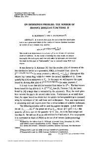
x1 = x 2
x3 x 4 x2
00
01
11
10
0
1
1
0
1
1
1
1
0
0
00
01
11
10
0
0
1
0
1
1
0
1
*
0
x3 x4 x1 x 2
00
01
11
10
00
1
1
0
1
01
0
1
*
0
11
1
1
0
0
10
0
1
0
1
x 1 = x2
x 3 x4 x2
An example of projection of the incompletely specified function f onto the spaces x1 = x2 and x1 = 6 x2 . Fig. 1.
xi 6= p(X (i) ). The projection simply consists in eliminating mi from m. For example, consider the function f shown on the left side of Fig. 1 with fon = {0000, 0001, 0010, 0101, 1001, 1010, 1100, 1101} and fdc = {0111}. Let p be the simple Boolean function x2 , and xi be x1 . The Boolean space {0, 1}4 can be partitioned in the two sets: x1 = x2 and x1 6= x2 each containing 23 points. The projections of f onto these two sets are fon |x1 =x2 = {000, 001, 010, 100, 101} , fdc |x1 =x2 = ∅, and fon |x1 6=x2 = {101, 001, 010}, fdc |x1 6=x2 = {111}. Secondly, observe that these projections do not preserve the Hamming distances among minterms, since we eliminate the variable xi from each minterm, and two minterms projected onto the same subset could have different values for xi . The Hamming distance is preserved only if the function p(X (i) ) is a constant, that is when the (xi , p)-decomposition corresponds to the classical Shannon decomposition. The fact that the Hamming distances may change could be useful when f is represented in SOP form, as bigger cubes could be built in the projection sets. For example, consider again the function f shown on the left side of Fig. 1. The points 0000 and 1100 contained in fon have Hamming distance equal to 2, and thus cannot be merged in a cube, while their projections onto the space fon |x1 =x2 (i.e., 000 and 100, respectively) have Hamming distance equal to 1, and they form the cube x3 x4 . On the other hand, the cubes intersecting both subsets xi = p(X (i) ) and xi 6= p(X (i) ) are divided into two smaller subcubes. For instance, in our running example, the cube x3 x4 of function fon is split in the two sets x1 = x2 and x1 6= x2 forming a cube in fon |x1 =x2 and one in fon |x1 6=x2 , as shown on the right side of Fig. 1. Observe that the cubes eventually split can contain pairs of minterms, whose projections onto the two sets are identical. In our example, x3 x4 is the cube corresponding to the points {0001, 0101, 1001, 1101}, where 0001 and 1101 are projected onto fon |x1 =x2 and become 001 and 101, respectively, and 0101 and 1001 are projected onto fon |x1 6=x2 and again become 101 and 001, respectively. Therefore, we can characterize the set of these minterms as I = f |xi =p ∩ f |xi 6=p . Note that the points in I do not depend on xi . In our example
Ion = fon |x1 =x2 ∩ fon |x1 6=x2 = {001, 010, 101}, and Idc = ∅. In order to overcome some splitting cubes, we could keep I unprojected, and project only the points in f |xi =p \ I and f |xi 6=p \ I, obtaining the expression f = (xi ⊕ p)(f |xi =p \ I) + (xi ⊕ p)(f |xi 6=p \ I) + I. However, we are left with another possible drawback: some points of I could also belong to cubes covering points of f |xi =p and/or f |xi 6=p , and their elimination could cause the fragmentation of these cubes. Thus, eliminating these points from the projected subfunctions would not be always convenient. On the other hand, some points of I are covered only by cubes entirely belonging to I. Therefore keeping them both in I and in the projected subfunctions would be useless and expensive. In our example, since Ion = {001, 010, 101}, in fon |x1 =x2 001 and 101 are useful for forming, together with 000 and 100, the cube x3 ; instead the point 010 is useless and must be covered with an additional cube. The solution of this problem is to project the points belonging to I as don’t cares for f |xi =p and f |xi 6=p , in order to choose only the useful cubes. We therefore propose the following more refined decomposition, using the notation h = (hon , hdc ) for an incompletely specified function h and its on-set hon and don’t care set hdc . Definition 3: Let f (X) be an incompletely specified Boolean function, xi ∈ X, and p(X (i) ) be a completely specified Boolean function. The (xi , p)-decomposition with intersection of f = (fon , fdc ) is the algebraic expression f = (xi ⊕ p)f˜|x =p + (xi ⊕ p)f˜|x 6=p + I , i
i
where f˜|xi =p = (fon |xi =p \ Ion , fdc |xi =p ∪ Ion ) , f˜|xi 6=p = (fon |xi 6=p \ Ion , fdc |xi 6=p ∪ Ion ) , I = (Ion , Idc ) , with Ion = fon |xi =p ∩fon |xi 6=p and Idc = fdc |xi =p ∩fdc |xi 6=p . For our example, the projections of f become f˜|x1 =x2 = (fon |x1 =x2 \ Ion , fdc |x1 =x2 ∪ Ion ) = ({000, 100}, {001, 010, 101}) and f˜|x1 6=x2 = (fon |x1 6=x2 \ Ion , fdc |x1 6=x2 ∪ Ion ) = (∅, {111} ∪ {001, 010, 101}). The Karnaugh maps of this decomposition are show in Fig. 2. Observe that, fixing the function p and a variable x, these decompositions are canonical. We now study these decomposition methods for some choices of the function p. a) Case p = 0.: As we have already observed, if p is a constant function, then the (xi , p)-decomposition is indeed the classical Shannon decomposition: f = xi f |xi =0 + xi f |xi =1 . Recall that (xi ⊕ 0) is equivalent to xi , while (xi ⊕ 0) is equivalent to xi . Also observe that choosing p = 1 we would get exactly the same form. For the (xi , p)-decomposition with intersection we have the following particular form: f = xi f˜|xi =0 + xi f˜|xi =1 + I . Observe that in this particular case, the set I is I
= f (x1 , . . . , xi−1 , 0, xi+1 , . . . , xn ) ∩ f (x1 , . . . , xi−1 , 1, xi+1 , . . . , xn ) .
x3 x 4
x1 = x 2 x2
00
01
11
10
0
1
*
0
*
1
1
*
0
0
I
x3 x 4 x2
x1 = x 2
x3 x4 x2 0
1
00
01
11
10
00
01
11
10
0
0
1
0
1
0
*
0
*
1
0
1
0
0
*
*
0
0
Fig. 2. An example of projection with intersection of the function f of Fig. 1 onto the spaces x1 = x2 and x1 6= x2 .
This implies the following property. Proposition 1: The characteristic function χI of I is the biggest subfunction of f that does not depend on xi . Proof: Let χ1 , . . . , χk be the subfunctions of f that do not depend on xi , and let χ be their union, i.e., χ = χ1 +χ2 + . . . + χk . Observe that χ is still a subfunction of f and it does not depend on xi . Therefore χ is the biggest subfunction that does not depend on xi . We must show that χ = χI . First note that χI is one of the functions χ1 , . . . , χk . Suppose χI = χj , 1 ≤ j ≤ k. By construction, χj is a subfunction of χ. On the other hand, if χ(X) = 1, then there exists an index h such that χh (X) = 1. Since χh does not depend on xi , we have χh (x1 , . . . , xi−1 , 1, xi+1 , . . . , xn ) = = χh (x1 , . . . , xi−1 , 0, xi+1 , . . . , xn ) = 1 . Moreover, since χh is a subfunction of f , on the same input X we have that f (x1 , . . . , xi−1 , 1, xi+1 , . . . , xn ) = = f (x1 , . . . , xi−1 , 0, xi+1 , . . . , xn ) = 1 . This implies that χj (X)
= f (x1 , . . . , xi−1 , 1, xi+1 , . . . , xn ) ∩ f (x1 , . . . , xi−1 , 0, xi+1 , . . . , xn ) = 1 ,
which means that χ is a subfunction of χj . As χj = χI , we finally have that χ = χI . Note that if χI is equal to f , then f does not depend on xi . We conclude the analysis of this special case observing how the (xi , 0)-decomposition, i.e., the classical Shannon decomposition, and the (xi , 0)-decomposition with intersection show a different behavior when the subfunctions f |xi =0 , f |xi =1 , f˜|xi =0 , f˜|xi =1 , and the intersection I are represented as sums of products. Consider a minimal sum of products SOP (f ) for the function f . The number of products in SOP (f ) is always less or equal to the overall number of products in the minimal SOP representations for f |xi =0 and f |xi =1 . This easily follows from the fact that each product in SOP (f ) that does not depend on xi is split into two products, one belonging to a minimal SOP for f |xi =0 and the other belonging to a minimal SOP for f |xi =1 . On the other hand, the (xi , 0)-decomposition
x1 " x i-1 x i+1 " xn x1 " x i-1 x i+1 " xn
x1 " x i-1 x i+1 " xn
SOP for f |x i = p
x1 " x i-1 x i+1 " xn
AND
SOP for p
SOP for f ' |x i = p
AND
SOP for p XOR
f XOR
xi
f
OR
xi
AND
AND
x1 " x i-1 x i+1 " xn
SOP for f |x i ! p
x1 " x i-1 x i+1 " xn x1 " x i-1 x i+1 " xn
OR
SOP for f ' |x i ! p
SOP for I !
Fig. 3.
P-circuit (left) and P-circuit with intersection (right).
with intersection contains the same number of products as SOP (f ), and its overall number of literals is less or equal to the number of literals in SOP (f ). Theorem 1: An (xi , 0)-decomposition with intersection for a function f , where f˜|xi =0 , f˜|xi =1 , and I are represented as minimal sums of products, contains an overall number of products equal to the number of products in a minimal SOP for f , and an overall number of literals less or equal to the number of literals in a minimal SOP forf . Proof: First observe how we can build minimal SOP representations for f˜|xi =0 , f˜|xi =1 , and I starting from a minimal SOP SOP (f ) for f . Indeed, the sum of the projections of all products in SOP (f ) containing the literal xi gives a minimal SOP for f˜|xi =1 , the sum of the projections of all products in SOP (f ) containing the literal xi gives a minimal SOP for f˜|xi =0 , while all remaining products, that do not depend on xi or xi , give a minimal SOP covering exactly the points in the intersection I. The minimality of these SOPs follows from the fact that the (xi , 0)-decomposition with intersection does not change the Hamming distances among the minterms, so that no bigger cubes could be built in the projection sets. Let us now analyze the overall number of literals in the (xi , 0)-decomposition with intersection built from SOP (f ). Let `SOP denote the number of literals in SOP (f ). The products in the SOP for I are left unchanged, so that their overall number of literals `I is preserved. Suppose that r products in SOP (f ) contain xi , and let `xi denote their overall number of literals. The projection of these r products forms a SOP for f˜|xi =1 , whose number of literals is equal to `xi − r, as projecting a product simply consists in eliminating xi from it. Analogously, if s products in SOP (f ) contain xi , and `xi is their overall number of literals, the SOP for f˜|xi =0 contains `xi − s literals. Thus, the (xi , 0)-decomposition with intersection contains exactly `I + `xi − r + `xi − s + 2 = `SOP − r − s + 2 literals, where the two additional literals represent the characteristic functions of the projection sets. b) Case p = xj .: For p = xj , with j 6= i, the two decomposition techniques are based on the projection of f onto the two complementary subspaces of {0, 1}n where xi = xj and xi 6= xj . For the (xi , xj )-decomposition we get the following expression f = (xi ⊕xj )f |xi =xj +(xi ⊕xj )f |xi 6=xj ,
while the (xi , xj )-decomposition with intersection is given by f = (xi ⊕ xj )f˜|xi =xj + (xi ⊕ xj )f˜|xi 6=xj + I, where f˜|xi =xj = (fon |xi =xj \ Ion , fdc |xi =xj ∪ Ion ) , f˜|xi 6=xj = (fon |xi 6=xj \ Ion , fdc |xi 6=xj ∪ Ion ) , with Ion = fon |xi =xj ∩ fon |xi 6=xj and Idc = fdc |xi =xj ∩ fdc |xi 6=xj . These expressions share some similarities with the EXOR Projected Sum of Products studied in [3]. In particular, if we represent the subfunctions as sums of products, the (xi , xj )-decomposition corresponds to an EP-SOP form, while the (xi , xj )-decomposition with intersection is only partially similar to an EP-SOP with remainder form [3]. The differences between the two expressions are due to the presence of don’t cares in f˜|xi =xj and f˜|xi 6=xj , and to the fact that the intersection I does not depend on the variable xi , while the remainder in an EP-SOP may depend on all the n input variables. Also observe that, thanks to the presence of don’t cares, the (xi , xj )-decomposition with intersection has a cost less or equal to that of an EP-SOP with remainder. c) Cases p = xj ⊕ xk and p = xj xk .: In general the function p used to split the Boolean space {0, 1}n may depend on all input variables, but xi . In this paper we consider only two special cases, based on the use of two simple functions: an EXOR and an AND of two literals. The partition of {0, 1}n induced by the EXOR function does not depend on the choice of the variable complementations. Indeed, since xj ⊕ xk = xj ⊕ xk , and (xj ⊕ xk ) = xj ⊕ xk = xj ⊕ xk , the choices p = xj ⊕ xk and p = xj ⊕ xk give the same partition of the Boolean space. On the contrary, the partition of {0, 1}n induced by the AND function changes depending on the choice of the variable complementations, so that four different cases must be considered: 1) p = xj xk , corresponding to the partition into the sets where xi = xj xk and xi 6= xj xk , i.e., xi = xj + xk ; 2) p = xj xk , corresponding to the partition into the sets where xi = xj xk and xi 6= xj xk , i.e., xi = xj + xk ; 3) p = xj xk , corresponding to the partition into the sets where xi = xj xk and xi 6= xj xk , i.e., xi = xj + xk ; 4) p = xj xk , corresponding to the partition into the sets where xi = xj xk and xi 6= xj xk , i.e., xi = xj + xk . When the subfunctions are represented as SOPs, the resulting decomposition forms share some similarities with the Projected Sum of Products (P-SOP) introduced in [2]. Again, the
Synthesis of P -Circuits
Synthesis of P -Circuits with intersection
INPUT: Functions f and p, and a variable xi OUTPUT: An optimal P -circuit for the (xi , p)-decomposition of f NOTATION: let f = (fon , fdc ), i.e., fon is the on-set of f , and fdc is the don’t care-set of f ,
INPUT: Functions f and p, and a variable xi OUTPUT: An optimal P -circuit for the (xi , p)-decomposition with intersection of f NOTATION: let f = (fon , fdc ), i.e., fon is the on-set of f , and fdc is the don’t care-set of f ,
(=) fon = fon |xi =p ; (6=) fon = fon |xi 6=p ; (=) fdc = fdc |xi =p ; (6=) fdc = fdc |xi 6=p ; (=) (=) M inSOP (=) = OptSOP (fon , fdc ); // optimal SOP for f (=) (6=) (6=) M inSOP (6=) = OptSOP (fon , fdc ); // optimal SOP for f (6=) M inSOP p = OptSOP (p, ∅); // optimal SOP for p P -circuit = (xi ⊕ M inSOP p )M inSOP (=) + (xi ⊕ M inSOP p )M inSOP (6=) return P -circuit
Ion = fon |xi =p ∩ fon |xi 6=p ; Idc = fdc |xi =p ∩ fdc |xi 6=p ; (=) fon = fon |xi =p \ Ion ; (6=) fon = fon |xi 6=p \ Ion ; (=) fdc = fdc |xi =p ∪ Ion ; (6=) fdc = fdc |xi 6=p ∪ Ion ; (=) (=) M inSOP (=) = OptSOP (fon , fdc ); // optimal SOP for f (=) (6=) (6=) M inSOP (6=) = OptSOP (fon , fdc ); // optimal SOP for f (6=) M inSOP I = OptSOP (Ion , Idc ); // optimal SOP for I = (Ion , Idc ) M inSOP p = OptSOP (p, ∅); // optimal SOP for p P -circuit = (xi ⊕ M inSOP p )M inSOP (=) + (xi ⊕ M inSOP p )M inSOP (6=) + M inSOP I return P -circuit
Fig. 4.
Algorithm for the optimization of P-circuits.
Fig. 5. Algorithm for the optimization of P-circuits with intersection.
two forms are different thanks to the presence of don’t cares in the subfunctions, and to the fact that the intersection I does not depend on xi . III. P- CIRCUITS We now show how the decomposition methods described in Section II can be applied to the logic synthesis of Boolean functions. The synthesis idea is simply that of constructing a network for f using networks for the projection function p, for the subfunctions f |xi =p , f |xi 6=p , f˜|xi =p , and f˜|xi 6=p , and a network for the intersection I as building blocks. Observe that the overall network for f will require an EXOR gate for computing the characteristic functions of the projection subsets, two AND gates for the projections and a final OR gate (see Fig. 3). The function p, the projected subfunctions, and the intersection can be synthesized in any framework of logic minimization. In our experiments we focused on the standard Sum of Products synthesis, i.e., we represented p, f |xi =p , f |xi 6=p , f˜|xi =p , f˜|xi 6=p , and I as sums of products. In this way we derived networks for f which we called Projected Circuit and Projected Circuit with Intersection, in short PCircuits, see Fig. 3. If the SOPs representing p, f |xi =p , f |xi 6=p , f˜|xi =p , f˜|xi 6=p , and I are minimal, the corresponding circuits are called Optimal P-Circuits. For instance, the function in Figures 1 and 2 has minimal SOP form x1 x2 x3 + x1 x2 x3 + x3 x4 + x2 x3 x4 , while its corresponding optimal P-circuit is (x1 ⊕ x2 )x3 + x3 x4 + x2 x3 x4 . The number of logic levels in a P-circuit varies from four to five: it is equal to four whenever the SOP for p consists in just one product, and it is equal to five otherwise. If we consider now the power consumption, we can observe in Fig. 3 that xi , i.e., the variable with the highest switching frequency, is connected near the output of the overall logic network, thus triggering a sequence of switching events only for the last four gates. In this way, the contribution of xi to the total power consumption is limited. Finally, we observe that it is possible to apply recursively this decomposition when more than one variable switches with high frequency.
Without Intersection VAR XOR AND 32% 22% 28%
Constant 79%
With Intersection VAR XOR 59% 50%
AND 58%
TABLE I
P ERCENTAGE OF P- CIRCUITS , OVER ALL THE BENCHMARKS , HAVING SMALLER AREA THAN THE P- CIRCUITS BASED ON S HANNON DECOMPOSITION .
A. Synthesis Algorithms We now describe two algorithms for computing optimal Pcircuits, without and with intersection. Both algorithms can be implemented using OBDD data structures [7] for Boolean function manipulation, and a classical SOP minimization procedure (e.g., ESPRESSO [5]). Figures 4 and 5 show the algorithms for the optimization of a P-circuit without and with intersection, respectively. The complexity of the algorithms depends from two factors: the complexity of OBDD operations, which is polynomial in the size of the OBDDs for the operands f and p, and the complexity of SOP minimization. Exact SOP minimization is exponential in time, but efficient heuristics are available (i.e., ESPRESSO in the heuristic mode). IV. E XPERIMENTAL R ESULTS In this section we report experimental results for the two decomposition methods described in the previous sections. The methods have been implemented in C, using the CUDD library for OBDDs to represent Boolean functions. The experiments have been run on a Pentium 1.6GHz CPU with 1 GByte of main memory. The benchmarks are taken from LGSynth93 [14]. We report in the following a significant subset of the functions as representative indicators of our experiments. In order to evaluate the performances of these new synthesis methods, we compare the area of different versions of P-circuits with P-circuits based on the classical Shannon decomposition, i.e., P-circuits representing (xi , 0)decomposition without intersection (referred as Shannon in Table II). In particular we report P-circuits for the following choices of the projection function p: 1) p = 0, decomposi-
Bench add6 alu2 amd b12 dk17 ex7 f51m m181 max1024 max46 mp2d p1 root spla sym10 t1 t2 test1 tial vtx1 x9dn Z5xp1 Z9sym
Shannon Area Time 908 0.65 355 0.45 1620 0.17 227 0.11 263 0.10 436 0.12 497 0.09 227 0.42 2534 0.34 297 0.03 355 0.09 724 0.18 416 0.05 2239 0.79 559 0.30 905 0.83 501 0.06 1465 0.34 3430 5.33 430 0.09 530 0.22 479 0.08 464 0.17
Area 507 382 1694 306 250 463 706 308 2511 301 435 781 594 2570 414 951 589 1488 3337 445 528 593 288
Without Intersection VAR XOR Time Area Time 5.19 669 24.58 0.79 416 3.60 1.24 1800 8.65 0.55 401 4.27 0.38 291 1.82 1.04 492 8.30 0.21 640 0.64 0.58 404 4.44 1.97 2973 8.74 0.14 291 0.41 0.61 508 4.47 0.96 821 3.07 0.14 393 0.50 7.88 3142 74.99 0.64 309 2.92 3.52 1186 41.02 0.65 686 6.37 1.06 1565 3.13 23.68 4062 159.84 1.89 501 32.57 2.23 595 30.62 0.12 743 0.33 0.33 267 1.15
AND Area 524 356 1747 340 230 472 528 341 2642 286 455 842 385 2886 416 982 618 1510 3823 585 548 547 371
Time 90.84 12.93 30.31 15.90 6.85 29.07 2.24 16.39 30.72 1.75 16.49 10.77 1.91 273.75 14.31 155.28 22.95 11.43 557.19 107.74 116.64 1.24 6.07
Constant Area Time 672 0.51 283 0.18 1012 0.12 199 0.18 263 0.06 327 0.09 277 0.09 199 0.08 2980 0.25 307 0.02 276 0.16 711 0.20 417 0.02 2428 0.73 568 0.27 463 0.61 358 0.05 1535 0.25 3368 3.29 390 0.14 412 0.19 324 0.03 379 0.17
VAR Area 814 308 1085 248 250 360 290 252 3043 289 357 777 536 2761 529 510 406 1645 3319 499 401 369 391
With Intersection XOR Area Time 759 23.70 310 4.72 1202 10.88 367 5.25 291 1.99 393 10.39 314 0.85 341 6.65 2977 10.13 294 0.46 411 6.82 847 3.74 602 0.55 3249 84.11 551 3.90 655 78.07 469 9.80 1583 3.66 3952 215.08 486 50.57 457 57.18 441 0.41 395 1.68
Time 4.44 1.03 1.55 0.65 0.46 1.56 0.28 0.68 2.12 0.10 0.75 1.18 0.17 8.82 0.96 6.06 0.88 1.18 31.12 3.03 4.26 0.19 0.64
AND Area 651 298 1180 292 230 364 323 288 2829 293 359 818 446 3107 554 585 416 1484 3827 524 418 302 393
Time 80.93 16.79 37.65 18.13 7.21 38.51 4.11 29.20 34.28 2.14 22.56 13.66 1.94 336.30 16.81 277.38 22.33 13.50 741.85 171.45 217.77 1.29 9.28
TABLE II
C OMPARISON OF AREA AND SYNTHESIS TIME OF P- CIRCUITS REPRESENTING (x0 , p)- DECOMPOSITION FORMS FOR DIFFERENT CHOICES OF THE PROJECTION FUNCTION p.
tion with intersection (referred as Constant in Table II); 2) p = xj , decomposition without and with intersection (VAR in Table II); 3) p = xj ⊕ xk , decomposition without and with intersection (XOR in Table II); 4) p = xj xk , decomposition without and with intersection, choosing the complementations of variables giving the best area (AND in Table II). After the projection, all SOP components of the P -circuits have been synthesized with multi-output synthesis using ESPRESSO in the heuristic mode. Finally, to evaluate the obtained circuits, we ran our benchmarks using the SIS system with the MCNC library for technology mapping and the SIS command map -W -f 3 -s. In Table II we compare mapped area and synthesis time (in seconds) of P -circuits representing decomposition forms without and with intersection for a subset of the benchmarks. Due to space limitation, the results shown refer only to decompositions with respect to the first input variable, x0 , of each benchmark. In all the experiments we considered decompositions with respect to each input variable of each benchmark. The results, summarized in Tab. I, are quite promising. These results support the conclusion that decompositions with intersection provide better results, and that the best choice for the projection function p is the simplest: p = 0. Moreover synthesis for p = 0 with intersection is very efficient in computational time. When p is not constant, the synthesis is time-consuming, since the algorithm must choose the best combination of variables to be utilized for p. Altogether, only 14% of the P-circuits achieve the smallest area when implemented based on the classical Shannon decomposition. V. C ONCLUSION In conclusion, we presented a new method to decompose Boolean functions via complex cofactoring. Experimental results show that this decomposition yields more compact circuits than those obtained with Shannon decomposition. This decomposition has the advantage to minimize the dynamic power dissipation with respect to a known input signal
switching with high frequency. In future work, we plan to verify this property with a transistor level simulation of the circuits. Widely used data structures (i.e., OBDDs) are based on Shannon decomposition. Thus a future development of this work could be the definition of new data structures based on the proposed decomposition. R EFERENCES [1] L. Benini and G. D. Micheli, “Logic Synthesis for Low Power,” in Logic Synthesis and Verification, S. Hassoun and T. Sasao, Eds. Kluwer Academic Publishers, 2002, pp. 197–223. [2] A. Bernasconi, V. Ciriani, and R. Cordone, “On Projecting Sums of Products,” in 11th Euromicro Conference on Digital Systems Design: Architectures, Methods and Tools, 2008. [3] ——, “The Optimization of kEP-SOPs: Computational Complexity, Approximability and Experiments,” ACM Trans. on Design Automation of Electronic Systems, vol. 13, no. 2, 2008. [4] J. C. Bioch, “The complexity of modular decomposition of boolean functions,” Discrete Applied Mathematics, vol. 149, no. 1-3, pp. 1–13, 2005. [5] R. Brayton, G. Hachtel, C. McMullen, and A. Sangiovanni-Vincentelli, Logic Minimization Algorithms for VLSI Synthesis. Kluwer Academic Publishers, 1984. [6] F. Brown, Boolean Reasoning. Kluwer Academic Publishers, 1990. [7] R. Bryant, “Graph Based Algorithm for Boolean Function Manipulation,” IEEE Trans. on Computers, vol. 35, no. 9, pp. 667–691, 1986. [8] J. Cortadella, “Timing-Driven Logic Bi-Decomposition,” IEEE Trans. on CAD of Integrated Circuits and Systems, vol. 22, no. 6, pp. 675–685, 2003. [9] P. Kerntopf, “New Generalizations of Shannon Decomposition,” in Int. Workshop on Applications of Reed-Muller Expansion in Circuit Design, 2001, pp. 109–118. [10] L. Lavagno, P. C. McGeer, A. Saldanha, and A. L. SangiovanniVincentelli, “Timed Shannon Circuits: a Power-Efficient Design Style and Synthesis Tool,” in DAC, 1995, pp. 254–260. [11] P. C. McGeer, R. K. Brayton, A. L. Sangiovanni-Vincentelli, and S. Sahni, “Performance Enhancement through the Generalized Bypass Transform,” in ICCAD, 1991, pp. 184–187. [12] M. Pedram, “Power Estimation and Optimization at the logic level,” Int. Journal of High Speed Electronics and Systems, vol. 5, no. 2, pp. 179–202, 1994. [13] C. Soviani, O. Tardieu, and S. A. Edwards, “Optimizing Sequential Cycles through Shannon Decomposition and retiming,” in DATE, 2006, pp. 1085–1090. [14] S. Yang, “Logic synthesis and optimization benchmarks user guide version 3.0,” Microelectronic Center, User Guide, 1991.