Jul 21, 2016 - lations and discussion throughout the paper leading to a small bi-level optimization ..... surfaces li(x) before and after taking a small step on all.
On Differentiating Parameterized Argmin and Argmax Problems with Application to Bi-level Optimization Stephen Gould1,2 , Basura Fernando1,3 , Anoop Cherian1,3 , Peter Anderson1,2 , Rodrigo Santa Cruz1,2 , and Edison Guo1,2 1
2
Australian Centre for Robotic Vision Research School of Computer Science, ANU 3 Research School of Engineering, ANU
arXiv:1607.05447v2 [cs.CV] 21 Jul 2016
@anu.edu.au
July 22, 2016
Abstract Some recent works in machine learning and computer vision involve the solution of a bilevel optimization problem. Here the solution of a parameterized lower-level problem binds variables that appear in the objective of an upper-level problem. The lower-level problem typically appears as an argmin or argmax optimization problem. Many techniques have been proposed to solve bi-level optimization problems, including gradient descent, which is popular with current end-to-end learning approaches. In this technical report we collect some results on differentiating argmin and argmax optimization problems with and without constraints and provide some insightful motivating examples.
1
Introduction
Bi-level optimization has a long history of study dating back to the early 1950s and investigation of the so-called Stackelberg model [Bard, 1998]. In this model, two players—a market leader and a market follower—compete for profit determined by the price that the market is willing to pay as a function of total goods produced and each player’s production cost. Recently, bi-level optimization problems have found application in machine learning and computer vision where they have been applied to parameter and hyper-parameter learning [Do et al., 2007, Domke, 2012, Klatzer and Pock, 2015], image denoising [Samuel and Tappen, 2009, Ochs et al., 2015], and most recently, video activity recognition [Fernando and Gould, 2016, Fernando et al., 2016]. A bi-level optimization problem consists of an upper problem and a lower problem. The former defines an objective over two sets of variables, say x and y. The latter binds y as a function of x, typically by solving a minimization problem. Formally, we can write the problem as minimizex f U (x, y) subject to y ∈ argminy0 f L (x, y 0 )
(1)
where f U and f L are the upper- and lower-level objectives, respectively. As can be seen from the structure of the problem, the lower-level (follower) optimizes its objective subject to the
1
value of the upper-level variable x. The goal of the upper-level (leader) is to choose x (according to its own objective) knowing that the lower-level will follow optimally. In one sense the argmin appearing in the lower-level problem is just a mathematical function and so bi-level optimization can be simply viewed as a special case of constrained optimization. In another sense it is useful to consider the structure of the problem and study bi-level optimization in its own right, especially when the argmin cannot be computed in closed-form. As such, many techniques have been proposed for solving different kinds of bi-level optimization problems [Bard, 1998, Dempe and Franke, 2015]. In this technical report we focus on first-order gradient based techniques, which have become very important in machine learning and computer vision with the wide spread adoption of deep neural network models [LeCun et al., 2015, Schmidhuber, 2015, Krizhevsky et al., 2012]. Our main aim is to collect results on differentiating parameterized argmin and argmax problems. Some of these results have appeared in one form or another in earlier works, e.g., Faugeras [1993, §5.6.2–5.6.3] considers the case of unconstrained and equality constrained argmin problems when analysing uncertainty in recovering 3D geometry. However, with the growth in popularity of deep learning we feel it important to revisit the results (and present examples) in the context of first-order gradient procedures for solving bi-level optimization problems. We begin with a brief overview of methods for solving bi-level optimization problems to motivate our results in Section 2. We then consider unconstrained variants of the lower-level problem, either argmin or argmax (in Section 3), and then extend the results to problems with equality and inequality constraints (in Section 4). We include motivating examples with gradient calculations and discussion throughout the paper leading to a small bi-level optimization example for learning a novel softmax classifier in Section 5. Examples are accompanied by supplementary Python code.1
2
Background
The canonical form of a bi-level optimization problem is shown in Equation 1. There are three general approaches to solving such problems that have been proposed over the years. In the first approach an analytic solution is found for the lower-level problem, that is, an explicit function y ? (x) that when evaluated returns an element of argminy f L (x, y). If such a function can be found then we are in luck because we now simply solve the single-level problem minimizex f U (x, y ? (x))
(2)
Of course this problem, may itself be difficult to solve. Moreover, it is not always the case that an analytic solution for the lower-level problem will exist. The second general approach to solving bi-level optimization problems is to replace the lowerlevel problem with a set of sufficient conditions for optimiality (e.g., the KKT conditions for a convex lower-level problem). If we think of these conditions being encapsulated by the function hL (x, y) = 0 then we can solve the following constrained problem instead of the original, minimizex,y f U (x, y) subject to hL (x, y) = 0
(3)
The main difficulty here is that the sufficient conditions may be hard to express and the resulting problem hard to solve. Indeed, even if the lower-level problem is convex, the resulting constrained problem may not be. 1
Available for download from http://users.cecs.anu.edu.au/sgould/.
2
The third general approach to solving bi-level optimization problems is via gradient descent on the upper-level objective. The key idea is to compute the gradient of the solution to the lowerlevel problem with respect to the variables in the upper-level problem and perform updates of the form � U � ∂f ∂f U ∂y x←x−η + (4) ∂x ∂y ∂x (x,y? ) In this respect the approach appears similar to the first approach. However, now the function y ? (x) does not need to be found explicitly. All that we require is that the lower-level problem be efficiently solveable and that a method exists for finding the gradient at the current solution.2 This last approach is important in the context large-scale and end-to-end machine learning applications where first-order (stochastic) gradient methods are often the preferred method. This then motivates the results included in this technical report, i.e., computing the gradients of parameterized argmin and argmax optimization problems where the parameters are to be optimized for some external objective or are themselves the output of some other parameterized function to be learned.
3
Unconstrained Optimization Problems
We begin by considering the gradient of the scalar function g(x) = argminy∈R f (x, y) and follow an approach similar to the implicit differentiation derivation that appears in earlier works (e.g., [Samuel and Tappen, 2009, Faugeras, 1993]). In all of our results we assume that the minimum (or maximum) over y of the function f (x, y) exists over the domain of x. When the minimum (maximum) is not unique then g(x) can be taken as any one of the minimum (maximum) points. Moreover, we do not need for g(x) to have a closed-form representation. Lemma 3.1.: Let f : R × R → R be a continuous function with first and second derivatives. Let g(x) = argminy f (x, y). Then the derivative of g with respect to x is dg(x) fXY (x, g(x)) =− dx fY Y (x, g(x)) . where fXY =
∂2f ∂x∂y
. and fY Y =
∂2f . ∂y 2
Proof.
∴
∂f (x, y) =0 ∂y y=g(x)
(since g(x) = argmin f (x, y))
d ∂f (x, g(x)) =0 dx ∂y
(differentiating lhs and rhs)
(5)
y
(6)
But, by the chain rule, d dx
�
∂f (x, g(x)) ∂y
� =
∂ 2 f (x, g(x)) ∂ 2 f (x, g(x)) dg(x) + ∂x∂y ∂y 2 dx
2
(7)
Note that we have made no assumption about the uniqueness of y ? nor the convexity of f L or f U . When multiple minima of f L exist care needs to be taken during iterative gradient updates to select consistent solutions or when jumping between modes. However, these considerations are application dependent and do not invalidate any of the results included in this report.
3
Equating to zero and rearranging gives the desired result �−1 2 � 2 ∂ f (x, g(x)) ∂ f (x, g(x)) dg(x) =− 2 dx ∂y ∂x∂y fXY (x, g(x)) =− fY Y (x, g(x))
(8) (9)
We now extend the above result to the case of optimizing over vector-valued arguments. Lemma 3.2.: Let f : R × Rn → R be a continuous function with first and second derivatives. Let g(x) = argminy∈Rn f (x, y). Then the vector derivative of g with respect to x is g 0 (x) = −fY Y (x, g(x))−1 fXY (x, g(x)). . . where fY Y = ∇2yy f (x, y) ∈ Rn×n and fXY =
∂ ∂x ∇y f (x, y)
∈ Rn .
Proof. Similar to Lemma 3.1, we have: . fY (x, g(x)) = ∇Y f (x, y)|y=g(x) = 0 d fY (x, g(x)) = 0 dx ∴ fXY (x, g(x)) + fY Y (x, g(x))g 0 (x) = 0 d g(x) = −fY Y (x, g(x))−1 fXY (x, g(x)) dx
(10) (11) (12) (13)
The above lemma assumes that g(x) is parameterized by a single scalar value x ∈ R. It is trivial to extend the result to multiple parameters x = (x1 , . . . , xm ) by performing the derivative calculation for each parameter separately. That is, � � ∇x g(x1 , . . . , xm ) = −fY Y (x, g(x))−1 fX1 Y (x, g(x)) · · · fXm Y (x, g(x)) (14) Note that the main computational challenge of the inverting the n × n matrix fY Y (or decomposing it to facilitate solving each system of n linear equations) only needs to be done once and can then be reused for the derivative with respect to each parameter. Thus the overhead of computing gradients for multiple parameters is small compared to the cost of computing the gradient for just one parameter. Of course if x (or g(x)) is changed (e.g., during bi-level optimization) then fY Y will be different and its inverse recalculated. So far we have only considered minimization problems. However, studying the proofs above we see that they do not require that g(x) be a local-minimum point; any stationary point will suffice. Thus, the result extends to the case of argmax problems as well. Lemma 3.3.: Let f : R × Rn → R be a continuous function with first and second derivatives. Let g(x) = argmaxy∈Rn f (x, y). Then the vector derivative of g with respect to x is g 0 (x) = −fY Y (x, g(x))−1 fXY (x, g(x)). . . where fY Y = ∇2yy f (x, y) ∈ Rn×n and fXY =
∂ ∂x ∇y f (x, y)
Proof. Follows from proof of Lemma 3.2. 4
∈ Rn .
3.1
Example: Scalar Mean
In this section we consider the simple example of finding the point whose sum-of-squared distance to all points in the set {hi (x)}m as a mathematical i=1 is minimized. Writing out the problem P 2 optimization problem we have g(x) = argminy f (x, y) where f (x, y) = m (h i=1 i (x) − y) . Here P m 1 a well-known analytic solution exists, namely the mean g(x) = m i=1 hi (x). Applying Lemma 3.1 we have: fY (x, y) = −2
m X
(hi (x) − y)
(15)
h0i (x)
(16)
fY Y (x, y) = 2m m 1 X 0 hi (x) ∴ g 0 (x) = m
(17)
fXY (x, y) = −2
i=1 m X i=1
(18)
i=1
which agrees with the analytical solution (assuming the derivatives h0i (x) exist).
3.2
Example: Scalar Function with Three Local Minima
The results above do not require that the function f being optimized have a single global optimal point. Indeed, as discussed above, the results hold for any stationary point (local optima or inflection point). In this example we present a function with up to three stationary points and show that we can calculate the gradient with respect to x at each stationary point.3 Consider the function f (x, y) = xy 4 + 2x2 y 3 − 12y 2
(19)
with the following partial first- and second-order derivatives fY (x, y) = 4xy 3 + 6x2 y 2 − 24y 3
fXY (x, y) = 4y + 12xy
(20)
2
(21)
fY Y (x, y) = 12xy 2 + 12x2 y − 24
(22)
Then for any stationary point g(x) of f (x, y), where stationarity is with respect to y for fixed x, we have g 0 (x) = −
g(x)3 + 3xg(x)2 3xg(x)2 + 3x2 g(x) − 6
(23)
Here the gradient describes how each stationary point g(x) moves locally with an infintisimal change in x. If such a problem, with multiple local minima, were to be used within a bilevel optimization learning problem then care should be taken during each iteration to select corresponding solution points at each iteration of the algorithm. 3
Technically the function that we present only has three stationary points when x < −2 �1 has two stationary points at x = −2 43 3 and a unique stationary point elsewhere.
5
4 3
�1
3
or x > 0. It
f(x, y) contour
320.000
160.000
g(x)
4
880960 720800 0 0 0 .00 0 .00 400.048 0 .00 0 .00.00 00 .00640 000.0560
240.000
80.000
0.000
1.0
-16 0.0
3
2
2
1
80.000
0.000
1.5 x
1
00
-80.000
00
2.0
2.5
0
0
f(1.0, y) 80 60 40 20 0 20 40 60 80 100 5 4 3 2 1 0 1 2 3 y
1
1
2
2 3
3
4
4
5 0.5
g'(x)
3
-80.000
-240.0
y
4 3 2 1 0 1 2 3 4 5 0.5
1.0
1.5
2.0
2.5
5 0.5
1.0
1.5
2.0
2.5
Figure 1: Example of a parameterized scalar function f (x, y) = xy 4 +2x2 y 3 −12y 2 with three stationary points for any fixed x > 0. The top-left panel shows a contour plot of f ; the bottom-left panel shows the function at x = 1; and the remaining panels show the three solutions for g(x) = argminy f (x, y) and corresponding gradients g 0 (x) at each stationary point.
The (three) stationary points occur when analytically as
∂f (x,y) ∂y
= 0, which (in this example) we can compute
( g(x) ∈ argmin f (x, y) =
0,
y
−3x2 ±
√
9x4 + 96x 4x
) (24)
which we use when generating the plots below. Figure 1 shows a surface plot of f (x, y) and a slice through the surface at x = 1. Clearly visible in the plot are the three stationary points. The figure also shows the three values for g(x) and their gradients g 0 (x) for a range of x. Note that one of the solutions (i.e., y = 0) is independent of x.
3.3
Example: Maximum Likelihood of Soft-max Classifier
Now consider the more elaborate example of exploring how the maximum likelihood feature vector of a soft-max classifier changes as a function of the classifier’s parameters. Assume m classes and let classifier be parameterized by Θ = {(ai , bi )}m i=1 . Then we can define the likelihood of feature vector x for the i-th class of a soft-max distribution as `i (x) = P (Y = i | X = x; Θ) � 1 = exp aTi x + bi Z(x; Θ) � � P Tx + b where Z(x; Θ) = m exp a is the partition function.4 j j j=1 4
(25) (26)
Note that we use a different notation here to be consistent with the standard notation in machine learning. In particular, the role of x is differs from its appearance elsewhere in this article.
6
The maximum (log-)likelihood feature vector for class i can be found as g i (Θ) = argmax log `i (x) x∈Rn m X � exp aTj x + bj = argmax aTi x + bi − log x∈Rn
(27)
(28)
j=1
whose objective is concave and so has a unique global maximum. However, the problem, in general, has no closed-form solution. Yet we can still compute the derivative of the maximum likelihood feature vector g i (Θ) with respect to any of the model parameters as follows. ∇x log `i (x) = ai − ∇2xx log `i (x) =
m X
`j (x)aj
(29)
j=1 m m XX
m X
j=1 k=1
j=1
`j (x)`k (x)aj aTk −
∂ ∇x log `i (x) = [[i = j]]ek − `j (x)xk ∂ajk m
aj −
X ∂ ∇x log `i (x) = −`j (x) aj − `k (x)ak ∂bj
`j (x)aj aTj
m X
(30)
! `l (x)al
− `j (x)ek
(31)
l=1
! (32)
k=1
where ek is the k-th canonical vector (k-th element one and the rest zero) and [[·]] is the indicator function (or iverson bracket), which takes value 1 when its argument is true and 0 otherwise. P ? ¯= m Letting x? = g i (Θ), H = ∇2xx log `i (x? ) and a k=1 `k (x )ak , we have ( H −1 (`i (x? ) − 1)ek , i=j ∂g i (33) = ? −1 ? ∂ajk ¯ ) + ek ) , i 6= j `j (x )H (xk (aj − a ( 0, i=j ∂g i = (34) ? −1 ∂bj ¯ ) , i 6= j `j (x )H (aj − a ¯ since ∇x log `i (x? ) = 0. where we have used the fact that ai = a Figure 2 shows example maximum-likelihood surfaces for one of the likelihood functions `i (x) from a soft-max distribution over ten classes and two-dimensional feature vectors. The parameters of the distribution were chosen randomly. Shown are the initial surface and the surface after adjusting all parameters in the negative gradient direction for the first feature i dimension, i.e., θ ← θ − ηeT1 ∂g ∂θ where we have used θ to stand for any of the parameters in {aij , bi | i = 1, . . . , 10; j = 1, 2}. This example will be developed further below by adding equality and inequality constraints and then applying it in the context of bi-level optimization.
3.4
Invariance Under Monotonic Transformations
This section explores the idea that the optimal point of a function is invariant under certain transformations, e.g., exponentiation. Let g(x) = argminy f (x, y). Now let f˜(x, y) = ef (x,y) and g˜(x) = argminy f˜(x, y). Clearly, g˜(x) = g(x) (since the exponential function is smooth and monotonically increasing). 7
Likelihood Surface after Negative x1 Gradient Step
Likelihood Surface 6
80
0.06
0
0.0
6
4 5 0.12
0.14
0
4
00
0.1
2
0.05
40
0.0
0
2
4
4
6
?
0.02
4
5
0 0.05
0
25
60
2
0
2
0.0
0.0
0.0 20
4
0.10
0.0 60
40
0.150
0.0
0 0.1 0 0.0
2 4
0
80
0
0.075
0.12 0
2
2
0
2
4
6
?
(a) x = (0.817, 1.73)
(b) x = (−1.42, 1.59)
Figure 2: Example maximum-likelihood surfaces `i (x) before and after taking a small step on all parameters in the negative gradient direction for x?1 .
Computing the gradients we see that f˜Y (x, y) = ef (x,y) fY (x, y) f˜XY (x, y) = ef (x,y) fXY (x, y) + ef (x,y) fX (x, y)fY (x, y)
(36)
f˜Y Y (x, y) = ef (x,y) fY Y (x, y) + ef (x,y) fY2 (x, y)
(37)
(35)
So applying Lemma 3.1, we have g˜0 (x) = −
f˜XY (x, g(x)) f˜Y Y (x, g(x))
(38)
ef (x,g(x)) fXY (x, g(x)) + ef (x,g(x)) fX (x, g(x))fY (x, g(x)) ef (x,g(x)) fY Y (x, g(x)) + ef (x,g(x)) fY2 (x, g(x)) fXY (x, g(x)) + fX (x, g(x))fY (x, g(x)) =− fY Y (x, g(x)) + fY2 (x, g(x)) =−
(39) (cancelling ef (x,g(x)) ) (40)
=−
fXY (x, g(x)) fY Y (x, g(x))
(since fY (x, g(x)) = 0) (41)
= g 0 (x)
(42)
Similarly, now assume f (x, y) > 0 for all x and y, and let f˜(x, y) = log f (x, y) and g˜(x) = argminy f˜(x, y). Again we have g˜(x) = g(x) (since the logarithmic function is smooth and monotonically increasing on the positive reals). Verifying Lemma 3.1, we have 1 fY (x, y) f (x, y) f (x, y)fXY (x, y) − fY (x, y)fX (x, y) f˜XY (x, y) = f 2 (x, y) f (x, y)fY Y (x, y) − fY2 (x, y) f˜Y Y (x, y) = f 2 (x, y) f˜Y (x, y) =
8
(43) (44) (45)
and once again we can set fY (x, g(x)) to zero and cancel terms to get g˜0 (x) = g 0 (x). These examples motivate the following lemma, which formalizes the fact that composing a function with a monotonically increasing or monotonically decreasing function does not change its stationary points. Lemma 3.4.: Let f : R × R → R be a continuous function with first and second derivatives. Let h : R → R be a smooth monotonically increasing or monotoncially decreasing function and let g(x) = argminy h(f (x, y)). Then the derivative of g with respect to x is dg(x) fXY (x, g(x)) =− dx fY Y (x, g(x)) . where fXY =
∂2f ∂x∂y
. and fY Y =
∂2f . ∂y 2
(x,y)) (x,y) Proof. Follows from Lemma 3.1 observing that ∂h(f∂y = h0 (f (x, y)) ∂f∂y by the chain rule 0 and that h (f (x, y)) is always non-zero for monotonically increasing or decreasing h.
4
Constrained Optimization Problems
In this section we extend the results of the argmin and argmax derivatives to problems with linear equality and arbitrary inequality constraints.
4.1
Equality Constraints
Let us introduce linear equality constraints Ay = b into the vector version of our minimization problem. We now have g(x) = argminy:Ay=b f (x, y) and wish to find g 0 (x). Lemma 4.1.: Let f : R × Rn → R be a continuous function with first and second derivatives. Let A ∈ Rm×n and b ∈ Rm . Let y 0 ∈ Rn be any vector satisfying Ay 0 = b and let the columns of F span the null-space of A. Let z ? (x) ∈ argminz f (x, y 0 + F z) so that g(x) = y 0 + F z ? (x). Then �−1 T g 0 (x) = −F F T fY Y (x, g(x))F F fXY (x, g(x)) . . where fY Y = ∇2yy f (x, y) ∈ Rn×n and fXY =
∂ ∂x ∇y f (x, y)
∈ Rn .
Proof.
T
∇z f (x, y 0 + F z)|z=z? (x) = 0
(46)
F T fY (x, g(x)) = 0
(47)
T
0
F fXY (x, g(x)) + F fY Y (x, g(x))F z (x) = 0 0
(48) T
∴ z (x) = −(F fY Y (x, g(x))F ) 0
T
−1
∴ g (x) = −F (F fY Y (x, g(x))F )
T
F fXY (x, g(x))
−1
T
F fXY (x, g(x))
Alternatively, we can construct the g 0 (x) directly as the following lemma shows. 9
(49) (50)
Lemma 4.2.: Let f : R × Rn → R be a continuous function with first and second derivatives. Let A ∈ Rm×n and b ∈ Rm with rank(A) = m. Let g(x) = argminy:Ay=b f (x, y). Let H = fY Y (x, g(x)). Then � � �−1 g 0 (x) = H −1 AT AH −1 AT AH −1 − H −1 fXY (x, g(x)) . . where fY Y = ∇2yy f (x, y) ∈ Rn×n and fXY =
∂ ∂x ∇y f (x, y)
∈ Rn .
Proof. Consider the Lagrangian L for the constrained optimization problem, minimize n y∈R
f (x, y) (51)
subject to Ay = b We have L(x, y, λ) = f (x, y) + λT (Ay − b)
(52)
˜ (x) = (y ? (x), λ? (x)) is a optimal primal-dual pair. Then Assume g � � � � ∇y L(x, y ? , λ? ) fY (x, y ? ) + AT λ? = =0 ∇λ L(x, y ? , λ? ) Ay ? − b � � d fY (x, y ? ) + AT λ? =0 Ay ? − b dx �� � � � � ˜ Y (x) fXY (x, y ? ) fY Y (x, y ? ) AT g =0 + ˜ Λ (x) A 0 g 0 � � � �� � ˜ Y (x) −fXY (x, y ? ) fY Y (x, y ? ) AT g = ∴ ˜ Λ (x) 0 g A 0
(53) (54) (55) (56)
From the first row of the block matrix equation above, we have ˜ Λ (x) ˜ Y (x) = H −1 −fXY (x, y ? ) − AT g g
�
(57)
where H = fY Y (x, y ? ). Substituting into the second row gives � ˜ Λ (x) = 0 AH −1 fXY (x, y ? ) + AT g ˜ Λ (x) = − AH −1 A ∴ g
(58) � T −1
AH −1 fXY (x, y ? )
(59)
which when substituted back into the first row gives the desired result with g(x) = y ? and ˜ Y (x). g 0 (x) = g Note that for A = 0 (and b = 0) this reduces to the result from Lemma 3.2. Furthermore, g 0 (x) is in the null-space of A, which we require if the linear equality constraint is to remain satisfied.
4.2
Inequality Constraints
Consider a family of optimization problems, indexed by x, with inequality constraints. In standard form we have minimizey∈R f0 (x, y) subject to fi (x, y) ≤ 0 i = 1, . . . , m 10
(60)
where f0 (x, y) is the objective function and fi (x, y) are the inequality constraint functions. Let g(x) ∈ Rn be an optimal solution. We wish to find g 0 (x), which we approximate using ideas from interior-point Pm methods [Boyd and Vandenberghe, 2004]. Introducing the log-barrier function φ(x, y) = i=1 log(−fi (x, y)), we can approximate the above problem as P minimizey tf0 (x, y) − m (61) i=1 log(−fi (x, y)) where t > 0 is a scaling factor that controls the approximation (or duality gap when the problem is convex). We now have an unconstrained problem and can invoke Lemma 3.2. For completeness, recall that the gradient and Hessian of the log-barrier function, φ(z) = P m i=1 log(−fi (z)), are given by ∇φ(z) = −
m X i=1
2
∇ φ(z) =
m X i=1
1 ∇fi (z), fi (z)
(62) m
X 1 1 T ∇f (z)∇f (z) − ∇2 fi (z) i i fi (z)2 fi (z)
(63)
i=1
Thus the gradient of an inequality constrained argmin function can be approximated as � �−1 � � tfXY (x, g(x)) − φXY (x, g(x)) g 0 (x) ≈ − tfY Y (x, g(x)) − φY Y (x, g(x))
(64)
In many cases the constraint functions fi will not depend on x and the above expression can be simplified by setting φXY (x, y) to zero.
4.3
Example: Positivity Constraints
We consider an inequality constrained version of our scalar mean example from above, Pm 2 g(x) = argminy∈R i=1 (hi (x) − y) subject to y ≥ 0
(65)
where we have added a positivity constraint on y. This problem has closed-form solution ( ) m 1 X g(x) = max 0, hi (x) (66) m i=1
Following Section 4.2 we can construct the approximation gt (x) = argmin tf (x, y) − log(y)
(67)
y∈R
where f (x, y) =
Pm
i=1 (hi (x)
− y)2 . Applying Lemma 3.1 gives m
X ∂ 1 (tf (x, y) − φ(y)) = −2t (hi (x) − y) − ∂y y ∂2 (tf (x, y) − φ(y)) = −2t ∂x∂y
i=1 m X
h0i (x)
(69)
i=1
∂2 1 (tf (x, y) − φ(y)) = 2tm + 2 ∂y 2 y P 0 2t m 0 i=1 hi (x) ∴ gt (x) = 1 2tm + g(x) 2 11
(68)
(70) (71)
Function
0.25
actual t = 1.0e4 t = 1.0e3 t = 1.0e2
0.20
Gradient
1.0 0.8 0.6
g(x)
g'(x)
0.15 0.10
0.4
0.05
0.2
0.000.20
0.15
0.10
0.05 0.00 x
0.05
0.10
0.15
0.00.20
0.20
0.15
0.10
0.05 0.00 x
0.05
0.10
0.15
0.20
Figure 3: Example graph of both function value and gradient for g(x) = argminy≥0 (x − y)2 and approximations gt (x) = argminy t(x − y)2 − log(y) for different values of t. As t → ∞ the approximation converges to the actual function and gradient. ∂ Note that here we can solve the quadratic equation induced by ∂y (tf (x, y) − φ(y)) = 0 to 0 obtain a closed-form solution of gt (x) and hence gt (x). We leave this as an exercise.
Observe from Equation 71 that as t → ∞, ( P gt0 (x)
=
1 m
m 0 i=1 hi (x)
0
if g(x) > 0 if g(x) = 0
(72)
We demonstrate this example on a special case with m = 1 and h1 (x) = x. The true and approximate function and their gradients are plotted in Figure 3.
4.4
Example: Maximum Likelihood of Constrained Soft-max Classifier
Let us now continue our soft-max example from Section 3.3 by adding constraints on the solution. We begin by adding the linear equality constraint 1T x = 1 to give n �P � ��o m T g i (Θ) = argmaxx∈Rn aTi x + bi − log j=1 exp aj x + bj (73) subject to 1T x = 1 � � Following Lemma 4.2 and letting H † = H −1 − 1T H1−1 1 H −1 11T H −1 we have the following gradients with respect to each parameter, ( H † (`i (x? ) − 1)ek , i=j ∂g i = (74) ? † ? ∂ajk ¯ ) + ek ) , i 6= j `j (x )H (xk (aj − a ( 0, i=j ∂g i = (75) ? † ∂bj ¯ ) , i 6= j `j (x )H (aj − a ¯ are as defined in Section 3.3. where H and a Figure 4 shows the constrained solutions before and after taking a gradient step for the same maximum-likelihood surface as described in Section 3.3. Notice that the solution lies along the 12
0.150
0.125
80
0.06
0
0.0
4 0.14
0
4
6
0.175
Likelihood Surface after Negative x1 Gradient Step
Likelihood Surface 6
2
0.0
0
2
4
0.0
75
40
0.02
0.0
2
50
0.1 0
2
60
0.0 20
4
0.0
0.0 60
40
0.0
0 0.1 0 0.0
2 4
0
80
0
0
0.12 0
2
4
6
25
5
0.0
4
2
?
0
2
4
6
?
(a) x = (0.151, 0.849)
(b) x = (−1.23, 2, 23)
Figure 4: Example maximum-likelihood surfaces `i (x) before and after taking a small step on all parameters in the negative gradient direction for x?1 with constraint 1T x = 1.
line x1 +x2 = 1. Moreover, the sum of gradients for x1 and x2 are zero, i.e., the gradient is in the null-space of 1T . To show this it is sufficient to prove that H † 1 = 0, which is straightforward. Next we consider adding the inequality constraint kxk2 ≤ 1 to the soft-max maximum-likelihood problem. That is, we constrain the solution to lie within a unit ball centered at the origin. The new function is given by m X � g i (Θ) = argmax aTi x + bi − log exp aTj x + bj (76) x∈Rn j=1
2
subject to kxk ≤ 1
(77)
Following Section 4.2 we can compute approximate gradients as ( (H + ∇2 φ(x? ))−1 (`i (x? ) − 1)ek , i=j ∂g i ≈ ? 2 ? −1 ? ∂ajk ¯ ) + ek ) , i = 6 j `j (x )(H + ∇ φ(x )) (xk (aj − a
(78)
and ∂g i ≈ ∂bj
( 0, i=j ? 2 ? −1 ¯) , i = `j (x )(H + ∇ φ(x )) (aj − a 6 j
(79)
¯ are �as defined in Section 3.3, and the second derivative for the log-barrier where H and a φ(x) = log 1 − kxk2 is given by ∇2 φ(x) =
4
(1 −
xx kxk2 )2
T
−
2 In×n 1 − kxk2
(80)
Similar to previous examples, Figure 5 shows the maximum-likelihood surfaces and corresponding solutions before and after taking a gradient step (on all parameters) in the negative x1 direction.
13
0 0.12
4 0.14
0
4
0.1 40
80
0.06
0
0.0
6
0.08 0
Likelihood Surface after Negative x1 Gradient Step
Likelihood Surface 6
2 0.12 0
2
0.0
0
0
2
00
2
0 .04
2
0.1
0
60
0.0 20
4
0.0 6
0.0 60
40
0.0
0 0.1 0 0.0
2 4
0
80
0
4
4
6
0.0
40
40
0.02
0.0
0
4
?
2
0
2
4
6
?
(a) x = (0.467, 0.884)
(b) x = (0.227, 0.973)
Figure 5: Example maximum-likelihood surfaces `i (x) before and after taking a small step on all parameters in the negative gradient direction for x?1 with constraint kxk2 ≤ 1.
5
Bi-level Optimization Example
We now build on previous examples to demonstrate the application of the above results to the problem of bi-level optimization. We consider the constrained maximum-likelihood problem from Section 4.4 with the goal of optimizing parameter to achieve a desired location for the maximum-likelihood feature vectors. We consider a three class problem over two dimensional space. Here we use the constrained version of the problem since for a three class soft-max classifier over two-dimensional space there will always be a direction in which the likelihood tends to one as the magnitude of the maximum-likelihood feature vector x tends to infinity. Let the target location for the i-th maximum-likelihood feature vector be denoted by ti and given. Optimizing the parameters of the classifier to achieve these locations (with the maximumlikelihood feature vectors constrained to the unit ball centered at the origin) can be formalised as m
minimizeΘ subject to
1X kg i (Θ) − ti k2 2 i=1 g i (Θ) = argmax log `i (x; Θ)
(81)
x:kxk2 ≤1
Solving by gradient descent gives updates θ
(t+1)
←θ
(t)
−η
m X
(g i (θ) − ti )T g 0i (θ)
(82)
i=1
for any θ ∈ Θ = {(aij , bi )}m i=1 . Here η is the step size. Example likelihood surfaces for the three classes in our example are shown in Figure 6 for both initial parameters and final (optimized) parameters where we have set the target locations to be evenly spaced around the unit circle. Notice that this is achieved by the final parameter settings. Also shown in Figure 6(c) is the learning curve (in log-scale). Here we see a rapid decrease in the objective in the first 20 iterations and final convergence (to within 10−9 of the optimal value) in under 100 iterations. 14
0.280
2
0
1
2
2
2
1
0.350
0.400
0.450
0.475
1
0
1
2
1
2
2
2
1
0
1
0 1 2
2
2
80
0
0
1
0.4
1
1
1
0.300
2
0.250
0.200
1
2
0.42 0 0 0 . 3 0 . 3 9 0.30 .330 60 0 0
50 0.4
0.325
0
2
2
0.275
0.175
1
0.225
(a) Initial 2
1
0
1
2
objective (log scale)
2
0.325
2
0.375
1
0.425
0
0.440 0.480
1
1
1
0 0 90 0.33 0.36 0.3 0.420
2
0
0 0.45
2
0
1
0.400
1
1
2
0.320
0
2
0.360
1
0.2 85
70 0.2 55 40 25 10 95 0.2 0.2 0.2 0.2 0.1
2
10 1 10 0 10 -1 10 -2 10 -3 10 -4 10 -5 10 -6 10 -7 10 -8 10 -9 10 -10 0
Learning Curve
20
40
iterations
60
80
100
(c) Learning Curve
(b) Final Figure 6: Example bi-level optimization to position maximum-likelihood points on inequality constrained soft-max model. Shown are the initial and final maximum-likelihood surfaces `i (x) for i = 1, 2, 3 and constraint kxk2 ≤ 1 in (a) and (b), respectively. Also shown is the learning curve in (c) where the objective value is plotted on a log-scale versus iteration number.
6
Discussion
We have presented results for differentiating parameterized argmin and argmax optimization problems with respect to their parameters. This is useful for solving bi-level optimization problems by gradient descent [Bard, 1998]. The results give exact gradients but (i) require that function being optimized (within the argmin or argmax) be smooth and (ii) involve computing a Hessian matrix inverse, which could be expensive for large-scale problems. However, in practice the methods can be applied even on non-smooth functions by approximating the function or perturbing the current solution to a nearby differentiable point. Moreover, for large-scale problems the Hessian matrix can be approximated by a diagonal matrix and still give a descent direction as was recently shown in the context of convolutional neural network (CNN) parameter learning for video recognition via stochastic gradient descent [Fernando and Gould, 2016]. The problem of solving non-smooth large-scale bi-level optimization problems, such as in CNN parameter learning for video recognition, present some interesting directions for future research. First, given that the parameters are likely to be changing slowly for any first-order gradient update it would be worth investigating whether warm-start techniques would be effectivey for speeding up gradient calculations. Second, since large-scale problems often employ stochastic gradient procedures, it may only be necessary to find a descent direction rather than the direction of steepest descent. Such an approach may be more computationally efficient, however it is currently unclear how such a direction could be found (without first computing the true gradient). Last, the results reported herein are based on the optimal solution to the lower-level problem. It would be interesting to explore whether non-exact solutions could still lead to descent directions, which would greatly improve efficiency for large-scale problems, especially during the early iterations where the parameters are likely to be far from their optimal values. Models that can be trained end-to-end using gradient-based techniques have rapidly become the leading choice for applications in computer vision, natural language understanding, and other areas of artificial intelligence. We hope that the collection of results and examples included in 15
this technical report will help to develop more expressive models—specifically, ones that include optimization sub-problems—that can still be trained in an end-to-end fashion. And that these models will lead to even greater advances in AI applications into the future.
References J. F. Bard. Practical Bilevel Optimization: Algorithms and Applications. Kluwer Academic Press, 1998. S. P. Boyd and L. Vandenberghe. Convex Optimization. Cambridge, 2004. S. Dempe and S. Franke. On the solution of convex bilevel optimization problems. Computational Optimization and Applications, pages 1–19, 2015. C. B. Do, C.-S. Foo, and A. Y. Ng. Efficient multiple hyperparameter learning for log-linear models. In Advances in Neural Information Processing Systems (NIPS), 2007. J. Domke. Generic methods for optimization-based modeling. In Proc. of the International Conference on Artificial Intelligence and Statistics (AISTATS), 2012. O. Faugeras. Three-dimensional Computer Vision. MIT Press, 1993. B. Fernando and S. Gould. Learning end-to-end video classification with rank-pooling. In Proc. of the International Conference on Machine Learning (ICML), 2016. B. Fernando, P. Anderson, M. Hutter, and S. Gould. Discriminative hierarchical rank pooling for activity recognition. In Proc. of the IEEE Conference on Computer Vision and Pattern Recognition (CVPR), 2016. T. Klatzer and T. Pock. Continuous hyper-parameter learning for support vector machines. In Computer Vision Winter Workshop (CVWW), 2015. A. Krizhevsky, I. Sutskever, and G. E. Hinton. ImageNet classification with deep convolutional neural networks. In Advances in Neural Information Processing Systems (NIPS), 2012. Y. LeCun, Y. Bengio, and G. Hinton. Deep learning. Nature, 521(7553):436–444, 2015. P. Ochs, R. Ranftl, T. Brox, and T. Pock. Bilevel optimization with nonsmooth lower level problems. In International Conference on Scale Space and Variational Methods in Computer Vision (SSVM), 2015. K. G. G. Samuel and M. F. Tappen. Learning optimized MAP estimates in continuously-valued MRF models. In Proc. of the IEEE Conference on Computer Vision and Pattern Recognition (CVPR), 2009. J. Schmidhuber. Deep learning in neural networks: An overview. Neural Networks, 61:85–117, 2015.
16