On Discrete Time Output Feedback Sliding Mode Like Control for Non

Proceedings of the 42nd IEEE Conference on Decision and Control Maui, Hawaii USA, December 2003

TuP11-6

On Discrete Time Output Feedback Sliding Mode Like Control for Non-minimum Phase Systems Nai One Lai, Christopher Edwards and Sarah K. Spurgeon Control Systems Research Group, Department of Engineering University of Leicester University Road, Leicester LE1 7RH, U.K. [email protected]

Abstract— This paper presents a novel approach to the problem of discrete time output feedback sliding mode control design, where the system to be controlled is non-minimum phase. The method described in this paper applies to uncertain (square) systems with matched uncertainties. A connection between previously established output feedback min-max controllers and discrete time sliding mode controllers will be given, which is crucial to the approach presented. A new explicit method will be described to solve a constrained Riccati inequality which allows the calculation of the ultimate boundedness sets associated with the controller. A numerical example from the literature is used to illustrate the results described in the paper.

I. I NTRODUCTION Motivated by recent results in the area of robust output feedback control for discrete, uncertain systems [11], [12], this paper presents new insight into the problem of discrete time sliding mode control (DSMC) for non-minimum phase systems via output feedback. Classically a (continuous time) sliding mode is generated by means of discontinuities in the control signals about a surface in the state-space. The discontinuity surface (sliding surface) is attained from any initial condition in a finite time interval. Provided the controller is designed appropriately, the motion when constrained to the surface (the sliding mode) is completely insensitive to so-called matched uncertainty [14], [4], i.e. any uncertainties that lie within the range space of the input distribution matrix. The (continuous) control action necessary to maintain an ideal sliding motion is known as the equivalent control [14]. This is not the applied control, which is discontinuous, but is a theoretical quantity representing the continuous, average behaviour of the applied control. Traditionally, sliding mode control has been developed in a framework in which all the system states are available. This is not very realistic for practical problems. This motivates the need for output feedback sliding mode controllers. The class of systems for which an output feedback sliding mode approach is applicable is limited. This is because the reduced-order dynamics of the system, whilst sliding, have the invariant zeros of the system amongst the poles of the closed-loop system, and hence unstable transmission zeros will result in unstable sliding mode dynamics [4]. Therefore, non-minimum phase systems normally pose problems in the

0-7803-7924-1/03/$17.00 ©2003 IEEE

development of output feedback sliding mode controllers. In digital control, the sampling of a continuous time signal replaces the original continuous time signal by a sequence of values at discrete time instances. In discrete time, it is not possible in general to attain ideal sliding as the control signal remains constant between sampling times and is computed at discrete instances. Thus the invariance properties of continuous time sliding mode control are lost. The obvious solution of sampling at high frequency, which will closely approximate continuous time, is not always possible. For this reason the idea of DSMC has been proposed in [1], [2], [5], [7], [10], [13]. In this case, the control law needs to be designed to keep the states as close as possible to the sliding surface and the problem becomes one of minimising sensitivity to the system uncertainty. The results presented in [13] show that an appropriate choice of sliding surface, used with the ‘equivalent control’, can guarantee a bounded motion about the surface in the presence of a bounded uncertainty. It was also argued that it is sufficient to use a linear controller, unlike in continuous time sliding mode control, where ideal sliding is usually achieved with a nonlinear discontinuous controller. From this point of view, the DSMC problem can be looked at as a robust optimal control problem. This is the motivation for this paper where the ideas begin with the work of Sharav-Schapiro et al. [11], [12]. This paper proposes a new switching function for square discrete time systems which is applicable to a class of uncertain non-minimum phase systems. Although the switching function may not necessarily be realizable through outputs alone, the associated optimal control law can be. A novel, explicit method for synthesizing an appropriate Lyapunov function will be given which enables estimates of the ultimate boundedness set to be calculated. The structure of the paper is as follows. In Section II, the work of Corless et al. and Sharav-Schapiro et al. will be introduced and some background ideas on min-max controllers will be explained briefly. Section III will describe the controller design strategy for a class of square systems, which may be non-minimum phase. Section IV analyzes the uncertain closed-loop system. An example taken from the literature will be used to further illustrate this method in

1374

Section V. Conclusions will be presented in Section VI.

then as argued in [12], if the closed loop system matrix

The mathematical notation is quite standard. In a matrix context A > B means A − B is positive definite. For a symmetric matrix, λ() and λ() denote the maximum and minimum eigenvalues respectively.

Consider an uncertain discrete time system

•

with matched uncertainties, ξ(k), which are assumed to belong to a ‘balanced set’ [3]1 , and where x ∈ Rn and u ∈ Rm . Assume without loss of generality that H is full rank.

•

Define a Lyapunov function candidate as (2)

where P > 0 is a symmetric positive definite (s.p.d.) matrix. The difference of the function in (2) is defined as 4V (k) = V (k + 1) − V (k)

(3)

(4)

This is referred to as the Lyapunov min-max control law [3]. To realize this control law generally requires all the states of the system. Now consider the system in (1) with a given output y(k) = Cx(k)

(5)

where y ∈ Rp and m = p < n. The system given in (1) and (5) is therefore square. The state feedback min-max control law in (4) can be realized through the outputs if the following additional constraint HT P G = F C

(10)

(6)

Stability of the system matrix Gc is equivalent to the invariant zeros of the system (G, H, C, 2D) being stable. The discrete output min-max controller in (7) does not need the original system (G, H, C) to be minimum phase.

The next section will show how this result can be used to explore the solution of the discrete time sliding mode control problem where the control is to be output based and the system may be non-minimum phase. Furthermore, the connection between output feedback min-max controllers and discrete sliding mode controllers will be established.

The optimal state feedback control law, including all nonlinear state dependent controllers which minimize 4V (k) with respect to u, for the worst case ξ, is given by usmm (k) = −(H T P H)−1 H T P Gx(k)

GTc P Gc − P < 0

Remarks : (1)

V (k) = xT (k)P x(k)

(9)

then the control law in (7) is the unique stabilizing output feedback min-max controller.

II. P RELIMINARIES

x(k + 1) = Gx(k) + H(u(k) + ξ(k))

is stable and

Gc = (G − H(2D)−1 C)

III. O UTPUT DSMC FOR NON - MINIMUM PHASE SYSTEMS Consider initially the nominal system of (1): x(k + 1) = Gx(k) + Hu(k)

(11)

where no uncertainty is present. Furthermore assume: A1) G is nonsingular A2) D := 21 CG−1 H is nonsingular A3) Gc = (G − H(2D)−1 C) is stable. Assumption A1 is not a very stringent assumption and most discrete systems satisfy this requirement. Though not all systems would satisfy assumption A3, it is, however, an easy test to carry out on a given system. Define a switching function, as s(k) = Sx(k)

(12)

is satisfied, where F ∈ Rm×m and is nonsingular [6]. Provided the system matrix G is invertible, after some simple algebraic manipulation, the control law in (4) can be written as uomm (k) = −(CG−1 H)−1 y(k) (7)

where S ∈ Rm×n . The ‘idealized’ sliding surface can be defined as S = {x(k) : Sx(k) = 0} (13)

As in [11], [12] define

It is desirable for the control law to drive the switching function in (12) to zero in finite time. When this happens, an ideal sliding motion is achieved and

D := 1 Suppose

1 CG−1 H 2

(8)

s(k + 1) = s(k) = 0

the uncertainty ξ(k) ∈ F , then F is a balanced set if ξ(k) ∈ F ⇒ −ξ(k) ∈ F

(14)

It follows that s(k + 1) = SGx(k) + SHu(k) = 0

1375

(15)

The ‘equivalent control’ necessary to maintain sliding, obtained by rearranging (15), is therefore ueq (k) = −(SH)−1 SGx(k)

(16)

In the next section, the uncertain system in (1) will be considered and the closed-loop system performance will be analyzed. IV. C LOSED LOOP ANALYSIS OF THE UNCERTAIN SYSTEM

assuming by design det(SH) 6= 0. The ideal closed-loop dynamics are given by substituting the equivalent control into (11): −1

x(k + 1) = Gx(k) − H(SH) SGx(k) = (In − H(SH)−1 S)Gx(k)

(17)

The matrix Ps , (In − H(SH)−1 S) is a projection operator [4] and has a special characteristic whereby its eigenvalues are 1’s and 0’s. The eigenvalues of Ps G will have m poles at the origin and the remaining n−m poles will be the invariant zeros of the system (G, H, S) - for details see the Appendix. Now, substituting the output min-max control law (7) into the nominal system (11), the closed-loop system is x(k + 1) = (In − H(CG−1 H)−1 CG−1 )Gx(k)

(18)

Comparing equation (18) with (17), the two are identical if the switching function matrix S := CG−1 . The ramifications of the choice of switching function s(k) = CG−1 x(k)

(19)

will be explored in the remainder of the paper.

If equation (11) is multiplied on the left and right by S = CG−1 , it follows that s(k + 1)

•

=

In order to facilitate the analysis, a change of coordinates will be introduced. Without loss of generality it can be assumed that the input distribution matrix · ¸ 0 H= (20) H2 where H2 ∈ Rm×m and det(H2 ) 6= 0. This coordinate system is commonly used in the design of sliding mode controllers and is often referred to as ‘regular form’ [14]. From Assumption A1, det(G) 6= 0, and so equation (6) can be written as

Remarks : •

Consider the system in (1) and assume that whilst ξ(k) is unknown, it is norm bounded by a known constant ρ0 . In this uncertain case, an ideal sliding motion cannot exist. Instead, this section will calculate a boundary layer into which the switching states must enter. In order to do this, the s.p.d. matrix P associated with the min-max controller must be calculated. Assume assumptions A1-A3 hold. A novel, explicit construction will now be described for synthesizing the Lyapunov matrix P associated with the output min-max controller in (7).

y(k) + 2Du(k)

where D is defined in (8). So, with the output min-max control law (7), s(k + 1) = 0, and the sliding surface is attained in one time-step, i.e. the system has deadbeat behaviour. This is because of the existence of pole(s) at the origin due to the characteristics of the projection operator. As argued in the Appendix, the reduced order ideal sliding mode is governed by the invariant zeros of the fictitious system (G, H, CG−1 ) and so does not depend on the invariant zeros of (G, H, C).

The key observation of this section is the following: This method of designing DSMC uses output information and for a certain class of systems can solve the problem of designing sliding mode controllers for systems that are nonminimum phase. Although the switching function in (19) is not necessarily realizable using the outputs, it is not required in the optimal output min-max control law (7), which is a function of the outputs. Furthermore, the output feedback min-max controller in (7) is the equivalent control associated with the switching function gain in (19).

H T P = F CG−1 := F S

(21)

where S is defined as in Section III. Suppose in the coordinate system associated with regular form £ ¤ S = S1 S2 (22) where S2 ∈ Rm×m . From Assumption A2, det(SH) =: det(CG−1 H) 6= 0 then using the fact that SH = S2 H2 with det(H2 ) 6= 0, it follows that det(S2 ) 6= 0. Consequently, the coordinate change x 7→ T x = x ¯ where · ¸ In−m 0 T = (23) S1 S2 is invertible. In this new coordinate system · ¸ ¯ ¯ ¯ = T GT −1 = G11 G12 G ¯ 21 G ¯ 22 G · ¸ 0 ¯ H = TH = S 2 H2 £ ¤ −1 ¯ S = ST = 0 I

(24) (25) (26)

¯ 11 ∈ R(n−m)×(n−m) . The structure of H ¯ and S¯ are where G the special features of this canonical form.

1376

In the new set of coordinates, the original Lyapunov matrix P 7→ (T −1 )T P T −1 =: P¯ and equation (21) becomes ¯ T P¯ T = F S¯ H

(27)

¯ and It can easily be seen from (27) and the structures of H ¯ ¯ S in (26) that P must have a block diagonal structure: · ¸ P1 0 ¯ P = (28) 0 P2 (n−m)×(n−m)

where P1 ∈ R F = (S2 H2 )T P2 .

, P2 ∈ R

In this coordinate system ¯ c = (I − H( ¯ S¯H) ¯ −1 S) ¯G ¯= G

·

m×m

¯ 11 G 0

and furthermore

¯ 12 G 0

A family of solutions (P1 , P2 ) to this problem exist. Specifically, let P1 be a solution to

and P1 and P2 satisfy (31) and (33) respectively. Since by straightforward algebraic manipulation (35)

the matrix P satisfies (6) and the discrete Riccati inequality (36)

It can be shown that in the x ¯ coordinates ¯ x(k) + ξ T (S2 H2 )T P2 (S2 H2 )ξ 4V = −¯ x(k)T Q¯

(37)

¯ > 0, 4V < 0 for x Note that if ξ ≡ 0, then since Q ¯ 6= 0. In the uncertain case, asymptotic stability will be lost. To

−V q + rkξk2 −qV + rρ0

(38)

¯ q = λ(P¯ −1 Q) r = λ((S2 H2 )T P2 (S2 H2 )) ½

ΩV =

r x ¯ : V (¯ x) < ρ0 q

¾ (39)

it follows that V (¯ x) > rq ρ0 and hence from (38), 4V is decreasing. Thus ΩV is an invariant set. Note also that in the coordinate system x ¯ the last m states are the switching function states, and so s 1 r ksk < ρ0 λmin (P2 ) q V. E XAMPLE The theory described in the previous sections will now be applied to the system given by Sharav-Schapiro et al. in [11]. Consider the system x(k + 1) = y(k) =

(33)

Thus provided A1-A3 are satisfied, the control law uomm (k) in (7) is a stabilizing min-max controller for the Lyapunov function (2) where ¸ · P1 + S1T P2 S1 S1T P2 S2 T ¯ (34) P := T P T = S2T P2 S1 S2T P2 S2

= ≤

where

(32)

¯ 11 is stable. Such a solution is guaranteed to exist since G Then from the Schur complement, inequality (31) is satisfied if and only if

GT P G − P − GT P H(H T P H)−1 H T P G < 0

4V

Outside the region

which in terms of the partition in (26) can be written as ¸ · ¯ 12 ¯ 11 ¯ T11 P1 G ¯ T11 P1 G −G P1 − G (31) ¯ 12 > 0 ¯ 11 ¯ T P1 G ¯ T P1 G P2 − G −G 12 12

¯ Tc P¯ G ¯c ≡ G ¯ T P¯ G ¯−G ¯ T P¯ H( ¯ H ¯ T P¯ H) ¯ −1 H ¯ T P¯ G ¯ G

which can be written as

(29)

and so by assumption A3 in the previous section, the sub¯ 11 ∈ R(n−m)×(n−m) is stable. The restriction on P¯ matrix G is now that ¯ := P¯ − G ¯ Tc P¯ G ¯c > 0 Q (30)

¯ 12 ) ¯ 11 )−1 (G ¯ T11 P1 G ¯ 11 (P1 − G ¯ T11 P1 G ¯ T12 P1 G P2 > G T ¯ 12 ¯ 12 P1 G +G

¯ + λ((S2 H2 )T P2 (S2 H2 ))kξk2 4V ≤ −V λ(P¯ −1 Q)

and

¸

¯ T11 P1 G ¯ 11 > 0 P1 − G

calculate the ultimate boundedness set (which contains the zero state), consider the worse case bound on the inequality (37):

Gx(k) + H(u(k) + ξ(k)) Cx(k)

which has the following system matrices · ¸ · ¸ £ 0 1 0 G= , H= , C = c0 0.24 0.2 1

c1

(40) (41) ¤

If |c0 /c1 | > 1, the system will be non-minimum phase. In this example, c0 = 2 and c1 = 1 will be considered. In this case, the system triple (G, H, C) satisfies assumptions A1A3 and has an unstable invariant zero at −2. However the invariant zero of the fictitious system (G, H, CG−1 ) is 0.08. Using the ‘classical method’ as in [8], if the sliding surface is picked so that S = C and assuming an ideal sliding motion is induced, i.e s(k) = 0, the associated reduced order sliding motion is governed by −2 and is therefore unstable. This shows that, in this case, the ‘classical choice’ of sliding surface does not solve the control problem for non-minimum phase systems. However, using the choice of sliding surface S = CG−1 in (19), the reduced-order ideal sliding motion is governed by a pole at 0.08. This switching function is not realizable

1377

since CG−1 x(t) requires all state information, however, the optimal control law is and is given by

3

u(k) = −(2D)−1 y(k)

2

1

With the coordinate change · ¸ 1 0 T = −0.6667 8.333

x2(k)

it can be shown that for this example the constraints (32) and (33) become P1 > 0 (42)

0

−1

−2

and P2 > 0.145P1 respectively. Here, the matrix P¯ was chosen to be · ¸ 1 0 ¯ P = 0 0.15

(43) −3 −1.5

−1

−0.5

0

0.5

1

1.5

2

x1(k)

(44)

Fig. 1. Phase plane plot showing the state trajectory (initial conditions [2, 1]) with respect to ultimate boundedness set.

The expression S2 H2 = 8.3333 and simple calculations show · ¸ 0.9936 −0.0096 ¯= Q (45) −0.0096 0.1356

7

6

For this particular example, the components in the expressions which form the radius of the ultimate boundedness set are given by λ((S2 H2 )T P2 S2 H2 ) = 10.4167 and ¯ = 0.8976 . λ(P¯ −1 Q)

5

4

Suppose the system (40)-(41) is subjected to an external disturbance in the form of a sine wave

s(k)

3

2

ξ(k) = 0.1 sin(k)

(46) 1

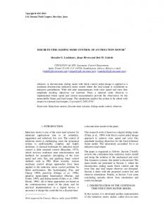
and so the bound on the disturbance ρ0 = 0.1. In this case, the ultimate boundedness set © ª ΩV = x ¯:x ¯T P¯ x ¯ < 1.1605 (47) This is shown in Figure 1 together with the path of the state trajectory for this example. The calculated worst case offset from the sliding function is |s| ≤ 2.7811

0

−1

0

5

10

15

20

25

30

35

40

45

50

t(s)

Plot of switching function against time, with initial conditions [2, 1]. Fig. 2.

(48)

Figure 2 shows a plot of the switching function of the system with the disturbance. The ‘long term’ worst case distance from the sliding function, computed from the simulation is 0.8333. VI. C ONCLUSION In designing discrete time sliding mode controllers which are output based, the existence of unstable transmission zeros in the plant poses a problem. In this paper a link has been made between the design of discrete time sliding mode controllers and a class of output feedback discrete time min-max controllers. A novel switching function is described. This in itself is not realizable through outputs

alone, but it gives rise to a control law which depends only on outputs. The discrete time reduced-order sliding motion associated with this novel choice of switching function is not governed by the invariant zeros of the system - which therefore are not required to be minimum phase. The class of systems to which this approach is applicable is easily identified. A novel method to explicitly solve the constrained Riccati inequality which underpins this approach is given. The resulting s.p.d. matrix can be used to calculate the ultimate boundedness set for the closed-loop system. The design methodology minimizes the deviation from the sliding surface for a maximum bound on the (matched) uncertainty.

1378

ACKNOWLEDGEMENT

This means that

Many thanks to EPSRC for their support and funding, via a Project Studentship (Grant Reference GR/R32901/01). A PPENDIX

det(P (z)) = 0 ⇔ det(zI − (G11 − G12 K)) = 0 Therefore, the invariant zeros of (G, H, S) are the eigenvalues of (G11 − G12 K), i.e poles of the reduced-order sliding motion.

In regular form [14], the nominal system from (11) can be written as x1 (k + 1) = x2 (k + 1) =

G11 x1 (k) + G12 x2 (k) G21 x1 (k) + G22 x2 (k) + H2 u(k)

(49) (50)

where x1 ∈ Rn−m , x2 ∈ Rm , H2 ∈ Rm×m is nonsingular and the matrices G11 , G12 , G21 and G22 are appropriate partitions of the system matrix. The switching function matrix from (12) can be written as £ ¤ S = S1 S2 where S2 ∈ Rm×m is nonsingular. During ideal sliding, Sx(k) = 0, which implies that S1 x1 + S2 x2 = 0. Substituting for x2 in (49) it follows that the ideal sliding motion is given by x1 (k + 1) = (G11 − G12 K)x1 (k) where K = S2−1 S1 . By definition, the transmission zeros of the system (G, H, S) are given by {z ∈ C : P (z) loses normal rank} where Rosenbrock’s system matrix denoted by P (z) [9] is given by · ¸ zI − G H P (z) = −S 0 Rosenbrock’s system matrix loses rank if and only if   zI − G11 −G12 0 −G22 H2  = 0 det(P (z)) = det  −G21 −S1 −S2 0 With the assumption that H2 is nonsingular · ¸ zI − G11 −G12 det(P (z)) = 0 ⇔ det =0 −S1 −S2 and this is equivalent to µ · ¸ ¶ zI − (G11 − G12 K) 0 det L R =0 0 −S2 where L,

·

I 0

G12 S2−1 I

¸

· and

R,

I K

0 I

(51) ¸

VII. REFERENCES [1] C.Y. Chan. Robust discrete-time sliding mode controller. Systems and Control Letters, 23:371–374, 1994. [2] C.Y. Chan. Discrete adaptive sliding mode control of a state-space system with a bounded disturbance. Automatica, 34:1631–1635, 1998. [3] M. Corless. Stabilization of uncertain discrete-time systems. Proc IFAC Workshop on Model Error Concepts and Compensation, Boston, 1985. [4] C. Edwards and S.K. Spurgeon. Sliding Mode Control: Theory and Applications. Taylor & Francis, 1998. [5] K. Furuta. Sliding-mode control of a discrete system. Systems and Control Letters, 14:145–152, 1990. [6] M. E. Magana and S. H. Zak. Robust output feedback stabilization of discrete uncertain dynamical systems. IEEE Transactions on Automatic Control, 33:1082– 1085, 1988. [7] C. Milosavljevic. General conditions for the existence of a quasisliding mode on the switching hyperplane in discrete variable structure systems. Automation and Remote Control, 46:307–314, 1985. [8] G. Monsees. Discrete-Time Sliding Mode Control. PhD thesis, Delft University of Technology, 2002. [9] H. H. Rosenbrock. Computer-Aided Control System Design. Academic Press, 1974. [10] S.Z. Sapturk, Y. Istefanopulous, and O. Kaynak. On the stability of discrete-time sliding mode control systems. IEEE Transactions on Automatic Control, 32:930–932, 1987. [11] N. Sharav-Schapiro, Z. J. Palmor, and A. Steinberg. Robust output feedback stabilizing control for discrete uncertain siso systems. IEEE Transactions on Automatic Control, 41:1377–1381, 1996. [12] N. Sharav-Schapiro, Z. J. Palmor, and A. Steinberg. Output stabilizing robust control for discrete uncertain systems. Automatica, 34:731–739, 1998. [13] S.K. Spurgeon. Hyperplane design techniques for discrete-time variable structure control systems. International Journal of Control, 55:445–456, 1992. [14] V.I. Utkin. Sliding Modes in Control Optimization. Springer-Verlag, Berlin, 1992.

Since the matrices L and R are both independent of z and have determinant equal to unity, (51) is equivalent to · ¸ zI − (G11 − G12 K) 0 det =0 0 −S2

1379