1
On Dynamic Service Function Chain Deployment and Readjustment Junjie Liu, Wei Lu, Fen Zhou, Ping Lu, Zuqing Zhu, Senior Member, IEEE
Abstract—Network Function Virtualization (NFV) is a promising technology to decouple the network functions from dedicated hardware elements, leading to the significant cost reduction in network service provisioning. As more and more users are trying to access their services wherever and whenever, we expect the NFV-related service function chains (SFCs) to be dynamic and adaptive, i.e., they can be readjusted to adapt to the service requests’ dynamics for better user experience. In this paper, we study how to optimize SFC deployment and readjustment in the dynamic situation. Specifically, we try to jointly optimize the deployment of new users’ SFCs and the readjustment of in-service users’ SFCs while considering the trade-off between resource consumption and operational overhead. We first formulate an integer linear programming (ILP) model to solve the problem exactly. Then, to reduce the time complexity, we design a column generation (CG) model for the optimization. Simulation results show that the proposed CG-based algorithm can approximate the performance of the ILP and outperform an existing benchmark in terms of the profit from service provisioning. Index Terms—Network function virtualization (NFV), Service function chain (SFC), Dynamic support, Column generation.
I. I NTRODUCTION
T
RADITIONALLY, service providers rely on middleboxes to realize the network functions that are needed as a part of a specific service [1]. However, this scheme is restricted by the drawbacks of dedicated hardware, which results in difficulties in deployment and maintenance, prolonged time to market, and high expenses, and thus it cannot adapt to the requirements of emerging applications related to cloud computing [2, 3] and big data [4]. To address these issues, network function virtualization (NFV) [5] was proposed to migrate network functions from expensive dedicated hardware to softwaredefined elements by leveraging IT resource virtualization, i.e., processing traffic with virtual network functions (vNFs) [6]. Hence, service providers do not need to worry too much about the hardware environment during service provisioning. Note that, with NFV, we can represent a network service with a series of connected vNFs, i.e., formulating a service function chain (SFC) [7]. This could be challenging for network control and management (NC&M) when the constraints on IT and bandwidth resources need both to be addressed well [8]. Previously, researchers have considered the problem of vNF placement in [9, 10], while the studies in [7, 11, 12] have addressed how to deploy SFCs. Nevertheless, in order to J. Liu, W. Lu, P. Lu, and Z. Zhu are with the School of Information Science and Technology, University of Science and Technology of China, Hefei, Anhui 230027, P. R. China (email:
[email protected]). F. Zhou is with the LIA lab of the University of Avignon, France (email:
[email protected]). Manuscript received on December 1, 2016.
fully explore the advantages of NFV, we have more challenges to work on. For instance, with the rapidly growth of mobile devices, more and more users are trying to access their services wherever and whenever [13]. Consequently, SFCs need to be readjusted to ensure service continuity when the users are moving, and vNFs might be added in or removed from SFCs to adapt to their demands. However, how to set up and readjust SFCs adaptively such that the dynamic nature of user demands can be properly addressed has not been fully explored yet. For SFCs, the optimal deployment of vNFs will change when their users move [14]. Hence, a static SFC deployment scheme can make the paths among the users and their vNFs sub-optimal, which would not only cause unnecessary bandwidth consumption but also degrade user experience. Moreover, the static deployment approaches can not address the situation in which users can change their SFC patterns on-thefly, since the consideration on vNFs reassignment is missing. On the other hand, if we readjust SFC deployment schemes too frequently, the overhead from vNF migrations could become a serious issue [15]. Therefore, for the dynamic SFC deployment and readjustment, we have to carefully balance the tradeoff between resource consumption and operational overhead. This paper studies how to optimize vNFs deployment and reassignment to efficiently orchestrate SFCs in respond to dynamic user demands. Here, as we consider the service provisioning step after the formulation of SFCs, the order of vNFs in each SFC is predetermined. We also assume that an SFC is provisioned for one user and thus each SFC would take the one-dimensional chain topology. Since our network model allows multiple SFCs to share certain vNFs, more complex and two-dimensional vNF graphs are also addressed in our work. However, the SFCs can actually be more generic with more complex and flexible topologies [16, 17], which will be addressed in our future work. For the vNF deployment, we consider the cost of two parts, i.e., IT and bandwidth resource consumption. For the vNF reassignment, we consider the associated operational overhead. To solve the SFC provisioning problem with these considerations, we first formulate an integer linear programming (ILP) model to maximize the service provider’s profit under the resource and operational overhead constraints. Then, to reduce the time complexity, we design a column generation (CG) [18, 19] model for the optimization to approximate the performance of the ILP. In summary, our main contributions are as follows. • We consider a practical network scenario for dynamic SFC deployment and readjustment and formulate an ILP model to solve the optimization exactly. • We design a CG model based on the feasible service
2
provisioning schemes of the users and leverage it to reduce the time complexity of the optimization. The rest of the paper is organized as follows. Section II provides a brief survey on the related work. In Section III, we describe the network model and formulate the problem of dynamic SFC deployment and readjustment. An ILP model is formulated in Section IV to solve the problem exactly, with formal complexity analysis. Section V discusses the CG model for the problem. The performance evaluation is presented in Section VI. Finally, Section VII summarizes the paper. II. R ELATED W ORK Since its inception, NFV has attracted intensive interests from both academia and industry. For comprehensive surveys on it, one is suggested to refer to [20, 21]. Meanwhile, the standardization activities related to NFV are making important progress recently [5], and drafts on the use cases of NFV and the description of SFCs can be found in [22] and [23], respectively. The work in [24, 25] investigated NFV from the perspective of system implementation. Specifically, Martins et al. considered how to realize NFV with ClickOS in [24], while the authors of [25] proposed an informationexchange-management-as-a-service facility as an extension to the standard NFV management framework, which can support information flow establishment, operation, and optimization. The studies in [7, 9, 11, 26–30] have investigated the problems of vNF or SFC deployment from the perspective of resource allocation. Cohen et al. [26] formulated a problem on vNF placement to minimize both the deployment and connection costs of vNFs, and proposed approximation algorithms that could solve it with performance guarantee. However, their studies did not consider the resource constraints of substrate nodes and links. The authors of [9] considered a hybrid scenario in which network services can be provisioned with both the hardware-specified elements and vNFs. A binary search algorithm was designed in [27] to minimize the number of deployed vNFs under the constraint of data-transfer latency. The work in [28] introduced a dynamic programming based heuristic called Viterbi to solve the problem of SFC deployment. The authors of [7] used a context-free language to formulate the problem of SFC deployment as a mixed integer quadratically constrained program model and use the Pareto set analysis to balance the tradeoffs among several optimization goals. Xia et al. [11] studied the problem of vNF placement in optical inter-datacenter (inter-DC) networks and proposed a binary integer programming model to minimize the cost due to optical-electronic-optical conversions. The study in [30] developed a prediction scheme that can forecast NFV’s future resource requirements, with which the service provider can spin up new resources more wisely and/or plan global availability more effectively. Nevertheless, none of the aforementioned studies considered to support dynamic user demands in vNF/SFC deployment. Note that, for the dynamic schemes, the problem of SFC deployment becomes much more complex since the readjustment of vNF/SFC deployment has to be taken into account and we need to balance the tradeoff between resource consumption and operational overhead.
The work in [31–34] have previously addressed dynamic vNF/SFC deployment. In [31], the authors proposed a novel network architecture for cloudlet (i.e., a mobility-enhanced small-scale cloud DC located at the edge of the Internet). Specifically, they assumed that each user communicated with a specific virtual machine (VM) called Avatar in the cloudlet, investigated how to realize live Avatar migration, and proposed a strategy to optimize the tradeoff between data-transfer latency and VM migration overhead. Note that, even though they considered the mobility feature of the users, their problem is fundamentally different from ours. Basically, each SFC consists of multiple connected VM/vNFs and the relation among them has to be considered in the deployment and readjustment of SFCs. The authors of [32] studied the problem of elastic vNF placement problem and tried to balance the trade-off between elastic overhead and resource consumption. However, they assumed that there was only one type of vNFs and did not consider SFC. Note that, deploying an SFC usually involves the orchestration of several vNFs in different types, which apparently makes the problem-solving more complex. Ayoubi et al. [33] designed an availabilityaware resource allocation and reconfiguration framework for the elastic services in failure-prone DC networks. Although they also considered to reconfigure the embedding schemes of virtual network services when the users’ requests change over time, their focus was on providing the highest availability improvement with the lowest reconfiguration cost. Hence, both their network model and optimization objective are different from ours. In [34], the migration scheme of vNF instances (vNFIs) in dynamic SFCs have been studied to minimize the costs from energy consumption and reconfiguration. The authors proposed algorithms to handle the VNFI placement, SFC routing, and VNFI migration in response to the change of user workload. Nevertheless, they did not consider the bandwidth consumption of SFCs when designing their algorithms, which makes their network model also different from ours. Finally, we hope to point out that even though the problem of dynamic SFC deployment looks similar to the virtual network embedding (VNE) problem that has already been studied intensively before [35–39], they are fundamentally different. Basically, in VNE, the virtual networks’ topologies would not change during the embedding, while in dynamic SFC deployment, the actual topology of an SFC can change with the vNF placement. III. P ROBLEM D ESCRIPTION This section describes the network model and formulates the problem of dynamic SFC deployment and readjustment. A. Network Model The network can be denoted as G = (V, E), where V represents the set of nodes S and E is the set of physical links. Here, we assume V = Vd Vs , which means that there are two types of nodes in the network, i.e., the DCs and the switches, and their sets are Vd and Vs , respectively. The switches can be used as the access points for mobile users and they also forward data traffic in the network, while the DCs contain the
3
User 1
IT resources for vNF deployment. Each DC is locally attached to a switch1 . For every link e ∈ E between two adjacent switches, we use Be to denote its bandwidth capacity. The IT resource capacity of a DC v ∈ Vd is denoted as Cv . We use P to represent the set of vNF types that can be instantiated in the DCs, e.g., network address translation (NAT) and firewall. For a p-th type vNF, we denote its IT resource requirement as cp and assume that it can serve np users at most.
We consider a periodical service provisioning scenario in which the service provider can serve new requests or change the provisioning schemes of in-service requests at time instants with a fixed interval in between. Hence, at each service time, the service provider needs to handle two kinds of users. We use Γ1 to represent the set of new users that are at the first time to access the network, while the in-service users are denoted with set Γ2 . We have Γ = Γ1 ∪ Γ2 as the whole set of users to handle. In the service provisioning, the operational overhead of the service provider is mainly from allocating new users to their required vNFs and migrating the services of in-service users to vNFs at new locations. Hence, for each user in Γ, we count how many vNFs the service provider operates for it, and use the total number as its operational overhead. More specifically, for a new user in Γ1 , the operational overhead equals the number of required vNFs in its SFC, while for an in-service user in Γ2 , the operational overhead is the number of migrated and newly added vNFs since the last service time. The objective of dynamic SFC deployment and readjustment is to maximize the service provider’s profit, which is equal to the total profit from the served requests minus the total deployment cost. The major constraints are those on IT and bandwidth resources and operational overhead. It should be noted that certain requests may be blocked due to the lack of resources. To maximize the profit, the service provider needs to utilize both the IT and bandwidth resources properly, i.e., deploying vNFs adaptively in the DCs, and setting up routing paths intelligently to connect the vNFs for formulating the required SFCs for users. 1 In this work, we assume that the bandwidth capacity of the link between a DC and its local switch would never be used up.
Src Data center Switch
1
6
2 5 3
B. User Model
C. Dynamic SFC Deployment and Readjustment
vNF 2
Src
4
User 1
vNF 1
The user i’s service request can be represented by a 5-tuple → hvi , − gi , si , βi , ri i, where vi ∈ Vs is the switch for its current → access, − gi is a vector to denote the required SFC that consists of a sequence of specific vNFs, si ∈ Vd is the source of the traffic flow, βi is the bandwidth requirement on a connection between two adjacent vNFs in the SFC, and ri represents the profit that the service provider gains after serving this request. Hence, to serve the request, the service provider needs to → secure all the required vNFs in − gi by either deploying new ones or reusing the existing ones that are not fully loaded, find a proper routing path that goes through the required vNFs in correct order, and reserve enough bandwidth on the path to satisfy the bandwidth requirement.
vNF 1
vNF 2
(a) SFC provisioning scheme at previous service time.
User 2
vNF 1
Src
vNF 3
vNF 2 vNF 3 Src 1
Src 6
2
5 3
4 vNF 1 User 1
User 2
(b) SFC provisioning scheme at current service time. Fig. 1.
Example on dynamic SFC deployment and readjustment.
Fig. 1 shows an intuitive example on the dynamic SFC deployment. Here, for simplicity, we omit the wireless access points in the figure and assume that each switch can be used as an access point (i.e., wired or wireless) for the users. Fig. 1(a) shows the SFC deployment scheme at the previous service time, where the in-service User 1 accesses the network from Switch 4 and takes an SFC as vNF 1→vNF 2. Hence, to set up the SFC for User 1, the service provider deploys a vNF 1 and a vNF 2 on DCs 3 and 1, respectively. Then, at the current service time, the service provider finds that a new User 2 joins at Switch 5 to request an SFC as vNF 1→vNF 3 and the in-service User 1 changes its access point to Switch 5 but its SFC stays unchanged. Hence, as shown in Fig. 1(b), the service provider decides to migrate the vNF 1 to DC 5 where it can be efficiently shared by Users 1 and 2, and deploys a vNF 3 on DC 6 for User 2. IV. ILP F ORMULATION In this section, we formulate a path-based ILP model to solve the problem of dynamic SFC deployment and readjustment exactly. Parameters: S Vs and Vd • G(V, E): Network topology, where V = Vd and Vs are for the sets of DCs and switches, respectively. • Cv : IT resource capacity of a DC v ∈ Vd . • Be : Bandwidth resource capacity of a link e ∈ E. • Π: Set of pre-calculated paths in G(V, E). – Πu,v : Set of K shortest paths between u and v in G(V, E), where u, v ∈ V and Πu,v ⊂ Π. – π: A path in Π, s(π) and d(π) represent the source and destination of π, respectively, and len(π) denotes the hop-count of π.
4
•
•
•
•
•
– δe,π : A boolean constant to indicate whether a path π uses a link e. If yes, we have δe,π = 1, and 0 otherwise. Hmax : Maximum operational overhead that the service provider can take at each service time. P: Set of supported vNF types in the network. – np : Maximum number of users that a p-th type vNF can serve (p ∈ P). – cp : IT resource consumption of a p-th type vNF. Γ: Set of users to handle at the current service time, which includes both the new ones in Γ1 and the in-service ones in Γ2 . We use |Γ| to denote the total number of users. → hvi , − gi , si , βi , ri i: A 5-tuple to represent the service request of a user i at current service time. – vi : Access switch of a user i, vi ∈ Vs . → – − gi : Required SFC of a user i, which is a vector that consists of a sequence of specific vNFs. ∗ Li : Number of vNFs in the SFC of a user i. For convenience, we treat the access switch of a user as a dummy vNF that consumes 0 IT resource, i.e., the first vNF in each user’s SFC is its access switch while the other ones are real vNFs. Hence, → we have Li = |− gi | + 1. ∗ gi,j,p : A boolean constant that equals 1 if the jth vNF on the SFC of a user i is a p-th type vNF, and 0 otherwise. Since the first vNF is the user’s access switch, we have gi,1,p = 0, ∀i, p. We also assume that there are no duplicated vNFs in a user’s SFC, and thus if j1 6= j2 , we have gi,j1 ,p + gi,j2 ,p 6 1, ∀i, p. – si : The source of the required traffic flow2 , si ∈ Vd . – βi : Bandwidth requirement on a connection between two adjacent vNFs in the SFC of a user i. – ri : Profit that the service provider gains after provisioning the SFC of a user i. hdi,j,p , ai,j,v i: A 2-tuple to represent the SFC provisioning scheme of an in-service user i before current service time. – di,j,p : A boolean constant to represent the required SFC of an in-service user i before current service time. It equals 1 if the j-th vNF on the SFC of a user i is a p-th type vNF, and 0 otherwise. It corresponds to parameter gi,j,p described above for the current service time. It should be noted that di,j,p might not equal gi,j,p since vNFs might be added in or deleted from an SFC due to the dynamic operation. – ai,j,v : A boolean constant to indicate that for an in-service user i, whether the j-th vNF in its SFC was deployed on node v before current service time. If yes, we have ai,j,v = 1, and 0 otherwise. This parameter corresponds to variable zi,j,v below for current service time. – fi,v,p : For convenience, we integrate di,j,p and ai,j,v to obtain another parameter fi,v,p to describe
2 In this work, we assume that for each user’s SFC, the source of the traffic flow si is fixed and will not move during the service provisioning.
whether an in-service user i used the p-th vNF on DC P v before the current service time, i.e., fi,v,p = ai,j,v · di,j,p . j
Variables: • xi : A boolean variable that equals 1 if the SFC of a user i is served at current service time, and 0 otherwise. • yv,p : An integer variable to indicate the number of p-th type vNFs that are deployed on a DC v ∈ Vd . • zi,j,v : A boolean variable that equals 1 if the j-th vNF of a user i is deployed on a DC v ∈ Vd , and 0 otherwise. • wi,j,π : A boolean variable that equals 1 if for a user i, the connection from its j-th vNF to (j + 1)-th vNF (i.e., j ∈ [1, Li − 1]) uses the path π, and 0 otherwise. Constraints: 1) vNF Assignment and Readjustment Constraints: X zi,j,v = xi , ∀j ∈ [2, Li ], ∀i ∈ Γ. (1) v∈Vd
Eq. (1) ensures that if a user i is served at the current service time, the required vNFs in its SFC are all realized on the DCs. zi,1,vi = xi ,
∀i ∈ Γ,
(2)
zi,Li ,si = xi ,
∀i ∈ Γ.
(3)
Eqs. (2)-(3) ensure that if a user i is served at the current service time, its first vNF is a dummy one that is allocated on its access switch while its last vNF represents the source of the traffic flow si . XX gi,j,p · zi,j,v ≤ np · yv,p , ∀v ∈ Vd , ∀p ∈ P. (4) i
j
Eq. (4) ensures that the number of users that use any type of vNFs deployed in a DC v cannot exceed their total capacity. X cp · yv,p ≤ Cv , ∀v ∈ Vd . (5) p
Eq. (5) ensures that the vNFs deployed on a DC v cannot use more IT resources than its IT resource capacity. Li X X X
v∈Vd
zi,j,v +
i∈Γ1 j=2
Li X X X (1 − fi,v,p ) · gi,j,p · zi,j,v ≤ Hmax .
i∈Γ2 j=2
p
(6)
Eq. (6) ensures that the service provider’s operational overhead at the current service time would not exceed the preset upperlimit Hmax . Here, the first term corresponds to the overhead to handle the new users while the second one P is for the overhead to process the in-service ones. We use (1 − fi,v,p ) · gi,j,p to p
determine whether the j-th vNF on the SFC of a user i has been readjusted or not at the current service time. 2) Routing and Bandwidth Allocation Constraints: XX X δe,π · βi · wi,j,π ≤ Be , ∀e ∈ E. (7) i
j
π∈Π
Eq. (7) ensures that the total bandwidth consumption on each link e ∈ E would not exceed its bandwidth capacity. X wi,j,π = xi , ∀j ∈ [1, Li − 1], ∀i ∈ Γ. (8) π
5
Eq. (8) ensures that for each served user i at the current service time, each of its connections between two adjacent vNFs takes one and only one path in the network. zi,j,v =
X
wi,j,π ,
∀i ∈ Γ, ∀v ∈ V, ∀j ∈ [1, Li − 1],
(9)
s(π)=v
zi,(j+1),v =
X
wi,j,π ,
∀i ∈ Γ, ∀v ∈ V, ∀j ∈ [1, Li − 1].
d(π)=v
(10)
Eqs. (9) and (10) ensure that if a path π is selected to carry the connection between the j-th vNF and the (j + 1)-th vNF of a user i, the j-th and (j + 1)-th vNFs are deployed on s(π) and d(π), respectively. Objective: The optimization objective is to maximize the service provider’s profit, which is the total profit from the served requests minus the total deployment cost. The deployment cost can be described as follows. C = ρ1 ·
X X v∈Vd
cp ·yv,p +ρ2 ·
p
i −1 X X LX
i
j=1
βi ·len(π)·wi,j,π , (11)
π
where ρ1 and ρ2 are the positive coefficients to quantify the unit costs of IT and bandwidth resource consumptions, respectively. The profit can be calculated as R=
X
ri · xi ,
(12)
i
Algorithm 1: General Procedure of CG-based Approach 1 2 3
and we finalize the optimization objective as M aximize R − C.
the general operational principle of CG, i.e., decomposing the original problem into a master problem and a pricing problem and then solving them in iterations to obtain the near-optimal solution to the original problem. Lines 1-7 are for the initialization. Here, Line 1 defines all the notes (i.e., constants) needed to represent a column c, i.e., a feasible SFC provisioning scheme of a user. For the master and pricing problems, Lines 2-3 formulate two ILP models, as ILP-MP and ILP-PP, respectively. In Line 4, the set C is used to record the columns that we get in the iterations. Note that, as we will explain later, a column c for which all the parameters in the notes are 0 corresponds to the SFC provisioning scheme that none of the users would be served, which is trivially a feasible solution to the original problem. Hence, we use it as the initial solution in Line 5 and insert it in C in Line 6. Then, Lines 7-20 just use the general procedure of CG to solve the problem. The pricing problem’s outcome (i.e., Q in Line 11) determines whether an improvement can still be made with more iterations. Specifically, Q ≥ 0 means that the objective of the original problem cannot be reduced anymore, and thus Line 13 would break the while-loop under such circumstance.
4
(13)
Theorem 1. The optimization described by the aforementioned ILP model for dynamic SFC deployment and readjustment is N P-hard. Proof: Firstly, we apply the restrictions that Be = +∞ and ρ2 = 0, which means that the bandwidth constraint can be ignored in the optimization. Secondly, we apply the restriction that both the number of supported vNF types in the network and the number of vNFs in the SFC of each user are 1. Lastly, we apply the restriction that Hmax = +∞. Then, the problem is transformed into the capacitated facility location problem, which is known to be N P-hard [40]. Hence, as the restricted case of the optimization is the general case of a known N Phard problem, we prove that the problem of dynamic SFC deployment and readjustment is N P-hard as well [41].
5
6 7 8 9
10
11 12 13 14 15 16 17 18 19
V. C OLUMN G ENERATION BASED A PPROACH In this section, we leverage column generation (CG) [18, 19] to optimize the dynamic SFC deployment and readjustment and develop a time-efficient algorithm based on it. A. General Procedure of CG-based Approach Note that, a solution to our problem is just a combination of certain feasible SFC provisioning schemes of the users in Γ. Therefore, if we denote a feasible SFC provisioning scheme of a user as a column c, we can leverage the idea of CG to obtain the set C that includes the proper columns to construct a near-optimal solution. It can be seen that Algorithm 1 follows
20
define the notes to represent a column c; formulate the ILP model for master problem (ILP-MP); formulate the ILP model for pricing problem (ILP-PP); C = ∅; generate a column c for ILP-MP that all the parameters in the notes are 0; insert c into C to obtain the initial solution; use C to construct the LP relaxation of ILP-MP; while TRUE do solve the LP relaxation of ILP-MP to get the values of primal and dual variables; construct ILP-PP with the results from the LP relaxation of ILP-MP; solve ILP-PP to get its optimization objective Q; if Q ≥ 0 then break; end generate a new column c with the results of ILP-PP; insert c into C; use C to update the LP relaxation of ILP-MP; end use C to construct ILP-MP; solve ILP-MP to obtain the final solution;
B. Problem Models for Column Generation We design a CG model that uses the following notes to represent a column c, i.e., a feasible SFC provisioning scheme of a user based on the current network status. Notes: • mi,c : If c is a provisioning scheme of user i, we have mi,c = 1 and 0 otherwise. • ac,v,p : If c allocates a p-th type vNF on DC v, we have ac,v,p = 1 and 0 otherwise.
6
•
•
hc : The operational overhead that the service provider would take to serve the user i that is selected in c. bc,e : The bandwidth consumption on each used link e for the provisioning scheme in c.
1) Master Problem: Basically, in order to limit the computational complexity, we design the master problem (i.e., ILPMP) to perform the optimization based on the solution space that only contains the current obtained columns, i.e., C. Variables: •
•
λc : A boolean variable to indicate whether a column c ∈ C is selected. If yes, we have λc = 1, and 0 otherwise. yv,p : An integer variable to indicate the number of p-th type vNFs that are deployed on a DC v ∈ Vd .
Objective: For convenience, we add a minus sign to the objective in Eq. (13) to obtain the equivalent form of minimization. As we only consider the provisioning schemes included in C in the master problem, the objective of the dynamic SFC deployment and readjustment is transformed into ! X X X ri · mi,c M inimize λc · ρ2 · bc,e − e i c∈C (14) XX + ρ1 · cp · yv,p . p
v∈Vd
Constraints: The constraints get changed as follows. Note that, we also list the corresponding dual variables here in “()”, which indicate the reduced cost on the objective in Eq. (14). For these inequations with “≤”, we use negative dual variables to ensure that the values of the dual variables are not smaller than 0. X hc · λc ≤ Hmax , (−ϕ), (15) c
X
cp · yv,p ≤ Cv ,
∀v ∈ Vd , (−τv ),
(16)
2) Pricing Problem: As explained in Algorithm 1, by solving the pricing problem (i.e., ILP-PP) in each iteration, we try to reduce the objective in Eq. (14). If this can be done, the objective Q of the pricing problem is negative, and we generate a new column with the results of ILP-PP and include it in C. Otherwise, CG cannot improve the quality of the solution to the original problem anymore and we terminate the iterations. The ILP-PP is formulated as follows. Variables: • xi , zi,j,v , wi,j,π : Variables that have the same definitions as those in Section IV. The relations between these variables and the notes mi,c , ac,v,p , hc and bc,e defined for a specific column c are as follows. mi,c = xi , ∀i ∈ Γ, (21) which is because in each iteration, we only consider one column that corresponds to the provisioning scheme of a user. hc =
Li X X X
zi,j,v +
Li X X X
i∈Γ2 j=2 v∈Vd
i∈Γ1 j=2 v∈Vd
X p
(22)
i
j
where the item gi,j,p · zi,j,v indicates whether the j-th vNF on the SFC of a user i is assigned to a p-th type vNF on the DC v. Hence, with a summation, we can determine whether a p-th type vNF on the DC v is used in the column c. XXX bc,e = βi · δe,π · wi,j,π , ∀e ∈ E, (24) i
π
j
which gets the bandwidth usage on link e. Note that, based on the relation between the primal and dual problems [42], the reduced cost of λc has the expression as X
mi,c · (γi − ri ) +
i
X
bc,e · (ρ2 + αe ) +
e
X X
v∈Vd
χv,p · ac,v,p
p
+ ϕ · hc + η. (25)
bc,e · λc ≤ Be ,
∀e ∈ E, (−αe ).
(17)
c
Eqs. (15)-(17) ensure that the constraints on operational overhead, IT resources and bandwidth resources are satisfied. X mi,c · λc ≤ 1, ∀i ∈ Γ, (−γi ), (18)
Objective: Then, we put Eqs. (21)-(24) into Eq. (25) and get the objective of the pricing problem as M inimize
Q=
X
λc ≤ |Γ|, (−η).
(19)
c
Eqs. (18), (19) ensure that for each user i, at most one column can be selected. ac,v,p · λc ≤ np · yv,p ,
∀v ∈ Vd , ∀p ∈ P,
(−χv,p ). (20)
c
Eq. (20) ensures that for each p-th type vNF on a DC v, the number of users that use it cannot exceed its capacity.
X
i,j,π
+
ζi,j,π · wi,j,π + X
i∈Γ2 ,j,v
c
X
(1 − fi,v,p ) · gi,j,p · zi,j,v ,
which is because hc denotes the total operational overhead. XX gi,j,p · zi,j,v , ∀v ∈ Vd , ∀p ∈ P, (23) ac,v,p =
p
X
X
ζ˜i,j,v · zi,j,v
i∈Γ1 ,j,v
ζˆi,j,v · zi,j,v +
X
ζi · xi + η,
(26)
i
where we use the following notations to simplify the objective: X ζi,j,π = βi · (ρ2 + αe ) · δe,π , e X χv,p · gi,j,p , ζ˜i,j,v = ϕ + p (27) X ˆ ζi,j,v = [(1 − fi,v,p ) · ϕ + χv,p ] · gi,j,p , p ζi = γi − ri . Constraints:
7
The ILP-PP inherits the constraints in Eqs. (1)-(3) and (8)-(10) defined in Section IV. Moreover, we introduce the following constraints to expedite the solving of the ILP-PP. X xi = 1. (28) i
Eq. (28) ensures that the pricing problem only consider the service provisioning of one user. ! XX X cp · gi,j,p · zi,j,v ≤ Cv , ∀u ∈ Vd , p i j (29) XXX δe,π · βi · wi,j,π ≤ Be , ∀e ∈ E. i
j
π
Eq. (29) ensures that in each obtained column, the capacity constraints on IT and bandwidth resources are satisfied, i.e., the obtained column is a feasible solution. Hence, the ILP-MP can be constructed correctly in Line 19 of Algorithm 1. 3) Accelerating the Solving of Pricing Problem: It should be noted that in Algorithm 1, the pricing problem to be solved in Line 11 is still an ILP, which consumes most of the time used for solving the problem with the CG procedure. Meanwhile, according to the basic idea of CG, we actually do not need to obtain the minimum solution of the pricing problem in each iteration. Hence, we can design a heuristic to accelerate the problem-solving. Algorithm 2 shows the detailed procedure of the heuristic. To incorporate Algorithm 2 in our CG model, we use the procedure in Algorithm 3 to replace Lines 10-15 in Algorithm 1. Basically, in each iteration, we first try to achieve a reduced cost with Algorithm 3, and will only try to solve the ILP-PP when Algorithm 3 cannot provide a column with negative reduced cost anymore (i.e., Q ≥ 0).
Algorithm 3: Sub-Procedure to Accelerate CG 1
2 3 4
5 6 7 8 9 10
construct pricing problem with the results from the LP relaxation of ILP-MP; solve the pricing problem with Algorithm 2 to get Q; if Q ≥ 0 then construct ILP-PP with the results from the LP relaxation of ILP-MP; solve ILP-PP to get its optimization objective Q; if Q ≥ 0 then break; end end generate a new column c with results of pricing problem;
A. Simulation Setup
VI. P ERFORMANCE E VALUATION A ND D ISCUSSION
The simulations use two network topologies, i.e., a small six-node one as shown in Fig. 1 and a practical NSFNET topology [43]. Besides, in order to reduce the time complexity, we use the 5-shortest paths between two nodes in the NSFNET topology to replace the total paths when using the proposedCG model. Here, we assume that the DCs are all lightweighted ones (i.e., cloudlet) and they are randomly distributed in the topologies, which means not all the switches have local DCs. The DCs’ IT resource capacities are uniformly distributed within [30, 35] units3 , while the bandwidth capacities of each physical links are randomly selected within [25, 30] units. Note that, the upper-limit on the service provider’s operational overhead (i.e., Hmax ) is determined based on the network scale and traffic load. Specifically, it is set within [30, 60] for each service time. We treat the costs of IT and bandwidth resources equally in the optimization, and thus the simulations use ρ1 = ρ2 = 1 in the objective. The network with the six-node topology can support 4 vNF types, while the one with the NSFNET topology can support 5 vNF types. For each vNF type, the IT resource consumption of a vNF is within [5, 8] units and each can serve 3 to 5 users at most. The number of vNFs requested on the SFC by each user is assumed to be uniformly distributed within [2, 4] and [2, 5] for the six-node topology and the NSFNET topology, respectively. Meanwhile, the bandwidth requirement on links is within [3, 5] units. To obtain sufficient statistical accuracy, we obtain each data point by averaging the results from 20 independent simulations. The simulations are carried out on a computer with 3.4 GHz Inter Core i3-3240 and 8 GB RAM, and we use MATLAB 2013a with the CPLEX toolbox to solve the ILP and CG models. In order to compare the proposed algorithms to an existing benchmark, we modify the algorithm developed in [28] to obtain the benchmark algorithm (i.e., Viterbi). Specifically, Viterbi computes the provisioning cost by constructing a multistage graph for each user, sorts the users according to their costs in descending order, and then serves them one by one using the logic of the Viterbi algorithm in [28].
In this section, we use numerical simulations to evaluate the performance of the proposed approaches for dynamic SFC deployment and readjustment problem.
3 Note that, in order to normalize the related costs and make the simulation scenarios more generic, we use “units” instead of specific metrics, e.g., CPU cycles, Mbps, to quantify IT and bandwidth resources in the simulations.
Algorithm 2: Heuristic to Solve ILP-PP 1
2
3 4 5
6
7 8 9
assign the weight of each link e ∈ E as ρ2 + αe according to Eq. (27); calculate the weighted shortest paths between all the node pairs in the network; for each user i ∈ Γ do for each vNF j ∈ [2, Li ] do use the greedy strategy to find the DC v for this vNF such that Q in Eq. (26) is minimized except the Li -th vNF which is fixed; connect the (j − 1)-th and j-th vNFs of user i with the weighted shortest path between them; calculate the incremental cost as Qi,j ; end P get the overall cost of user i as Qi = Qi,j ; j
10 11
end Q = min(Qi ); i∈Γ
8
B. Effects of Overhead-Restricted Policy Note that, to limit the service provider’s operational overhead, we apply a restriction on it with Hmax . We first demonstrate that it is necessary to do so by comparing the proposed overhead-restricted approach with one that does have the restriction of Hmax (i.e., an overhead-unrestricted approach). Specifically, we use the six-node topology and consider the provisioning at a service time for different numbers of users, some of which might have changed their access switches or SFCs. The ILP model in Section IV is used to obtain the optimal solutions for the overhead-restricted/unrestricted approaches. Basically, for the overhead-unrestricted approach, the ILP sets Hmax = +∞ to ignore the limitation on operational overhead while orchestrating the SFCs.
the number of user requests becomes larger, the operations of vNF deployment/reassignment should be carefully considered to maintain an acceptable operational overhead. This analysis can be verified with the results in Fig. 2(b), which are the operational overheads of the overhead-restricted/unrestricted approaches. We can see that the operational overhead of the overhead-unrestricted approach is significantly higher than that of the overhead-restricted one, when the number of user requests is 28 or more. This reveals the fact that the operational overhead may become a serious issue for the overheadunrestricted approach. Hence, we should try to balance the tradeoff between resource consumption and operational overhead in dynamic SFC deployment and readjustment. C. One-Time Operation
Service Provider’s Profit (Units)
1400 1200 1000 800 600 400 Overhead−Restricted Overhead−Unrestricted
200 0
7
14
21 28 35 42 49 Number of User Requests
56
(a) Service Provider’s Profit 110 100 Operational Overhead
90 80 70 60 50 40 30 20
Overhead−Restricted Overhead−Unrestricted
10 0
7
14
21 28 35 42 49 Number of User Requests
56
(b) Operational Overhead Fig. 2. Comparison of overhead-restricted and overhead-unrestricted approaches.
Fig. 2 shows the simulation results. The results on service provider’s profit are plotted in Fig. 2(a). It can be seen that the service provider may obtain about 25% more profit with the overhead-unrestricted approach. This is because when the restriction of Hmax is relaxed, the service provider would have more freedom to deploy the SFCs with reduced resource costs. Meanwhile, it is interesting to notice that when the number of user requests is 7, the two approaches obtain equal profit. This is due to the fact that when the number of user requests is relatively small, the network system can afford the operational overhead to optimally deploy each user request’s SFC even when the restriction of Hmax is considered. When
Next, to evaluate the performance of our proposed CG-based algorithm, we first conduct simulations on one-time operation, which means that we only consider the SFC provisioning at a service time. Here, we assume that 73 of the users are new ones while the rest of them are in-service ones that may have changed their access switches or SFCs since the last service time. We simulate the algorithms in the two topologies, except for the ILP in NSFNET since the time complexity is too high. Fig. 3 shows the results on the service provider’s profit. In Fig. 3(a), we also plot the linear-programming (LP) bound of the CG model (LP-CG), which is the LP relaxation solution of the original problem. We observe that the ILP’s solution always lies in between those of LP-CG and CG. This is because the LP relaxation solution only provides an upperbound on the service provider’s profit but might not be a feasible solution to the original problem. Hence, we can use it as a baseline to evaluate the algorithms’ performance, when the ILP is intractable (e.g., in the NSFNET topology). Meanwhile, we find that when the number of user requests is less than 14, the algorithms perform similarly, but as the number of user requests increases, the CG’s advantage over Viterbi in service provider’s profit becomes more and more significant. This is because as a heuristic algorithm, Viterbi can be easily trapped by local optima when the problem’s scale becomes larger and thus it cannot follow the increasing trend of the ILP as CG does. Note that, the superior performance of the ILP and CG on service provider’s profit is actually obtained at the cost of increased time complexity. The performance of Viterbi and CG is also compared with simulations using the NSFNET topology, and the results are shown in Fig. 3(b), which exhibit the similar trend as that in Fig. 3(a). This suggests that CG still performs well in a network whose topology is practical and larger than the six-node one. Tables I and II list the computation time per request of the algorithms when using the six-node and NSFNET topologies, respectively. Since Viterbi does not use the iterative method, it runs significantly faster than CG and ILP, which confirms our analysis that CG obtains higher profits for the service provider at the cost of increased time complexity. Therefore, when the performance gap on service provider’s profit between Viterbi and CG is not large (e.g., the number of user requests is 14 in Figs. 3(a) and 3(b)), we should just use Viterbi. It is interesting
9
TABLE I C OMPUTATION T IME PER R EQUEST WITH S IX -N ODE T OPOLOGY (S ECONDS ).
Service Provider’s Profit (Units)
900 Viterbi CG LP−CG ILP
800
# of User Requests
Viterbi
CG
ILP
14
0.0068
0.15
0.071
600
21
0.0073
0.18
0.12
500
28
0.0079
0.20
0.27
35
0.0087
0.24
0.37
42
0.090
0.28
0.92
49
0.093
0.30
1.45
56
0.011
0.34
2.86
63
0.015
0.39
5.52
700
400 300 200
14
21
28 35 42 49 56 Number of User Requests
63
(a) Six-node topology
TABLE II C OMPUTATION T IME PER R EQUEST WITH NSFNET T OPOLOGY (S ECONDS ).
Service Provider’s Profit (Units)
600 Viterbi CG LP−CG
550
# of User Requests
Viterbi
CG
14
0.053
0.51
450
21
0.055
1.35
400
28
0.056
1.58
35
0.058
2.05
42
0.063
2.52
49
0.072
3.07
250
56
0.077
4.23
200
63
0.084
6.28
500
350 300
14
21
28 35 42 49 56 Number of User Requests
63
(b) NSFNET topology Fig. 3.
Results on service provider’s profit in one-time operation.
to notice that the computation time of ILP is less than or comparable to CG when the number of user requests is 28 or less in Table I. This is because CPLEX can solve ILP in one shot while CG approximates the optimal solution with iterations. However, when the number of user requests keeps increasing, the computation time of the ILP increases much faster than that of CG and becomes one magnitude longer when there are 56 user requests to handle. The results in Table II show the same trend as those in Table I. Since the NSFNET topology is larger, CG needs more computation time to converge. This time, however, the computation time of CG might be too long for practical network operation, especially in a dynamic network environment. Fortunately, the running time of CG can still be reduced from two perspectives. Firstly, by switching the software platform from MATLAB to C/C++, we can make the implementation of CG more time-efficient. Secondly, the computation time could be reduced if we use a more powerful computing platform other than a personal computer, as in the common case of a practical NC&M system. D. Dynamic Operation Finally, we consider the scenario in which dynamic operations are performed over a period of time and at each service time, new users can join in and in-service users can change their SFCs. The simulations use the NSFNET topology and the dynamic user requests are generated by leveraging the self-similar traffic model in [44]. To evaluate the effect of
the restriction on operational overhead, we consider the low (Hmax = 35) and high (Hmax = 60) overhead scenarios. Fig. 4 shows the results on service provider’s average profit per service time, which indicates that our proposed CG-based approach can constantly outperform Viterbi for both scenarios. When the traffic load increases, the service provider’s profit also increases but its momentum toward increasing becomes less. Note that, in the high overhead scenario, since there are more freedom for the algorithms to readjust the SFC deployments, the service provider can get higher profit than in the low overhead scenario. Then, we compare the algorithms in terms of request acceptance ratio, which is defined as the ratio of total served time to total requested time of the user requests. As indicated in Fig. 5, the request acceptance ratios from both algorithms decrease with the traffic load. This is because the network system becomes more saturated when the traffic load is higher. Due to its superior performance, CG constantly accepts more user requests than Viterbi, which suggests that in dynamic operation, CG not only serves each user request with less resource costs but also serve more requests successfully. The results on the ratio of service provider’s average profit per service time between CG and Viterbi are summarized in Table III. It can be seen that when the traffic load is the same, the performance gain of CG over Viterbi is higher in the low overhead scenario. This suggests that when the restriction on operational overhead is tighter, CG’s advantage over Viterbi for dynamic SFC deployment and readjustment becomes more significant, which further verifies the effectiveness of our proposed algorithm. Meanwhile, we would like to point out that the superior performance of CG is obtained at the cost of
800
1
700
Request Acceptance Ratio
Service Provider’s Average Profit (Units)
10
600 500 400 300 200 Viterbi CG
100 0
25
32 39 46 53 Traffic Load (Erlangs)
0.8
0.6
0.4
0.2
0
60
Viterbi CG 25
1200
1
1000 800 600 400 200 0
0.8
0.6
0.4
0.2
Viterbi CG
Viterbi CG 25
32 39 46 53 Traffic Load (Erlangs)
0
60
(b) High overhead scenario Fig. 4.
60
(a) Low overhead scenario
Request Acceptance Ratio
Service Provider’s Average Profit (Units)
(a) Low overhead scenario
32 39 46 53 Traffic Load (Erlangs)
25
32 39 46 53 Traffic Load (Erlangs)
60
(b) High overhead scenario
Results on service provider’s average profit in dynamic operation.
increased time complexity.
Fig. 5.
Results on request acceptance ratio in dynamic operation.
R EFERENCES
TABLE III AVERAGE P ROFIT R ATIO BETWEEN CG
AND
V ITERBI .
Traffic Load (Erlangs)
25
32
39
46
53
60
Low Overhead
1.15
1.25
1.27
1.28
1.31
1.34
High Overhead
1.10
1.17
1.19
1.23
1.28
1.32
VII. C ONCLUSION In this paper, we studied the problem of SFC service provisioning by taking the dynamic nature of user requests into consideration. We first formulated a path-based ILP model to solve the problem exactly. Then, to reduce the time complexity, we designed a CG model, developed an approximation algorithm based on it and proposed an effective heuristic to further accelerate the problem-solving. Simulation results showed that our CG-based approach significantly outperformed the benchmark algorithm in terms of the service provider’s profit and request acceptance ratio. ACKNOWLEDGMENTS This work was supported in part by the NSFC Project 61371117, NSR Project for Universities in Anhui (KJ2014ZD38), the Key Research Project of the CAS (QYZDY-SSW-JSC003), and the NGBWMCN Key Project under Grant No. 2017ZX03001019-004.
[1] V. Sekar et al., “Design and implementation of a consolidated middlebox architecture,” in Proc. of NSDI 2012, pp. 323–336, Apr. 2012. [2] P. Lu et al., “Distributed online hybrid cloud management for profitdriven multimedia cloud computing,” IEEE Trans. Multimedia, vol. 17, pp. 1297–1308, Aug. 2015. [3] K. Wu, P. Lu, and Z. Zhu, “Distributed online scheduling and routing of multicast-oriented tasks for profit-driven cloud computing,” IEEE Commun. Lett., vol. 20, pp. 684–687, Apr. 2016. [4] P. Lu et al., “Highly-efficient data migration and backup for big data applications in elastic optical inter-datacenter networks,” IEEE Netw., vol. 29, pp. 36–42, Sept./Oct. 2015. [5] M. Chiosi et al., “Network functions virtualisation,” 2012. [Online]. Available: https://portal.etsi.org/nfv/nfv white paper.pdf [6] W. Fang et al., “Joint spectrum and IT resource allocation for efficient vNF service chaining in inter-datacenter elastic optical networks,” IEEE Commun. Lett., vol. 20, pp. 1539–1542, Aug. 2016. [7] S. Mehraghdam, M. Keller, and H. Karl, “Specifying and placing chains of virtual network functions,” in Proc. of CloudNet 2014, pp. 7–13, Oct. 2014. [8] W. Fang et al., “Joint defragmentation of optical spectrum and IT resources in elastic optical datacenter interconnections,” J. Opt. Commun. Netw., vol. 7, pp. 314–324, Mar. 2015. [9] H. Moens and F. Turck, “Customizable function chains: Managing service chain variability in hybrid NFV networks,” IEEE Trans. Netw. Serv. Manag., vol. 13, no. 4, pp. 711–724, Dec. 2016. [10] M. Zeng et al., “Orchestrating multicast-oriented NFV trees in inter-DC elastic optical networks,” in Proc. of ICC 2016, pp. 1–6, Jun. 2016. [11] M. Xia et al., “Network function placement for NFV chaining in packet/optical datacenters,” J. Lightw. Technol., vol. 33, pp. 1565–1570, Apr. 2015. [12] Q. Sun et al., “Forecast-assisted NFV service chain deployment based on affiliation-aware vNF placement,” in Proc. of GLOBECOM 2016, pp. 1–6, Dec. 2016.
11
[13] T. Taleb, K. Samdanis, and A. Ksentini, “Supporting highly mobile users in cost-effective decentralized mobile operator networks,” IEEE Trans. Veh. Technol., vol. 63, pp. 3381–3396, Sept. 2014. [14] M. Abu-Lebdeh et al., “Cloudifying the 3GPP IP multimedia subsystem for 4G and beyond: A survey,” IEEE Commun. Mag., vol. 54, pp. 91–97, Jan. 2016. [15] W. Cerroni and F. Callegati, “Live migration of virtual network functions in cloud-based edge networks,” in Proc. of ICC 2014, pp. 2963–2968, Jun. 2014. [16] M. Zeng, W. Fang, and Z. Zhu, “Orchestrating tree-type VNF forwarding graphs in inter-DC elastic optical networks,” J. Lightw. Technol., vol. 34, pp. 3330–3341, Jul. 2016. [17] Y. Wang et al., “Cost-efficient virtual network function graph (vNFG) provisioning in multidomain elastic optical networks,” J. Lightw. Technol., vol. 35, pp. 2712–2723, Jul. 2017. [18] J. Desrosiers and M. L¨ubbecke, A primer in column generation. Springer, 2005. [19] A. Jarray and A. Karmouch, “Decomposition approaches for virtual network embedding with one-shot node and link mapping,” IEEE/ACM Trans. Netw., vol. 23, pp. 1012–1025, Jun. 2015. [20] R. Mijumbi et al., “Network function virtualization: State-of-the-art and research challenges,” IEEE Commun. Surveys Tuts., vol. 18, pp. 236– 262, First Quarter 2016. [21] J. Herrera and J. Botero, “Resource allocation in NFV: A comprehensive survey,” IEEE Trans. Netw. Serv. Manag., vol. 13, pp. 518–532, Sept. 2016. [22] “Network functions virtualisation (NFV): use cases,” Tech. Rep., Oct. 2013. [Online]. Available: http://www.etsi.org/deliver/etsi gs/nfv/001 099/001/01.01.01 60/gs nfv001v010101p.pdf [23] “Service function chaining problem statement,” Tech. Rep., Apr. 2015. [Online]. Available: https://www.rfc-editor.org/rfc/pdfrfc/rfc7498.txt.pdf [24] J. Martins et al., “ClickOS and the art of network function virtualization,” in Proc. of NSDI 2014, pp. 459–473, Apr. 2014. [25] L. Mamatas, S. Clayman, and A. Galis, “Information exchange management as a service for network function virtualization environments,” IEEE Trans. Netw. Serv. Manag., vol. 13, pp. 564–577, Sept. 2016. [26] R. Cohen et al., “Near optimal placement of virtual network functions,” in Proc. of INFOCOM 2015, pp. 1346–1354, Apr. 2015. [27] M. Luizelli et al., “Piecing together the NFV provisioning puzzle: Efficient placement and chaining of virtual network functions,” in Proc. of IFIP/IEEE IM 2015, pp. 98–106, May 2015. [28] M. Bari et al., “Orchestrating virtualized network functions,” IEEE Trans. Netw. Serv. Manag., vol. 13, no. 4, pp. 725–739, Dec. 2016. [29] X. Chen et al., “On efficient incentive-driven VNF service chain provisioning with mixed-strategy gaming in broker-based EO-IDCNs,” in Proc. of OFC 2017, pp. 1–3, Mar. 2017. [30] R. Mijumbi et al., “Topology-aware prediction of virtual network function resource requirements,” IEEE Trans. Netw. Serv. Manag., vol. 14, pp. 106–120, Mar. 2017. [31] X. Sun and N. Ansari, “PRIMAL: Profit maximization avatar placement for mobile edge computing,” in Proc. of ICC 2016, Jun. 2016. [32] M. Ghaznavi et al., “Elastic virtual network function placement,” in Proc. of CloudNet 2015, pp. 255–260, Oct. 2015. [33] S. Ayoubi, Y. Zhang, and C. Assi, “A reliable embedding framework for elastic virtualized services in the cloud,” IEEE Trans. Netw. Serv. Manag., vol. 13, no. 3, pp. 489–503, Sept. 2016. [34] V. Eramo et al., “An approach for service function chain routing and virtual function network instance migration in network function virtualization architectures,” IEEE/ACM Trans. Netw., in Press, pp. 1– 18, 2017. [35] M. Chowdhury, M. Rahman, and R. Boutaba, “ViNEYard: Virtual network embedding algorithms with coordinated node and link mapping,” IEEE/ACM Trans. Netw., vol. 20, pp. 206–219, Jan. 2012. [36] L. Gong and Z. Zhu, “Virtual optical network embedding (VONE) over elastic optical networks,” J. Lightw. Technol., vol. 32, pp. 450–460, Feb. 2014. [37] L. Gong et al., “Toward profit-seeking virtual network embedding algorithm via global resource capacity,” in Proc. of INFOCOM 2014, pp. 1–9, Apr. 2014. [38] H. Jiang et al., “Availability-aware survivable virtual network embedding (A-SVNE) in optical datacenter networks,” J. Opt. Commun. Netw., vol. 7, pp. 1160–1171, Dec. 2015. [39] L. Gong et al., “Novel location-constrained virtual network embedding (LC-VNE) algorithms towards integrated node and link mapping,” IEEE/ACM Trans. Netw., vol. 24, pp. 3648–3661, Dec. 2016. [40] R. Nauss, “An improved algorithm for the capacitated facility location problem,” J. Oper. Res. Soc., vol. 29, pp. 1195–1201, 1978.
[41] M. Gary and D. Johnson, Computers and Intractability: A Guide to the Theory of NP-completeness. W. H. Freeman & Co., New York, 1979. [42] D. Luenberger and Y. Ye, Linear and nonlinear programming. Springer, 1984. [43] X. Chen et al., “On spectrum efficient failure-independent path protection p-cycle design in elastic optical networks,” J. Lightw. Technol., vol. 33, no. 17, pp. 3719–3729, Sept 2015. [44] M. Taqqu, W. Willinger, and R. Sherman, “Proof of a fundamental result in self-similar traffic modeling,” SIGCOMM Comput. Commun. Rev., vol. 27, no. 2, pp. 5–23, Apr. 1997.