IEEE TRANSACTIONS ON INFORMATION THEORY, VOL. 48, NO. 4, APRIL 2002
887
On Ensembles of Low-Density Parity-Check Codes: Asymptotic Distance Distributions Simon Litsyn, Senior Member, IEEE, and Vladimir Shevelev
Abstract—We derive expressions for the average distance distributions in several ensembles of regular low-density parity-check codes (LDPC). Among these ensembles are the standard one defined by matrices having given column and row sums, ensembles defined by matrices with given column sums or given row sums, and an ensemble defined by bipartite graphs. Index Terms—Distance distributions, low-density parity-check codes(LDPC).
columns of a parity-check matrix in the ensemble produces another matrix belonging to the same ensemble. The issue of irregular codes will be dealt with in the future. Also, we are planning to elaborate on the obtained bounds by estimating their standard deviations thus allowing to estimate the probability that a randomly generated code will have a distance distribution close to the expected one (for finite and infinitely growing lengths).
I. INTRODUCTION
L
OW-density parity-check codes (LDPC) attracted a great deal of attention recently due to their impressive performance under iterative decoding. However, there is no complete understanding of the structure of LDPC, and knowledge of such characteristics as the minimum distance and distance distribution could definitely facilitate our analysis of the best possible performance of such codes in different channels (see, e.g., [11], [13]). Moreover, information about the possible distance distributions provides estimates on the gap between performance of these codes under maximum likelihood and iterative decoding algorithms. In this paper, we solve the problem of estimation of the average distance distribution (or weight enumerator function) in several ensembles of LDPC. This problem was addressed in many papers, starting with Gallager’s original work [5]. However, the average distance distribution seems to be unknown even for the ensemble of codes defined by the parity-check matrices having fixed (and equal) number of ones in every column and row. In the paper, we deal with the following cases: classical ensemble with all columns and rows of given weight (suggested by [5]), ensembles with all columns of fixed weight, with all columns obtained as a result of fixed times flipping of one of the coordinates with uniform probability (suggested by [9]), and the ensemble derived from bipartite graphs (suggested by [14]). It is worth mentioning that we deal in this paper only with regular ensembles, in the sense that all columns of the parity-check matrix have the same nature. More precisely, any permutation of Manuscript received November 28, 2000; revised November 25, 2001. This work was supported in part by the Israeli Science Foundation under Grant 553-00. The work of V. Shevelev was supported in part by the Israeli Ministry of Absorption. S. Litsyn is with the Department of Electrical Engineering–Systems, Tel-Aviv University, Ramat-Aviv 69978, Tel-Aviv, Israel (e-mail:
[email protected]). V. Shevelev is with the Department of Mathematics, Ben Gurion University, Beer-Sheva 84105, Israel (e-mail:
[email protected]). Communicated by R. Koetter, Associate Editor for Coding Theory. Publisher Item Identifier S 0018-9448(02)01998-3.
II. ENSEMBLES OF LDPC be a collection of binary parity-check matrices of size , where . Every such matrix defines a code of rate . Let and be given numbers, independent of . The following ensembles of codes are considered. Let
is chosen with uniform proba• Ensemble A: Matrix -matrices having bility from the ensemble of ones in each row and ones in each column (or, in other words, having row sums equal and column sums equal ). • Ensemble B: The matrix is composed of strips (each ). The first strip is the -fold concatestrip is of size of size . The other nation of the identity matrix strips are obtained by permuting at random the columns of the first strip. is chosen with uniform proba• Ensemble C: Matrix -matrices with bility from the ensemble of column sums equal . is generated starting from the • Ensemble D: Matrix all-zero matrix by flipping bits (not necessarily distinct) with uniform probability in each column. is chosen with uniform proba• Ensemble E: Matrix -matrices with bility from the ensemble of row sums equal . is generated starting from the • Ensemble F: Matrix all-zero matrix by flipping bits (not necessarily distinct) with uniform probability in each row; is generated starting from the • Ensemble G: Matrix all-zero matrix by flipping each entry with probability . • Ensemble H: Matrix is generated using a random reggraph (perhaps with parallel edges) ular bipartite if with left degree and right degree , such that there are edges connecting the th left node with the th . right node, otherwise
0018-9448/02$17.00 © 2002 IEEE
888
IEEE TRANSACTIONS ON INFORMATION THEORY, VOL. 48, NO. 4, APRIL 2002
• Ensemble C:
III. MAIN RESULTS Let be an ensemble of codes of length defined by . For a code we define the distance matrices of size -vector distribution as an
(7) where is the only root of (8)
where (1)
• Ensemble D: The same as in Ensemble C. • Ensemble E:
is the Hamming weight. The average ensemble diswhere tance distribution then is
(9) • Ensemble F: The same as in Ensemble E. • Ensemble G:
and is defined by (2)
(10) • Ensemble H: The same as in Ensemble A.
Let for
be the natural entropy. In the following theorem we summarize results of the paper. , Theorem 1: Let average distance distributions
. For
the
in Ensembles A and B are determined by the following expressions. • Ensemble A: Let
To compare, for the ensemble of random codes defined by matrices without restrictions, we have the the binary well-known normalized binomial distribution (11) Notice that in all the ensembles whenever we let or tend to , the average distance distribution converges to the binomial one. IV. AVERAGE DISTANCE DISTRIBUTION IN ENSEMBLE A -matrices with Consider the ensemble of all , and having all row sums equal and column sums equal . In other words, for every matrix , , from this ensemble we have
(3) for every where is the only positive root of for every Then, for
Counting the total number of ones in the matrices in two ways . Let (by rows and by columns) we conclude that
even (4)
(12) and for
odd if otherwise.
(5)
• Ensemble B: The same as in Ensemble A. In other ensembles
is defined as follows.
, .
for every (6)
and
. Let We will denote the described ensemble by , and denote the subset of the matrices from having an even sum of the first elements in every row as In other words
This condition yields that (13)
LITSYN AND SHEVELEV: ON ENSEMBLES OF LOW-DENSITY PARITY-CHECK CODES
Another possible description of the matrices of this subset is that the componentwise modulo- sum of their first columns is the all-zero column vector of size (and, thus, the vector is a codeword). Our problem is to estimate the number of such matrices . We will make an extensive use of the following result due to , , where [12]. Let and are nonnegative integers, and let stand for the matrices with row sums and column ensemble of square sums .
889
Let (19)
be the proportion of the matrices from the set . semble
in the en-
Theorem 4: Let be the (only) positive root of (20)
, and
Theorem 2 (O’Neil): Let
and
Then, for
even
(14) or
(15) (21) (22)
Then, for and for
odd
if
(23)
otherwise (16)
(17)
Let us sketch the proof. The treatment depends on parity of . Given a weight , our goal is to find the number of matrices from the ensemble such that the submatrix consisting of the first columns has even row sums. Given the proportions of different row sums in this submatrix (they can be equal only for ) we also know the distribution of the row sums in the complementary right submatrix. Using the generalization of the result by O’Neil, it is possible to count the number of matrices having corresponding row sums distributions in the left and right submatrices. Summing over all possible distributions we obtain an expression for the total number of the matrices, and thus an estimate for the sought probability. The proof is accomplished by finding the maximizing left row sums distribution. . For a , fixed, the 1) The Case of Even : Let and matrix naturally partitions to two submatrices of size and consisting, respectively, of columns of . Let the first columns and the last be the number of rows in with sums equal to , where . Consequently, has rows with , and the following equalities are valid: sums
(18)
(24)
In 1977, Good and Crook [6] demonstrated that Theorem 2 is valid even without condition (15). Thus, it is quite straightforward to generalize it to rectangular matrices. Let again and , be the enmatrices , with row sums semble of rectangular , , and column sums , . Theorem 3: Let
A. Proof of Theorem 4
, and
Then, for
Proof: Indeed, assume
Then (17) implies (14), (14) implies (16), and (18) follows therefrom.
. Clearly, by and the Denote the set of all possible matrices by . Then evidently set of all possible matrices (25)
890
IEEE TRANSACTIONS ON INFORMATION THEORY, VOL. 48, NO. 4, APRIL 2002
where the sum is taken over all solutions (24) and
of
Lemma 1 and (25) imply
(31) where the summation is over all (24).
is a multinomial coefficient. Lemma 1: The following holds:
satisfying
Lemma 2: (26)
where for
(32)
sufficiently large Proof: From Theorem 3, we conclude that for (27)
and
and (28) where for
sufficiently large and (32) follows. (29)
Lemma 3:
Proof: To prove (26) and (27) we take into consideration that (14) is valid, thus from Theorem 3 it follows that for
(33) where the summation is over all (24). Proof: Follows from (19), and (31), (32).
satisfying
Corollary 1: However, (24) implies that (34) Thus, (26) and (27) follow. To prove (28) and (29), we transform the conditions (24) into
By (34), it suffices to accomplish the calculations for assuming (35)
(30) Let us estimate the right-hand side of (33). By Stirling
Then from Theorem 3 for
(36) Denote
(37) where the maximum is over all , i.e., (24) with
However, (30) implies that
satisfying
(38) and (28), (29) follow. For say that
we use notation if and are logarithmically equivalent.
, and
Lemma 4: (39)
LITSYN AND SHEVELEV: ON ENSEMBLES OF LOW-DENSITY PARITY-CHECK CODES
Proof: Since ’s are at most (see the first equation of (38)), the number of summands in the sum in the right-hand side . Each of the summands is at most , of (33) is at most and at most . To and thus the sum is at least is show the logarithmic equivalence it is left to show that exponential in . Indeed, since
for any
891
. In this case
and (43) holds. Recall that the second condition of (38) should hold as well in our case. However, in general, it is not true for the numbers defined in (44). Let us give an example when the second condition is also be a multiple of , valid. Let be a multiple of , . Assume and
and
then
(45) Then, by (42) and (45) On the other hand, choose , and assign to all the remaining ’s arbitrary values in such a way that (38) is satisfied. Then, clearly,
and we are done. Before we continue the proof of Theorem 4, let us compare the considered distribution with the multinomial one. 2) Multinomial Distribution and an Example: By Lemmas 3 and 4, we reduced the problem to computing logarithmical asymptotics of
and the second condition in (38) is valid. Substituting (45) into (40) (and taking into account (42)), and by
(40) under conditions (38). By
we obtain we may rewrite (40) as (41) where (42) Under condition (43) From Lemmas 3 and 4 (for that
the distribution
is multinomial. If attains maximum at
is an integer then
and
), we conclude
or (44)
(46)
892
IEEE TRANSACTIONS ON INFORMATION THEORY, VOL. 48, NO. 4, APRIL 2002
This result is a particular case of Theorem 4 since for , . (20) has the unique positive solution Since the second condition of (38) is in general invalid for ’s given by (44), the numbers providing the choice of are different from (45). maximum to Now we pass to an accomplishment of the proof of Theorem 4. 3) End of the Proof to Theorem 4 for Even: Let us exclude and from (38)
Set (52) Then, by (50)
(53) From (53) we see that (54) does not depend on . Therefore,
(47) (55)
From (47) we have
From (52) and (55) it follows that to solve the system (49) we and . Rewriting (51) using (52) need to find (56) dividing (56) by (53), and taking into account (55) after simplifications, we get (57) where (58)
(48) Equating the partial derivatives to zero we derive (after straightforward simplifications) a system of equations for
However, it is easy to see that
(59)
(49) Solving the system of the first and th equation in for every , we find
and
(60) Set (61) From (57)–(61) it follows that
(50)
(62) Since
is odd (63)
(51)
Thus, we arrived at the equation in Theorem 4.
LITSYN AND SHEVELEV: ON ENSEMBLES OF LOW-DENSITY PARITY-CHECK CODES
893
Now we are in a position to accomplish solution of (49). By (54) and (61) (64) and since (65)
(71) Let us compute the coefficient at We have
then by (53)
in the last expression.
Alternatively (66) Thus, (67) However, by (63), the last expression equals . From this, and as well from the following equalities:
By (52) and (64) (68) Notice also that (52) and (65) yield
we conclude
(72) However, (73)
and thus by (47), (50), (51), (67), (68), we have (69)
(74) (70) and from (72) Now, by (48) and (67)–(70) after simplifications we have
894
IEEE TRANSACTIONS ON INFORMATION THEORY, VOL. 48, NO. 4, APRIL 2002
Taking into account (62) and (63) we find
under condition (77) or (78), (79) when (48), we find
. Similarly to
(75) And, finally, by (63) (83) Equating partial derivatives to , after some simplifications we obtain a system of equations for
and from (75) we have (76) From (33)–(39) we finally have (21) of Theorem 4. 4) The Case of Odd : In this subsection, we keep all the satnotations of Section IV-A1. Consider isfying
(77) From (77) we have
(84)
(78) From the first and the th equations we find
(79) Since
, then (79) yields (85)
(80) . Restriction (80) is an important distincOtherwise, tion of the case when is odd (see (23)). Thus, we assume in what follows that (80) is valid. As it is easy to check, Lemmas 1–4 hold also for odd ’s (with a minor change of notation). For example, (33) has the following form:
(86) Set (87)
(81) Therefore, similarly to above, we have to determine the asymptotics of
(82)
Then, by (85)
(88)
LITSYN AND SHEVELEV: ON ENSEMBLES OF LOW-DENSITY PARITY-CHECK CODES
From (88) we see that (89)
895
Thus, for odd we have obtained the same (63) as in Theorem 4. Now we are in a position to accomplish the solution of (84). By (96) and (90) (99)
does not depend on . Therefore, (90)
and by (88) (100)
From (87) and (90) it follows that to solve the system (84) it is and . Rewriting (75) using (76) left to find On the other hand
(91) dividing (91) by (88), and taking into account (90) after simpliwhich is essentially distinct fications we get an equation in from the corresponding one (57) in the case of even
(92) where (by (97)) (93) It is easy to verify that (by (98))
(by (100)) (94) and
(101) (95)
which (surprisingly for the authors!) coincides with (67). From (87) and (99)
(96)
(102)
Set
Now from (101) and (102)
From (92)–(96) we have (97)
(103) and
Again (see (63)) this yields (98)
(104)
896
From (78), (79) when find
IEEE TRANSACTIONS ON INFORMATION THEORY, VOL. 48, NO. 4, APRIL 2002
, (85), (86), and (101)–(104) we
However,
(105)
(109)
(106)
(110)
Further, from (83) using (101), (102), (105), and (106) we deduce after some transformations
Comparison of (108)–(110), (97), (98) with corresponding (72)–(74), (62), (63) shows that further computations are not we dependent on the parity of . Thus, for have (the same as in Section IV-A1) (111) and (23) of Theorem 4 follows. B. Study of (20) What is left in the proof is to show that the following equation (112)
(107) Let us compute the coefficient at We have
in the last expression.
has a unique positive solution. In the subsequent theorem, we not only prove this statement, but also find intervals for the root to exist. Theorem 5: , (112) possesses the unique a) For even and any for , positive root such that for . and , (112) possesses the b) For odd and any for unique positive root such that , and for . Proof: Set (113) Then the considered equation transforms into (114)
However, by (98) the last expression equals . From this, as well as from the following equalities:
we have Notice that for a) Let be even. Assume . If follows that , then
. . Then from (113) it , that corresponds to
(115) we conclude that
, , Furthermore, since has the unique root in the interval . It is then possible to find more accurately its location if one takes into account that (116) (108)
. However, since for and thus it is located in we have , the only positive . The value of the root root
LITSYN AND SHEVELEV: ON ENSEMBLES OF LOW-DENSITY PARITY-CHECK CODES
corresponds to , , then denoting
,
. If, however, , we have
, , then . Thus, for we have the unique root , that corresponds to a unique positive in the interval . value , then . If Now, let then
897
it is sufficient to show that . Indeed, then is monotonous and varies in the same limits as . This means that (119) has a unique solution for every . We will prove that
Since
Since If
, , then and there are no roots in the interval . then denoting , we have
Furthermore, since , then has the unique root in the interval that . It is possible to corresponds to a unique value of find its location more accurately if one takes into account that
Indeed, demonstrate that
We have to show that for
,
, and it is sufficient to . We have
, ,
Furthermore, the root of (119) , we have then, since
, and it is sufficient . We have
. Indeed, if
,
(120) Thus, the root
corresponds to the unique root
(117) (121) . Therefore, has a root in , for . which corresponds . Then . If b) Let be odd. Assume , then (115) is valid, and since , , then has the unique root in . It is possible to specify its location by the interval taking into account that
Remark 1: In the case of odd the value (or ) corresponds to the limiting case , . Indeed, which in turn corresponds to the limiting case for odd
(118) , which corresponds to i.e., it is located in . The value of the root corresponds , , . If, however, , then to , we have for denoting
Thus, by (113), that for
we are done. Finally, let
does not have roots in the interval . Now, let , then, . First of all, let us show , . Indeed, , , and evidently
. Then (114) is equivalent to (119)
Since
Analogously, for even, , and correspondingly,
we have .
Remark 2: From (20), it follows that for
Then by (21)
Remark 3: Checking (as in the example of Section IV-A2) , . Indeed, from that the condition (38) holds for (67), (68), (101), (102) we have
898
IEEE TRANSACTIONS ON INFORMATION THEORY, VOL. 48, NO. 4, APRIL 2002
where the summation is over even under condition
Therefore, we have a multinomial distribution with
It is known, see e.g., [2], that provides maximum probability in multinomial distribution. Moreover, these values provide maximum under an extra condition
(126) Proof: The expressions (123) and (124) are proved in a similar way, thus, we will prove only (123). Assume is even. First of all, notice that
Thus,
Analogously, it is possible to show that the function monotonously increasing in the interval monotonously nonincreasing in the interval
(122)
(127)
is and is .
stand for the number of rows in the Let, as in Section IV-A1, with row sums equal , where is an even nonnegmatrix has ative number not exceeding . Correspondingly, rows with sums . Here it is possible to compute , . We have
when , is a multiple of Remark 4: For . This case is interesting in two ways. First, for , (33) becomes an exact equality. Second, for there exists an alternative representation. We state these facts as a theorem. ,
Theorem 6: a) For even
(123) where the summation is over all nonnegative satisfying (24) for . For odd By (24) for (124) Therefore, where the summation is over all nonnegative satisfying (77) for .
(128) Analogously, see the equation at the bottom of the page. However, by (30) for
b) For any (125)
LITSYN AND SHEVELEV: ON ENSEMBLES OF LOW-DENSITY PARITY-CHECK CODES
Therefore,
899
finally we have (129)
Now (130) satisfying where the summation is over all . From (127)–(130), we find (131), shown at (24) for the bottom of the page, and (123) follows from (131) by the first . restriction in (24) when We proceed to prove claim b) of the theorem. Although the equivalence of (123) and (124) to (125) is straightforward, in what follows we will provide an independent direct proof of , in the first (125). Let there be ones, entries and the th row of the considered matrix. Taking into account that in every column there is exactly a unique one, there are
and thus we have proved (125). Lemma 3 yields the following corollary. Corollary 2: (132) Moreover, by (125) and (132) we have (133) where the summation is over
ways to do it. Here bers not exceeding
are even nonnegative numand satisfying under condition that (134)
Simultaneously, since all the row sums equal entries of the th row there are . Such choice can be done in
, in the last ones,
ways. By (127), see the second equation at the bottom of the page, and since
In contrast with the sum appearing in Lemma 3, having order , the order of the sum (133) is , which complicates drastically its study. In particular, it is not logarithmically equivis even, alent to its maximal summand (in which, when ). Indeed, for instance, when , , , the maximal summand is and, by (122)
since
(131)
900
IEEE TRANSACTIONS ON INFORMATION THEORY, VOL. 48, NO. 4, APRIL 2002
However, by Lemmas 3 and 4, (133) with from (111) we have the following.
, as well as
and
Corollary 3: with the only stationary point , . However, for as well as for by Theorem 5 we have (135) In this case, there is no extremum and notonously decreasing. Furthermore
where is the root of (20) in Theorem 4. C. Study of
is everywhere mo-
as a Function of
Let us study In what follows we will prove that as a function in . By Theorem 5, the function Assume that is even. We have
is invertible.
Then
(136)
We summarize the results in the following theorem. Theorem 7: If
By (63) we have
is even then
(137) and (138) Thus, the function fying
has the unique stationary point satis-
However, by (62), it is equivalent, when
is even, to
has the only extremum (minimum) in the interval at , when it is equal to . If is odd then this limit is monotonously decreasing and . attains the minimum equal Remark 5: Actually the last theorem means that in the case of even the distance distribution is always greater than the distance distribution of a random code (normalized binomial , where both distributions distribution) but in the point coincide. For an odd , the distance distribution is greater than , and is less than the binomial one the binomial one for . In they coincide. for Let us further study the concavity of
Therefore, in the stationary point Theorem 5, it follows that if
and
. Since
. From
then then from (138) it follows that (141)
and by (138),
. Analogously, for Taking into account (137) and (20), we find that
and
. This means that for
even (142)
(139) Let now
Let
be odd. Then from (98) it again follows that (140)
be even. Then
and (142) yields
LITSYN AND SHEVELEV: ON ENSEMBLES OF LOW-DENSITY PARITY-CHECK CODES
Then by (141) we have
and the function is Moreover, for
901
and
-concave in all the interval , , and
.
Therefore, in this case, is monotonously decreasing from to changing at concavity from down to up. Notice also that
and this accomplishes the proof of Theorem 7 for odd . (143)
V. AVERAGE DISTANCE DISTRIBUTION IN ENSEMBLE B This ensemble was suggested by Gallager in [5] and is defined identity as follows. Let be a -fold concatenation of the matrix. Then
By (20)
(144) )
Therefore (when
(145) Now, from (143) we have that
Next, when
Now, let
,
, from (144) we find
be odd. Then from (142) it follows for
and from (141)
and when
Thus, at , corresponding to , we have the point the of change of concavity. Moreover, to the left of is -concave, and to the right of the function is -concave. function , and When
where is a matrix obtained by a random column permutation of . Clearly, every such matrix has ones in every row and ones in every column, i.e., Ensemble B is a subensemble of Ensemble A. Comparison of the final results of the previous section with [5, Theorem 2.3] shows that they are identical (up to a somewhat more precise analysis in the case of odd ’s in the previous section). This is a very surprising (at least for the authors) fact, since the proof techniques are very different. Moreover, Ensembles A and B are different in the sense that Ensemble A contains matrices which cannot be derived from a matrix from Ensemble B using permutations of rows and columns. Indeed, consider, e.g., with column sums 2 and row sums 3. By matrices of size definition, for every row in a matrix from Ensemble B there is another row having support nonintersecting with the support of the initial row. For example, a typical matrix from Ensemble B is
However, in the following matrix belonging to Ensemble A
the support of each row intersects the supports of all other rows, and this property is clearly invariant under rows and column permutations. VI. AVERAGE DISTANCE DISTRIBUTION IN ENSEMBLE C However, by (144)
Ensemble C is defined by matrices having ones in every stand for the ensemble of such macolumn. Let . Our goal is to find an expression for the trices with where . Let distance distribution component
902
IEEE TRANSACTIONS ON INFORMATION THEORY, VOL. 48, NO. 4, APRIL 2002
represent the ensemble of matrices from having the property that, for all rows, the sum of the first entries in the row is is a codeword). Finally, let even (and thus, the vector
Therefore,
(146)
Since
(147)
we arrive at the claimed conclusion.
Evidently
, methods standard for the random For estimation of walks on hypercube can be applied, see, e.g., [3], [7]. However, we will demonstrate how an elementary method of generating functions gives the sought result. We will need the following definition. The binary Krawtchouk polynomial is
Remark 6: It is known that for an arbitrary polynomial of degree at most one can find the unique expansion in the basis of Krawtchouk polynomials
In particular
(148) It may be defined also by the following generating function:
Therefore,
(149)
(151)
For a survey of properties of Krawtchouk polynomials see [8], and also [1, Sec. 2.3], [10, Sec. 5.7].
Now let us study the asymptotic behavior of the expression in Theorem 8 under assumption that tends to infinity, for , and is a constant independent of . Under these assumptions
Theorem 8: (150) . Assume that is the generating Proof: Let function for appearance of one in the th coordinate of a rowvector of size . Then
Thus,
(152) is the generating function for row-vectors of size and even corresponds to the binary vector weight (for example, having one in the second, third, eighth, and ninth coordinates). is the generating function for matrices with Then even row sums. The number of such matrices with column sums . However, equal is represented by the coefficient at by (149)
Differentiating in satisfying
we have that the maximum is achieved at
(153) On the right-hand side of the last expression we have a positive constant, while on the left-hand side there is a function monotat to at . Thus, onously decreasing from , and we have (153) has a unique solution in the interval proved the corresponding of Theorem 1. VII. AVERAGE DISTANCE DISTRIBUTION IN ENSEMBLE D Recall that Ensemble D is defined by the following procedure. We start from the all-zero column-vector of size . We repeat the following operation times ( is a constant indepencoordinates with uniform probadent of ): flip one of the bility. As a result, we have a column-vector of weight at most with the parity of the weight equal to the one of . Generating matrix . such vectors independently times yields an
LITSYN AND SHEVELEV: ON ENSEMBLES OF LOW-DENSITY PARITY-CHECK CODES
Clearly, the described procedure is equivalent to the folcolumn-vectors of size and of weight , lowing: generate Sum up (coordinate-wise modulo ) the consecutive vectors ; ; , thus with numbers getting column-vectors constituting the parity-check matrix . Thus, the problem reduces to estimation of the proportion -matrices of size with column sums equal of and having the sum (coordinate-wise modulo ) of the first columns equal the all-zero vector. This is a particular case of the , we problem for Ensemble C. By (150) and have here
903
The probability that the described happens in independent , and we arrive at the corresponding claim of Theevents is orem 1. X. AVERAGE DISTANCE DISTRIBUTION IN ENSEMBLE G binary matrices Recall that Ensemble G is generated by . The probability where each entry is with probability positions that there is an even number of ones in the first of a row is (159) Furthermore, if
is even
(154) (160) The corresponding expression was earlier derived in [9] using different arguments.
, and we arrive at the The probability of the sought event is corresponding conclusion in Theorem 1.
VIII. AVERAGE DISTANCE DISTRIBUTION IN ENSEMBLE E
XI. AVERAGE DISTANCE DISTRIBUTION IN ENSEMBLE H
matrices Recall that Ensemble E is defined by binary with row sums equal to , where is a constant independent columns of of . Consider the probability that the first such a matrix sum up (coordinate-wise modulo ) to the all-zero vector. The probability that the number of ones is even in the first positions in a vector of length and weight is
Recall that Ensemble H is defined by the following model. regular bipartite graph with left degree and Let be an right degree , perhaps with parallel edges. To generate such graph, one just enumerates the edges on the left part and on the right part of the graph, and connects them randomly (using a permutation). It is easy to see that this model corresponds to binary mathe following procedure: generate a random trix with column sums equal and row sums equal ; sum up (regular summation) the consecutive columns with numbers ; , , to get an matrix (with entries being ); construct a bipartite graph by putting parallel edges between the th node on from . the left and the th vertex on the right if and only if Thus, the problem reduces to estimation of probability that the columns of a binary matrix with row sums first and column sums , sum up (coordinate-wise modulo ) to the all-zero column. This is a particular case of the problem considered in regards to Ensemble A, and a direct check shows that the expressions are equivalent.
(155) For
tending to
it reduces to
(156) To have the desired property we need this event to hold for rows. Since these events are independent then the sought probability is (157) and the corresponding claim of Theorem 1 follows. IX. AVERAGE DISTANCE DISTRIBUTION IN ENSEMBLE F Recall that Ensemble F is defined by the following procedure. We start from the all-zero vector of size and flip one entry with uniform probability. Repeating this times we obtain a vector of weight at most . Now, generating such vectors, we compose matrix. from them an Consider the probability that the generated vector has an even coordinates. Since the probnumber of ones in the first positions is , the ability that flipping happens at the first sought probability is
XII. THE DISTANCE DISTRIBUTIONS DISTANCES
FOR
CONSTANT
Theorem 1 provides a classification of Ensembles A–H according to the behavior of considered probability for ). The equivalence classes are • A, B, H • C, D • E, F • G In this section, we restrict ourselves to the study of this probability for the first ensembles in each group, i.e., A, C, E, and G, when is a constant independent of . A. Ensemble A Assume
(158) (161)
904
IEEE TRANSACTIONS ON INFORMATION THEORY, VOL. 48, NO. 4, APRIL 2002
Under this condition, the following analysis does not depend on the parity of , thus we assume, for instance, that is even. The expression (33) reduces to
From (167), (170), and (171) we conclude that
(162) where the summation is over all integral nonnegative , satisfying the conditions (163) (164) By (164) we have
(172) However, by (169)
and we have
Since the total number of the matrices in the ensemble is by (173) we have
Therefore, (162) and (163) yield
(173) ,
(174) (165) Furthermore
However, (164) yields
and, since the number of summands is
, then we have (166)
and we conclude (175)
B. Ensemble C Let be even. Similarly to Ensemble A, we partition any matrix from Ensemble C into two submatrices (left and right), the first one having columns. We denote the corresponding , , so that the total number of the matrices classes by in the ensemble is
C. Ensemble E For an arbitrary row the probability that it contains an even number of ones in the first columns is
(167) where the sum is over all (168) (169) Moreover, as in Lemma 1 (170)
Thus, taking into account that the number of rows is the probability we are interested in is
,
(176) Here,
is
. Furthermore, evidently (171)
This means that the proportion of words of constant weight belonging to a code from the ensemble is a constant independent of .
LITSYN AND SHEVELEV: ON ENSEMBLES OF LOW-DENSITY PARITY-CHECK CODES
Fig. 1. Distance distributions for (`; k ) = (3; 6).
Fig. 2.
Distance distributions for (`; k ) = (4; 8).
905
906
Fig. 3. Distance distributions for Ensemble A.
Fig. 4. Distance distributions for Ensemble C.
IEEE TRANSACTIONS ON INFORMATION THEORY, VOL. 48, NO. 4, APRIL 2002
LITSYN AND SHEVELEV: ON ENSEMBLES OF LOW-DENSITY PARITY-CHECK CODES
Fig. 5. Distance distributions for Ensembles E.
Fig. 6. Distance distributions for Ensembles G.
907
908
IEEE TRANSACTIONS ON INFORMATION THEORY, VOL. 48, NO. 4, APRIL 2002
D. Ensemble G
cause their matrices have some blank rows, so the code rate is slightly higher.
The probability that arbitrary row contains an even number of ones in the first columns is
ACKNOWLEDGMENT S. Litsyn is grateful to D. Burshtein and G. Miller for enjoyable discussions. The authors are indebted to D. MacKay and anonymous referees for comments and suggestions which helped to improve the paper. D. MacKay kindly provided them with the illustrative graphs of the distance distributions.
Raising it to power
for
even
for
odd.
REFERENCES
we have for
even
for
odd.
(177)
XIII. DISCUSSION In the paper, we derived expressions for the distance distributions in several ensembles of LDPC. The ensembles are defined in Section II. As it can be seen from the main theorem (Theorem 1), essentially there are four distinct ensembles of the codes, represented by Ensembles A, C, E, and G. In Figs. 1 and 2, we give graphs of the (normalized) distance distributions in the four enfor , and . sembles of rate In Figs. 3–6, we demonstrate dependence of the behavior of the distance distributions in the ensembles of codes of rate when – – . Ensembles A and C have the minimum distance growing linearly in , while Ensembles E and G have relative distance tending to when grows. Ensembles E and G both have worse minimum distance than Ensembles A and C, because it is inevitable that these ensembles will make columns with no ’s in them, so the code will have codewords of weight . Ensembles beG and C have slightly higher peaks at relative distance
[1] G. Cohen, I. Honkala, S. Litsyn, and A. Lobstein, Covering Codes. Amsterdam, The Netherlands: Elsevier, 1997. [2] H. Cramer, Mathematical Methods of Statistics. Princeton, NJ: Princeton Univ. Press, 1966. [3] P. Diaconis, R. L. Graham, and J. A. Morrison, “Asymptotic analysis of a random walk on a hypercube with many dimensions,” Random Struct. Algor., vol. 1, pp. 51–72, 1990. [4] R. G. Gallager, Information Theory and Reliable Communication. New York: Wiley, 1968. [5] , Low Density Parity Check Codes. Cambridge, MA: M.I.T Press, 1963. [6] I. J. Good and J. F. Crook, “The enumeration of arrays and a generalization related to contingency tables,” Discr. Math., vol. 19, no. 1, pp. 23–45, 1977. [7] M. Kac, “Random walk and the theory of Brownian motion,” Amer. Math. Monthly, vol. 54, pp. 369–391, 1947. [8] I. Krasikov and S. Litsyn, “A survey of binary Krawtchouk polynomials,” in Codes and Association Schemes, ser. DIMACS, A. Barg and S. Litsyn, Eds., 2001, vol. 56, pp. 199–212. [9] D. J. C. MacKay, “Good error-correcting codes based on very sparse matrices,” IEEE Trans. Inform. Theory, vol. 45, pp. 399–431, Mar. 1999. [10] F. J. MacWilliams and N. J. A. Sloane, The Theory of Error-Correcting Codes. Amsterdam, The Netherlands: Elsevier, 1977. [11] G. Miller and D. Burshtein, “Bounds on the maximum likelihood decoding error probability of low density parity check codes,” IEEE Trans. Inform. Theory, to be published. [12] P. E. O’Neil, “Asymptotics and random matrices with row-sum and column-sum restrictions,” Bull. Amer. Math. Soc., vol. 75, pp. 1276–1282, 1969. [13] I. Sason and S. Shamai (Shitz), “Improved upper bounds on the ensemble performance of ML decoded low density parity check codes,” IEEE Commun. Lett., vol. 4, pp. 89–91, Mar. 2000. [14] T. Richardson and R. Urbanke, “The capacity of low-density parity check codes under message-passing decoding,” IEEE Trans. Inform. Theory, vol. 47, pp. 599–618, Feb. 2001.