On Fast Randomized Colorings in Sensor Networks1 - Inria

On Fast Randomized Colorings in Sensor Networks1 N. Mitton†

E. Fleury‡

I. Gu´erin Lassous† S. Tixeuil¦

B. Sericola?

†

INRIA ARES / CITI – INSA de Lyon, Lyon, France, [email protected], [email protected] ‡ CITI – INSA de Lyon / INRIA ARES, Lyon, France, [email protected] ? ARMOR / INRIA – IRISA, Rennes, France [email protected] ¦ LRI - CNRS UMR 8623 / INRIA Grand Large, Orsay, France [email protected]

1 This

work is supported by the FNS of the French Ministry of Research through the FRAGILE project [5] of the ACI s´ecurit´e et informatique.

Abstract We present complexity analysis for a family of self-stabilizing vertex coloring algorithms in the context of sensor networks. First, we derive theoretical results on the stabilization time when the system is synchronous. Then, we provide simulations for various schedulings and topologies. We consider both the uniform case (where all nodes are indistinguishable and execute the same code) and the non-uniform case (where nodes make use of a globally unique identifier). Overall, our results show that the actual stabilization time is much smaller than the upper bound provided by previous studies. Similarly, the height of the induced DAG is much lower than the linear dependency to the size of the color domain (that was previously announced). Finally, it appears that symmetry breaking tricks traditionally used to expedite stabilization are in fact harmful when used in networks that are not tightly synchronized.

R´ esum´ e Nous pr´esentons des analyses de complexit´e pour une famille d’algorithmes auto-stabilisants de coloriage de nœuds dans le contexte des r´eseaux de capteurs. Tout d’abord, nous pr´esentons des r´esultats th´eoriques sur le temps de stabilisation quand le syst`eme est synchrone. Puis, nous proposons des simulations pour plusieurs types d’ordonnancements ou de topologies. Nous consid´erons `a la fois le cas uniforme (o` u tous les nœuds sont indistingables et ex´ecutent le mˆeme code) et le cas non-uniforme (o` u les nœuds peuvent faire usage d’un identifiant globalement unique). En r´esum´e, nos r´esultats montrent que le temps de stabilisation v´eritable est largement plus petit que les bornes sup´erieures pr´esent´ees dans les ´etudes ant´erieures. De mani`ere similaire, la hauteur du DAG induit est beaucoup plus petite que la d´ependance lin´eaire `a la taille du domaine des couleurs (ce qui correspond aux r´esultats pr´ec´edents). Enfin, les astuces habituellement utilis´ees pour acc´el´erer la stabilisation sont en fait n´efastes quand les r´eseaux consid´er´es ne sont pas fortement synchronis´es.

Chapter 1 Introduction In the context of computer networks, resuming correct behavior after a fault occurs can be very costly [14]: the whole network may have to be shut down and globally reset in a good initial state. While this approach is feasible for small networks, it is far from practical in large networks such as forecast sensor networks. Self-stabilization [2, 3] provides a way to recover from faults without the cost and inconvenience of a generalized human intervention: after a fault is diagnosed, one simply has to remove, repair, or reinitialize the faulty components, and the system, by itself, will return to a good global state within a relatively short amount of time. The vertex coloring problem, issued from classical graph theory, consists in choosing different colors for any two neighboring nodes in a graph. This problem can easily be generalized to distance k, requiring that any two nodes that are up to k hops away must have different colors. In Distributed Computing, vertex coloring algorithms are mainly used for resource allocation (see [11] for more details). Self-stabilizing distributed vertex coloring was previously studied for planar [6], bipartite [16, 15], and general [8, 9] graphs, trying to minimize the number of used colors. A common drawback to those approaches is that the stabilization time depends on n, the size of the network, so that they do not scale well. A self-stabilizing vertex coloring at distance two that has expected constant stabilization time was presented in [7], but requires O(n2 ) colors in a n-sized network, so it also depends on some global network parameter. Recently, in the context of sensor networks, a simple distance-k coloring algorithm was presented with k = 3 in [10] and k = 2 in [12]. Intuitively, the algorithm runs as follows: every node repetitively collects colors chosen by its neighbors, and if it detects a conflict with its own color randomly chooses a fresh color (not taken by its distance-k neighborhood). The algorithm does not really try to minimize the number of used colors (it is δ 6 in [10], and δ 2 in [12], where δ denotes the maximum degree of the graph), but when the graph degree is bounded by a small constant (as it is the case in sensor networks), the expected local stabilization time (i.e. the stabilization time in any neighborhood) of the algorithm is also constant. This makes the algorithm independent of n and thus scalable to large networks. Not only this algorithm is simple enough that it is likely to be implemented on limited devices such as those in sensor networks, it also provides a fault containment radius of about k to unbounded byzantine (i.e. malicious) failures [13]. Also, the directed acyclic graph 1

that is induced by the colors is of constant height, so that self-stabilizing algorithms that are composed with the coloring can stabilize also in constant time. This property was used in [10] to construct a minimal distance-2 coloring, and in [12] to self-organize the network into clusters, both locally stabilizing in expected constant time. While this distance-k coloring algorithm has provenly fast local stabilization time, the influence of system parameters remains unknown. In this paper, we study its stabilization time in various settings that are relevant to sensor networks. We provide a theoretical study in synchronous networks. Using simulations, we consider various topologies (grids, and random graphs), different kinds of scheduling hypothesis (synchronous and probabilistically asynchronous), and variants of the algorithm that uses network wide identifiers so that priorities can be derived for neighboring nodes. The remaining of the paper is organized as follows: Chapter 2 formally presents the system model and coloring algorithm. In Chapter 3, we analytically study the stabilizing time considering a synchronous setting, while in Chapter 4 we provide extensive simulations and comments on various parameters. Chapter 5 gives concluding remarks.

2

Chapter 2 Preliminaries 2.1

System model

The system is composed of a set V of nodes in a multi-hop wireless network, and each node has a unique identifier. Communication between nodes uses a low-power radio. Each node p ∈ V can communicate with a subset Np ⊆ V of nodes determined by the range of the radio signal R; Np is called the neighborhood of node p. Note that p does not belong to Np (p ∈ / Np ). In the wireless model, transmission is omni-directional: each message sent by p is effectively broadcast to all nodes in Np . We also assume that communication capability is bidirectional: q ∈ Np iff p ∈ Nq . Define Np1 = Np and for i > 1, Npi = Npi−1 ∪ { r | (∃q : q ∈ Npi−1 : r ∈ Nq ) } (let’s call Npi the distance-i neighborhood of p). We assume that the distribution of nodes is sparse: there is some known constant δ such that for any node p, |Np | ≤ δ. Note that when sensor nodes are randomly spread on the area to be monitored, the average degree of a node is δ˜ = λπR2 where λ is the spatial intensity. Sensor networks can control density by adjusting their radius R and/or powering off nodes in areas that are too dense, which is one aim of topology control algorithms.

2.2

Notation

We describe algorithms using the notation of guarded assignment statements: G → S represents a guarded assignment, where G is a predicate of the local variables of a node, and S is an assignment to local variables of the node. If predicate G (called the guard ) holds, then assignment S is executed, otherwise S is skipped. We assume that all such guarded assignments execute atomically when a message is received. At any system state, where a given guard G holds, we say that G is enabled at that state.

3

2.3

Execution and scheduling

The life of computing at every node consists of the infinite repetition of evaluating its guarded actions. The scheduler is responsible for choosing enabled processors for executing their guarded rules. In this paper, we consider three possible schedulers: the synchronous scheduler, the probabilistic central scheduler, and the probabilistic distributed scheduler. With the synchronous scheduler, nodes operate in lock steps, and at every step, every node is activated by the scheduler. At every step, the probabilistic central scheduler randomly activates exactly one node. With the probabilistic randomized scheduler, at each step, each node is activated with probability 1/n. The last two schedulers model the fact that although nodes execute their actions at the same speed on average, there is a chance that their clocks or speeds are not uniform, so that the system is slightly asynchronous. The distributed scheduler is more realistic than the central one, but the latter is often used for proving self-stabilizing algorithms.

2.4

Shared Variable Propagation

Nodes communicate with their neighbors using shared variables. To keep the analysis simple, we assume that there exists an underlying shared variable propagation scheme that permit nodes to collect shared variables in their neighborhood at distance k, for a fixed k. A possible implementation can be found in [10]. For our purpose, we simply assume that a node is able, in one step, to read all shared variables in its neighborhood at distance k.

2.5

Coloring Algorithm

The coloring algorithm that we consider uses a single shared variable for each node. Let Cp be a shared variable that belongs to the domain ∆; variable Cp is the color of node p. The CCp predicate refers to the set of colors that have been used in the neighborhood at distance k of p: CCp = {Cq | q ∈ Npk }. Let random(S) choose with uniform probability some element of set S. Node p½uses the following function to compute Cp : Cp if Cp 6∈ CCp newC(Cp ) = random(γ \ CCp ) otherwise The algorithm for vertex coloring is the following: N1:true → Cp := newC(Cp )

2.6

Local Stabilization

With respect to any given node v, a solution for the coloring problem at distance k is locally stabilizing for v with convergence time t if, for any initial system state, after at most t time units, every subsequent system state satisfies the property that any node w at distance less than k from v is such that Cw 6= Cv . For randomized algorithms, this definition is modified

4

to specify expected convergence times (all stabilizing randomized algorithms we consider are probabilistically convergent in the Las Vegas sense). Theorem 1 ([10]) Algorithm N1 self-stabilizes with probability 1 and has constant expected local stabilization time.

2.7

Uniform vs. Non Uniform Networks

In theory, the coloring algorithm N1 could work in uniform and anonymous networks (where node do not have unique identifiers and execute the same code), collecting the neighborhood at distance k generally requires identifiers. Then, it is possible to tweak the algorithm to use these identifiers to break symmetry and expedite convergence: when two neighbors have a conflicting color, the node with the lowest identifier never changes its color. Thus, we have the guarantee that at any step, at least one of the two nodes gets a stable color. In the remaining of the paper, we distinguish two operating modes for the algorithm: the all mode refers to the mode where all conflicting nodes draw a new color, while the all but one mode refers to the latter version of the algorithm.

5

Chapter 3 Analysis In this chapter, we compute the expected stabilization time of the coloring protocol N1, i.e. the expected number of steps before a node has a color that is not in its distancek neighborhood. From [10], we already know that when the degree is upper bounded by a constant, the expected local stabilization time is also upper bounded by a constant. However, the actual constant is not given in [10], and the one that can be derived from the algorithm is high (about δ 6 for a distance-3 coloring). The other metric of interest for our purpose is the height of the DAG that is induced by the colors (orienting every edge from the higher color to the lower color). Indeed, when the coloring algorithm is used as a building block for subsequent algorithms, the stabilization time of those algorithms is generally in the order of the color DAG height, a lower DAG height inducing a smaller stabilization time. Theorem 2 ([10]) The height of the DAG is bounded by |∆| + 1, where ∆ denotes the color domain. For the theoretical study, we consider only the synchronous scheduler, and we model the coloring protocol by a successive set of random draws. The main goal is to assign a color to each node. A way to model this problem is to consider that the color domain is represented by a set of M urns in which one must randomly distribute L balls which are going to represent the nodes. As stated before, in each neighborhood, the goal is to have only one ball (Node) associated to a given urn (Color). This model has already been used in [1] (for the NAP protocol), in which the authors analyze the stabilization time of a self-addressing network where two links must receive a unique prefix in the network. In this model, the urns symbolize the prefix and the balls the links. Each link chooses a random prefix in a prefix domain. If two links have chosen the same prefix, the one with the lowest ID keeps it while the other one(s) choose(s) a new prefix among the ones not already taken by the other links. The analysis and the calculus carried out in [1] thus roughly correspond to our all but one mode. In fact, this analytical model matches our sensor model only in complete graphs. Otherwise, it is possible that two neighboring nodes with no conflicting colors simultaneously draw a new identical color, when 6

they each have another conflicting neighbor (not visible to the first neighbor). Overall, this theoretical study gives a lower bound on the actual stabilization time (this is further refined in Chapter 4). The algorithm can be modeled in terms of urns/balls as follows: Algorithm 3.1 Coloring Process(L, M ) . Input: M urns and L balls . Pre-condition: M ≥ L if (L 6= 0) then Randomly throw the L balls in the M urns; if (case = ’All’) then Keep aside all urns with their balls inside that contain exactly one ball; end if (case = ’All but One’) then Keep aside all urns containing at least one ball and one of the balls contained inside; end Let note c ≤ M the number of ”correct” urns that we keep aside; Call Color Process(L − c, M − c); end

By repeating the process, eventually every ball will be stored in a correct urn and every urn will contain at most one ball. Let N denote the number of iterations needed to reach such a configuration, i.e. the number of calls of the recursive procedure of coloring. We are interested in computing the distribution and the expectation of the random variable N . We consider the homogeneous discrete-time Markov chain X = {Xn , n ∈ N}, on the finite state space S = {0, 1, . . . , L} where the event {Xn = i} represents the fact that, after n transitions (or calls to the coloring procedure), the procedure Color Process(M − i, L − i) is currently executed. In other words, {Xn = i} represents the fact that, after n transitions, exactly i urns and balls have been kept aside, i.e. exactly i urns contain exactly one ball. The Markov chain starts in state 0 with probability 1, which means that at the beginning, none of the urns and balls have been P kept P aside. The random variable N can be defined more formally, for L ≥ 1, as N = n≥0 L−1 i=0 1{Xn =i} . N is the number transient states of X visited before absorption. We denote by P(L, M ) = (pi,j (L, M ))(i,j)∈S 2 the transition probability matrix of the Markov chain X, where pi,j (L, M ) represents the probability to have exactly j urns and balls kept aside at the time n + 1 given that i urns and balls are kept aside at time n. pi,j (L, M ) is thus the probability to obtain exactly j − i urns each with one ball when throwing L − i balls into M − i urns. For all i ≤ j, we thus have pi,j (L, M ) = p0,j−i (L − i, M − i).

(3.1)

The Markov chain X is clearly acyclic and state L is the absorbing state of X. This means that for every i ∈ S − {L} and j ∈ S, we have pi,j (L, M ) = 0 for i > j and pL,L (L, M ) = 1. The transition probability matrix P(L, M ) has thus the following form, where we write

7

pi,j instead of pi,j (L, M ):



   P(L, M ) =   

p0,0 p0,1 0 p1,1 .. .. . . 0 0 0 0

p0,2 · · · ··· p0,L p1,2 p1,3 ··· p1,L .. .. .. .. . . . . ··· 0 pL−1,L−1 pL−1,L ··· ··· 0 1

    .  

The computation of the matrix P(L, M ) depends on the drawing hypothesis (’All but one’ or ’All’ modes). But, once the transition probability matrix is computed, the way of evaluating the stabilization time of the coloring algorithm is the same whatever the drawing hypothesis. The mode ’All but one’ is a little bit simpler because in that case we have pi,i (L, M ) = 0 for every 0 ≤ i ≤ L − 1, which means that the stabilization time N of the coloring algorithm is bounded i.e. we have N ≤ L. We give in the following section the transition probability matrix of each mode before giving the distribution and the expectation of the stabilization time N of the coloring algorithm.

3.1

Computation of the transition matrix P(L, M ).

We are now going to explicit the transition probability pi,j (L, M ) of the Markov chain X for all i ≤ j for both modes. In the all mode, all nodes in conflict choose a new color among the free ones. At each step, we keep aside the urns and their balls if they contain exactly one ball. Unlike the ”All but one” mode, we may keep none urn and ball at a step and thus the diagonal values of P(L, M ) are not null. From relation (3.1), we only have to compute the transition probability p0,j−i (L−i, M −i) for i ≤ j. The computation of the transition probabilities pi,j (L, M ) yields to the computation of the transition probabilities p0,j (L, M ). By definition of the transition matrix as stated above, the transition probability p0,j (L, M ) is the probability to obtain exactly j urns containing only one ball when throwing randomly L balls into M urns. The case j = L yields to the generalized birthday problem and thus we have: M! p0,L (L, M ) = (3.2) (M − L)!M L For j < L, we proceed as follows. We throw L balls in M urns. We denote by K0 (L, M ) the number of empty urns and by K1 (L, M ) the number of urns with exactly one ball inside. Let us denote by aL,M (k, j) the joint distribution of the two random variables K0 (L, M ) and K1 (L, M ), that is aL,M (k, j) = P[K0 (L, M ) = k, K1 (L, M ) = j]. We can thus express the transition probability p0,j (L, M ) as p0,j (L, M ) = P[K1 (L, M ) = j] =

M X k=0

8

aL,M (k, j).

In order to compute all the probabilities aL,M (k, j) we can proceed by recursion on integer L by conditioning on the result of the throw of the last ball. More precisely, in order to obtain k empty urns and j urns with only one ball inside when throwing L balls in M urns we need: 1. Either obtaining k + 1 empty urns and j − 1 urns with exactly one ball inside at the end of the L − 1 first throws of L − 1 balls in M urns and throwing the last ball in one of the k + 1 empty urns. 2. Either obtaining k empty urns and j + 1 urns with exactly one ball inside at the end of the L − 1 first throws of L − 1 balls in M urns and throwing the last ball in one of the j + 1 urns containing exactly one ball. 3. Or obtaining k empty urns and j urns with exactly one ball inside at the end of the L − 1 first throws of L − 1 balls in M urns and throwing the last ball in one of the M − (j + k) urns that contain at least 2 balls. Thus, from that decomposition and for L ≥ 2, we have: aL,M (k, j) =

k+1 j+1 M − (j + k) aL−1,M (k+1, j−1)1{j≥1} + aL−1,M (k, j+1)+ aL−1,M (k, j) M M M

where 1{c} is the indicator function equal to 1 if condition c is true and 0 otherwise. For L = 1 we trivially have as initial value for the recursion: a1,M (k, j) = 1{k=M −1, j=1} .

(3.3)

It is also easy to check that aL,M (k, j) = 0 if either j > L either k = M or j + k > M . Note that for j = L, we have aL,M (k, L) = 0 for k 6= M − L and aL,M (M − L, L) = p0,L (L, M ) which is given by relation (3.2) and that clearly satisfies the recurrence relations. In the all but one mode, at each step, we keep aside at least one urn together with one of the balls contained inside. This means that the transition probability pi,i (L, M ) = 0 for every 0 ≤ i ≤ L − 1. The Markov chain X is thus strictly acyclic (acyclic without loops) and the stabilization time N of the coloring algorithm is bounded by L. This case is the one given in [1]. We only give here the results and a brief explanation. Based on a well-known result about the number of ways of throwing r different balls in n different urns such that exactly m urns are non-empty [4], the transition probability matrix is given according to (3.1), for i < j, by µ pi,j (L, M ) =

3.2

¶ j−i µ ¶ µ ¶L−i M −i X j−i j−i−k k (−1) . j − i k=0 k M −i

Distribution and expectation of N .

Now given the transition probability matrix of the Markov chain X, we are able to determine the distribution (P [N = n] for n = 0, . . . , ∞) and the expected value E [N ] of the random 9

variable N . The mean value E [N ] also actually is the mean number of steps needed before stabilization of our coloring algorithm and so the stabilization time. These calculus are detailed in [1]. We directly use them here. They are easily derived from the classical results on Markov chains. Let Q denote the sub-matrix obtained from P(L, M ) by removing the last line and the last column which correspond to the absorbing state L. We denote by α the row vector containing the initial probability distribution of the transient states of X i.e. α = (P [X0 = i])i=0,...,L−1 . As already seen, the Markov chain starts in state 0 with probability 1 and, thus we have α = (1, 0, . . . , 0). With these notations, we have P [N = n] = αQn−1 (I − Q)1, for n ≥ 1, P [N > n] =

∞ X

αQk−1 (I − Q)1 = αQn 1, for n ≥ 0,

k=n+1

and E [N ] =

∞ X

P [N > n] = α (I − Q)−1 1,

n=0

where I is the identity matrix and 1 is the column vector with all entries equal to 1, both of dimension L. If V is the column vector V = (Vi )0≤i≤L−1 defined by Vi = E [N |X0 = i], we have E [N ] = V0 . The vector V of conditional expectations is given by V = (I − Q)−1 1, which means that it is solution to the linear system (I − Q)V = 1, which can also be written as V = 1 + QV or equivalently, since the matrix P(L, M ) is acyclic, as à ! L−1 X 1 Vi = 1+ pi,j Vj for i = L − 2, . . . , 0, 1 − pi,i j=i+1 with VL−1,L−1 = 1/(1 − pL−1,L−1 ). We are now able to compute E [N ] = V0 by recurrence from Vi . We use these theoretical results in the next chapters to compare with the simulation outcomes.

10

Chapter 4 Simulations We performed simulations to evaluate the stabilization time of the different coloring algorithms, to analyze the directed acyclic graph deriving from these colorings, and to compare those values to the theoretical ones in order to validate our analytical model. As mentioned in the previous chapters, we are mainly interested in the stabilization time under several scheduling and coloring hypothesis but also on the height of the derived DAG.

4.1

Simulation model.

We use a simulator we developed. In each case, each statistic is the average over 1000 simulations and we fix a minimum radius and/or number of nodes such that the network is connected. All coloring algorithms studied below are analyzed over a same node distribution. We say that a node executes an action (or acts, for short) when it checks its neighbors’ color and if needed, chooses another color among the available ones. For a distance-k coloring, a color c ∈ ∆ is said available for a node u if ∀v ∈ Nuk , Cv 6= c. As mentioned in Chapter 2, we studied the coloring algorithm for different kinds of scheduling hypothesis: Synchronous (every node acts at every step), Probabilistic Central (exactly one random node acts at every step) and Probabilistic Distributed (at each step, each node acts with probability n1 ). Each scheduling hypothesis is studied for both modes of coloring: all but one mode (for each pair of conflicting nodes, every node but one chooses another color) and all mode (every conflicting node chooses another color). We ran Algorithm N1 for distance-1 and distance-2 coloring with these scheduling hypothesis and modes over a geometric topology and a grid with a varying number of neighbors per node and different sizes of color domain ∆ . The initial stabilizing algorithm has been designed using |∆| = (maxp∈V |Np |)2×k , k being the coloring distance, but as we are interested in the impact of this domain size¡ over the stabilization time and the DAG height, we also ¢ k run Algorithm N1 for |∆| = 2 × maxp∈V |Np | . Moreover, as in sensor networks, nodes do not have a general view of the network and thus have no way a priori to know the maximum degree of the graph, we also run simulations where each node has its own color domain size such that ∀p ∈ V |∆p | = (|Np |)2×k . In these settings, we collect the stabilization time of the 11

coloring algorithm as well as the height of the induced DAG. In order to be able to compare the three schedulers, the number of steps before stabilization in probabilistic modes is divided by n. In the geometric approach, nodes are randomly deployed using a Poisson process in a 1 × 1 square with various levels of intensity λ (from 500 to 1000). In such processes, λ represents the mean number of nodes per surface unit. The communication range R is set to 0.1 in all tests. We thus have a mean number of neighbors per node ranging from 15 to 32. In the grid, we consider topologies where each central node has 4 and 8 neighbors.

4.2

Theory vs. Experience.

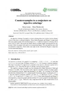
As mentioned in Chapter 3, we expect that our theoretical results give an accurate lower bound on the stabilization time of the coloring algorithm. Indeed, when considering a complete graph, once a node u has chosen an available color, every other node in the network knows that color (as a neighboring node of u) and thus will not choose it anymore. However, in a non-complete graph, a situation such as illustrated in Figure 4.1 (for distance-1 coloring) may occur and thus, the average stabilization time would be a bit higher than the one in a complete graph, therefore our theoretical analysis only leads to a lower bound. For example, let’s run the algorithm over the graph plotted on Figure 4.1. Every node has to choose a color from 1 to 4 until getting a locally unique color. Node B has two neighbors, A and C. The example shows the colors drawn at each step by each node. As there still exists conflicts at the end of the three steps, the algorithm would not stop yet. But, from theoretical analysis, at the end of the three steps, every urn has been kept aside, so the system should have stabilized. Available colors to B

System execution

Kept aside balls by B

Step 1

A,0

B,0

C,0

D,0

1

2

3

Step 2

A,1

B,1

C,3

D,3

0

2

4

C

Step 3

A,1

B,2

C,2

D,4

0

3

4

A

4

C

Figure 4.1: A possible execution for distance-1 coloring in a synchronous network. In order to evaluate the difference between the analytical lower bound and the simulated stabilization time, we compute by simulation the number of times that two neighboring nodes not originally in mutual conflict have to both choose another color and both get the same color. Results for a distance-1 synchronous scheduling coloring are given in Figure 4.2. As we can see, the greater the color domain size, the more unlikely this case is to appear (almost 0 percent of the cases when the color domain size is quadratic in the maximum degree of the nodes). We also note that, even for a small color domain size (such as twice the maximum degree), this case does not occur very often (less than 18 percent in the worst 12

Proportion of creation of new conflicts over the number of color re-drawing

case). Thus, we can expect that in practice, our analytical result gives a very accurate lower bound on the stabilization time of the coloring protocol. 0.18 ’All but One’ Mode, Max = max degree *2 ’All’ Mode, Max = max degree * 2 ’All but One’ Model, Max = Node degree square ’All’ Mode, Max = Node degree square ’All but One’ Mode, Max = Max degree square ’All’ Mode, Max = max degree square

0.16

0.14

0.12

0.1

0.08

0.06

0.04

0.02

0 500

600

700 800 900 Process Intensity (Number of nodes)

1000

1100

Figure 4.2: Proportion of nodes creating a new conflict over the number of nodes choosing another color. Tables 4.2 and 4.1 compare analytical and simulation results for the Synchronous scheduling in both modes, when using two different color domain sizes |∆|. As expected, theoretical results give tight lower bounds of the simulation outcome.

4.3

Stabilization time.

Figures 4.3 presents the stabilization time for each scheduling hypothesis and both modes when using different sizes of color domain, for a random spatial distribution of the nodes. The most striking results compared to those of [10] is that the stabilization time is much lower than expected. From the results of [10], the stabilization time is at least linear in |∆| (being upper bounded by a constant when δ is also a constant). In contrast, our simulation results show a sub-linear (in |∆|) stabilization time, since considering |∆| = 2 × maxp∈V |Np | vs. |∆| = maxp∈V |Np |2 merely divides by two the stabilization time. Also, doubling the degree of the nodes (when the network grows from 500 nodes to 1100 nodes) does not double the stabilization time. Especially, with the synchronous and probabilistic distributed schedulers, the stabilization time remains upper bounded by a constant.

13

4 neighbors all but one all 2 ∗ M ax M ax2 2 ∗ M ax M ax2 Theory Simulation Theory Simulation Theory Simulation Theory Simulation 1.88 1.89 1.51 1.64 2.14 2.14 1.56 1.61 8 neighbors all but one all 2 ∗ M ax M ax2 2 ∗ M ax M ax2 Theory Simulation Theory Simulation Theory Simulation Theory Simulation 1.51 1.56 1.14 1.22 1.56 1.67 1.15 1.21

Table 4.1: Theory and simulations results for the stabilization time for synchronous distance1 coloring with |∆| = (maxp∈V |Np |)2 ) and |∆| = 2 × (maxp∈V |Np |) in a grid. 500 nodes 15.7

600 nodes 18.8

Theory Simulation

2.35 2.78

2.40 2.91

Theory Simulation

2.83 3.25

2.91 3.31

Mean degree

700 nodes 800 nodes 22.0 25.1 all but one 2.44 2.50 2.87 2.94 all 2.94 2.95 3.29 3.28

900 nodes 28.3

1000 nodes 31.4

2.53 2.99

2.56 2.97

3.05 3.42

3.08 3.41

Table 4.2: Theory and simulations results for the stabilization time for synchronous distance1 coloring with |∆| = 2 × (maxp∈V |Np |) random geometry topology. In all cases, whatever the coloring distance and ∆, we can note that the behavior of both probabilistic schedulers is similar. With the probabilistic scheduling hypothesis, in order to stabilize, the scheduler has to choose a node in conflict. In the all but one mode, only one node per pair of conflicting nodes actually chooses another color. The probabilistic schedulers thus have less chance to elect a conflicting node in the all but one mode than in the all mode (almost half chances less). Therefore, with the all mode, these probabilistic schedulings achieve better stabilization time (almost half time) than with the all mode. In the synchronous mode, at each step, every node acts. As in the all but one mode, in any pair of conflicting nodes, already one of those nodes has a stable color, so the stabilization time is lower than in the all mode. Note that for sensor networks, nodes are rarely tightly synchronized, so that the most realistic model is the distributed probabilistic scheduler, so the all mode is to be preferred in this context. Results for distance-2 coloring are not plotted here but are similar to distance-1 coloring results in shape and lead to the same conclusions.

14

4.4

Influence of the size of the color domain.

Since the most realistic model for sensor networks is the distributed probabilistic one, Figures 4.4(a) and 4.4(b) plot the stabilization time for the distance-1 coloring algorithm with all mode as well as the height of the induced DAG, using different sizes of color domain. Nevertheless, results for the DAG height are similar whatever the coloring hypothesis. Results clearly show that a higher domain size |∆| induces a lower stabilization time and a higher DAG. There is thus a trade-off between these two characteristics depending of the application that will use the coloring. However, and although theoretical results show that the DAG height can be up to ∆ − 1, simulation results show that the actual height is in fact much lower, and most certainly sub-linear in ∆. Results for distance-2 coloring are not plotted here but are similar to distance-1 coloring results in shape and lead to the same conclusions.

15

7.5 Synchronous scheduling, ’All but One’ Mode Synchronous Scheduling, ’All’ Mode Distributed Probabilistic Scheduling, ’All but One’ Mode Distributed Probabilistic Scheduling, ’All’ Mode Central Probabilistic Scheduling, ’All but One’ Mode Central Probabilistic Scheduling, ’All’ Mode

Stabilization time (Number of steps before stabilization)

7

6.5

6

5.5

5

4.5

4

3.5

3 500

600

700 800 900 Process Intensity (Number of nodes)

1000

1100

(a) |∆| = 2 × maxp∈V |Np |

4.5 Synchronous Scheduling, ’All but One’ Mode Synchronous Scheduling, ’All’ Mode Distributed Probabilistic Scheduling, ’All but One’ Mode Distributed Probabilistic Scheduling, ’All’ Mode Central Probabilistic Scheduling, ’All but one’ Mode Central Probabilistic Scheduling, ’All’ Mode

3

Stabilization Time (Number of steps before stabilization)

Stabilization Time (Number of steps before stabilization)

3.5

2.5

2

1.5

1 500

600

700 800 900 Process Intensity (Number of nodes)

(b) |∆| = maxp∈V |Np |

1000

1100

2

Synchronous Scheduling, ’All but One’ Mode Synchronous Scheduling, ’All’ Mode Distributed Probabilistic Scheduling, ’All but One’ Mode Distributed Probabilistic Scheduling, ’All’ Mode Central Probabilistic Scheduling, ’All but one’ Mode Central Probabilistic Scheduling, ’All’ Mode

4

3.5

3

2.5

2

1.5

1 500

600

700 800 900 Process Intensity (Number of nodes)

1000

2

(c) |∆| = |Np |

Figure 4.3: Stabilization time of the distance-1 coloring process for different modes and scheduling hypothesis over a geometric node distribution with different sizes of color domain.

16

1100

Stabilization Time (Number of steps before stabilization)

3 Max = 2 * Max degree Max = Node degree * node degree Max = Max Degree * Max Degree

2.8

2.6

2.4

2.2

2

1.8

1.6

1.4

1.2 500

600

700 800 900 Process Intensity (Number of nodes)

1000

1100

(a) Stabilization time 2 max = 2 * max degree, ’All but One’ Mode max = 2 * max degree, ’All’ Mode max = max degree square, ’All but One’ Mode max = max degree square, ’All’ Mode max = node degree square, ’All but one’ Mode max = node degree square, ’All’ Mode

1.95

DAG length

1.9

1.85

1.8

1.75

1.7 500

600

700 800 900 Process Intensity (Number of nodes)

1000

1100

(b) DAG height

Figure 4.4: Influence of the color domain size on the stabilization time and the DAG height.

17

Chapter 5 Concluding remarks Distance-k coloring is a useful mechanism for sensor networks. In [10], distance-3 coloring was used to construct a TDMA schedule, and in [12], distance-2 coloring permitted to expedite density based cluster construction. Further applications could be derived, e.g. distance-k maximal independent set construction, by having nodes that have locally minimal color in their k neighborhood be part of the independent set, and remaining nodes that do not see distance-k neighbors (with lower color) in the independent set join the independent set. In this paper, we show analytically and by simulation that the stabilization time of such coloring protocols is low. Nevertheless, we did not take into account the delay induced by the communication at distance-k of the color of each node, reducing it to a given constant. Further studies are needed to get a more realistic bound that takes into account the probabilistic nature of the MAC layer of ad hoc and sensor networks. Indeed, as k grows, the size of the messages get longer (in the order of δ k−1 , since a node needs to communication information about its neighborhood at distance k − 1 to each of its neighbors), so the probability that collisions occurs between neighboring grows, and the delay increases.

18

Bibliography [1] G. Chelius, E. Fleury, B. Sericola, and L. Toutain. On the nap protocol. Technical Report To appear, INRIA, 2005. [2] E. Dijkstra. Self stabilizing systems in spite of distributed control. Communications of the ACM, 17:643–644, 1974. [3] S. Dolev. Self-Stabilization. The MIT Press, 2000. [4] M. Eisen. Introduction to Mathematical Probability Theory. Prentice Hall, Englewood Cliffs, 1969. [5] FRAGILE. Failure Resilience and Application Guaranteed Integrity in Large-scale Enviroments. http://www.lri.fr/∼fragile/. [6] S. Ghosh and Mehmet Hakan Karaata. A self-stabilizing algorithm for coloring planar graphs. Distributed Computing, pages 7:55–59, 1993. [7] M. Gradinariu and C. Johnen. Self-stabilizing neighborhood unique naming under unfair scheduler. In Euro-Par 2001, volume 2150 of LNCS, pages 458–465. Springer, 2001. [8] M. Gradinariu and S. Tixeuil. Self-stabilizing vertex coloring of arbitrary graphs. OPODIS’2000, pages 55–70, Paris, France, December 2000.

In

[9] S. Hedetniemi, D. Jacobs, and P. Srimani. Linear time self-stabilizing colorings. Inf. Process. Lett., 87(5):251–255, 2003. [10] T. Herman and S. Tixeuil. A distributed tdma slot assignment algorithm for wireless sensor networks. In AlgoSensors’2004, number 3121 in LNCS, pages 45–58, Turku, Finland, July 2004. [11] N Lynch. Distributed algorithms. Morgan Kaufmann, 1996. [12] N. Mitton, E. Fleury, I. Gu´erin-Lassous, and S. Tixeuil. Self-stabilization in self-organized wireless multihop networks. In Proceedings of WWAN’05. IEEE Press, 2005. [13] Mikhail Nesterenko and Anish Arora. Tolerance to unbounded byzantine faults. In IEEE SRDS 2002, pages 22–, 2002. [14] Raida Perlman. Interconnections: Bridges, Routers, Switches, and Internetworking Protocols. Addison-Wesley Longman, 2000.

19

[15] S. Shukla, D. Rosenkrantz, and S. Ravi. Observations on self-stabilizing graph algorithms for anonymous networks. In Proceedings of the Second Workshop on Self-stabilizing Systems (WSS’95), pages 7.1–7.15, 1995. [16] S. Sur and P. Srimani. A self-stabilizing algorithm for coloring bipartite graphs. Information Sciences, 69:219–227, 1993.

20