ON FIRST-PASSAGE PROBLEMS FOR. ASYMMETRIC DIFFUSIONS. MARIO ABUNDO. Dipartimento di Matematica. Universit`a Tor Vergata. 00133 Roma, Italy ...
ON FIRST-PASSAGE PROBLEMS FOR ASYMMETRIC DIFFUSIONS
MARIO ABUNDO Dipartimento di Matematica Universit` a Tor Vergata 00133 Roma, Italy.
1
X(t) a temporally homogeneous, one-dimensional diffusion process over I = (−b, a), (a, b > 0) which is the solution of the SDE: dX(t) = µ(X(t))dt + σ(X(t))dBt , X(0) = x ∈ I Bt a standard Brownian motion (BM). • µ(x) = µ+ (x) if x > 0, µ(x) = µ− (x) if x < 0 • σ(x) = σ + (x) if x > 0, σ(x) = σ − (x) if x < 0 • µ± (x) and σ ± (x) regular enough functions. X(t) turns out to be a sign-dependent diffusion. • µ(x) and σ(x) are not assigned at x = 0. We can take µ± (x) and σ ± (x) as parametric functions of the state x (e.g. polynomials in the unknown x, with coefficients θi± , i = 0, . . . , n and ηj± , j = 0, . . . , m, respectively). We suppose that, when X(t) hits 0, it goes right to the position δ > 0 with probability p > 0 and left to the position −δ with probability q = 1−p : the process is reflected at zero rightward or leftward. As a generalization, the infinitesimal coefficients may change when the process X(t) crosses any given barrier, not necessarily the origin.
2
Applications in Mathematical Finance
˜ Suppose that X(t) is the price of a stock or a commodity, such as gold or oil, or an interest rate, at time t. ˜ In practice, when X(t) reaches a certain threshold S, it may become much more volatile (or much less volatile). The same thing occurs for the drift term. Thus, volatility and drift may undergo a sharp ˜ variation, when X(t) crosses the threshold S. ˜ If X(t) is asymmetric diffusion at S : ˜ ˜ ˜ ˜ dX(t) =µ ˜(X(t))dt +σ ˜ (X(t))dB t , X(0) = x
•µ ˜(x) = µ ˜+ (x) if x > S, µ ˜(x) = µ ˜− (x) if x < S •σ ˜ (x) = σ ˜ + (x) if x > S, σ ˜ (x) = σ ˜ − (x) if x < S ˜ Setting X(t) = X(t) − S, the process X(t) turns out to be asymmetric diffusion at zero, with infinitesimal parameters µ(x), σ(x), changing when X(t) crosses the origin. dX(t) = µ(X(t))dt + σ(X(t))dBt where µ(x) = µ ˜(x + S), σ(x) = σ ˜ (x + S)
Special case: µ± and σ ± linear functions of x (that is µ± (x) = θ1± x + θ0± , σ ± (x) = η1± x + η0± ) it includes: • the asymmetric BM with drift µ+ and diffusion coefficient σ + when X(t) > 0, and µ− and σ − when X(t) < 0 (i.e. θ1± = 0, θ0± = µ± , η1± = 0, η0± = σ ± ) • the asymmetric version of the Ornstein-Ulenbeck (O-U) process, or Vasicek model dX(t) = −µX(t)dt + σdBt with parameters µ± < 0 and σ ± (i.e. θ1± = µ± , θ0± = 0, η1± = 0, η0± = σ ± ). (indeed the usual Vasicek model solves dX(t) = −µ(X(t) − α)dt + σdBt , which is reduced to the simpler version, here considered, set˜ ting X(t) = X(t) − α) • the asymmetric version of the Cox-Ingersoll-Ross (CIR) pro√ cess dX(t) = −µ(X(t) − α)dt + σ X(t)dBt ; note that, for special values of the parameters the CIR process reduces to the quare of O-U: if αµ = σ 2 /4, then X(t) = Y 2 (t), where dY (t) = −(µY (t)/2)dt + (σ/2)dBt √ If O-U Y (t) is asymmetric at S, then X(t) turns out to be asymmetric at S.
drift b + diffu σ +
X (t)
x=S
drift b − diffu σ − X(0)
time
TWO-DIMENSIONAL SITUATION
ONE-DIMENSIONAL SITUATION
MEAN VELOCITY FIELD v(x) v− at the left hand side w.r.t. the barrier S v+ at the right hand side w.r.t. the barrier S
OUTLINE OF THE TALK
1. THE FIRST-PASSAGE TIME FOR ASYMMETRIC DIFFUSIONS 2. NUMERICAL RESULTS
4
1. THE FIRST-PASSAGE TIME FOR ASYMMETRIC DIFFUSIONS For a, b > 0, let τ (δ, x) be the first-exit time of X(t) from the interval I = (−b, a), when starting at x ∈ I i.e.: τ (δ, x) = τ (x) = inf{t > 0 : X(t) = a or X(t) = −b|X(0) = x} The probabilities of exit at left π− (x) = P (X(τ (x)) = −b|X(0) = x) and at right π+ (x) = 1 − πP (X(τ (x)) = a|X(0) = x) For ordinary diffusions (i.e. µ± (x) = µ(x), σ ± (x) = σ(x) and no reflection at zero), explicit formulae are available to calculate E(τ (x)) and π ± (x), x ∈ (−b, a), in the case when P (τ (x) < ∞) = 1. Lefebvre [2006] studied the process X(t) = µt + σBt (i.e. asymmetric Brownian motion with drift) where µ and σ depend on the sign of X(t), and jumps of amplitude ±δ occur with probability p and 1 − p when X(t) = 0. He found explicit formulae for π ± (x) and for the moment generating function of τ (x), in the limit δ → 0+ . OUR AIM: to find closed analytical expressions for the exit probabilities and the mean exit time of an asymmetric diffusion (continuation of talk given at EUROCAST 2007). 5
In alternative to those heavy calculations, we will also propose a method (see also Abundo, Eurocast 2007, LNCS) to find approximate estimates.
6
• X(t) asymmetric diffusion over I = (−b, a) : dX(t) = µ(X(t))dt + σ(X(t))dBt , X(0) = x ∈ I � + µ (X(t)) if X(t) > 0 • µ(X(t)) = µ− (X(t)) if X(t) < 0 � + σ (X(t)) if X(t) > 0 • σ(X(t)) = σ − (X(t)) if X(t) < 0 • note that µ(0) and σ(0) are not assigned. When X(t) hits the origin, it goes right to the position δ > 0 with probability p > 0 and left to the position −δ with probability q = 1 − p. . Denote by X + (t) the diffusion on I + = (0, a) having infinitesimal coefficients µ+ (·) and σ + (·), and by X − (t) the diffu. sion on I − = (−b, 0) having infinitesimal coefficients µ− (·) and σ − (·). Assume the usual conditions for existence and uniqueness of solutions. 1 ± (σ (x))2 f 00 (x) + µ± (x)f 0 (x), f ∈ C 2 (I ± ) 2 the infinitesimal generators associated to the two diffusions in the positive and the negative half part of the interval I, acting on C 2 functions (I + = (0, a), I − = (−b, 0)). • L± f (x) =
Assume that −b and 0 are attainable boundaries for the process X − (t), and 0 and a are attainable boundaries for . the process X + (t). Finally, suppose that τ (δ, x) = inf{t > 0 : X(t) ∈ / (−b, a)|X(0) = x ∈ I} is finite with probability one, for any x ∈ I. 7
Set:
. • π + (x) = π + (δ, x) = P (X(τ (x)) = a|X(0) = x) the probability that X(t) hits a before −b from x ∈ (−b, a) . • π − (x) = π − (δ, x) = P (X(τ (x)) = −b|X(0) = x) = 1 − π + (x) the probability that X(t) hits −b before a from x ∈ (−b, a) To simplify notations, we will drop the dependence of τ and π + on δ. We will find explicit formulae for the mean exit time from I and the exit probability through the right end a, in the limit δ → 0+ : . . E(τ (x))∗ = lim+ E(τ (x)) and π + (x)∗ = lim+ π + (x) δ→0
δ→0
For ordinary diffusions (i.e. µ± (x) = µ(x), σ ± (x) = σ(x) and no jump at zero), explicit formulae are available to calculate E(τ (x)), π ± (x), x ∈ (−b, a). The infinitesimal generator of X(t) becomes Lf (x) =
1 2 σ (x)f 00 (x) + µ(x)f 0 (x), x ∈ I, 2
and the mean exit time E(τ (x)) from the interval I is the solution of: Lv(x) = −1, x ∈ I; v(−b) = v(a) = 0 8
(1)
while π± (x) solves the equation: Lπ± (x) = 0, x ∈ I π (a) = 1, π+ (−b) = 0 + (π− (a) = 0, π− (−b) = 1)
(2)
Moreover, if τ± (x) is the exit time of X from I with the condition that exit has occurred at the right (respectively the left) of I : T± (x) E(τ± (x)) = π± (x) where T± (x) is the solution of the problem: � Lz(x) = −π± (x) , x ∈ I z(−b) = z(a) = 0
(3)
and it results E(τ (x)) = E(τ− (x))π− (x) + E(τ+ (x))π+ (x)
• 1.1 THE EXIT PROBABILITY THROUGH THE RIGHT END OF I, IN THE LIMIT δ → 0+ We will find an explicit formula for π + (x)∗ by calculating the limit of π + (x), as δ → 0+ . Set: � Z φ+ (x) = exp −
2µ+ (z) dz (σ + (z))2
x
2µ− (z) dz (σ − (z))2
0
� Z φ− (x) = exp −
−b
9
�
x
�
and
Z
Z
x
+
ψ (x) =
+
−
x
φ (z)dz, ψ (x) = 0
φ− (z)dz
−b
Then: . P {X(t) hits a before 0 from x ∈ (0, a)} = ψ + (x) . + = π(0,a) (x) = + ψ (a) . and P {X(t) hits 0 before −b from x ∈ (−b, 0)} = ψ − (x) . + = π(−b,0) (x) = − ψ (0) Proposition 1 (Abundo, 2008) Under the assumptions and notations above, it holds: ∗
π + (x) = lim π + (x) = + δ→0
=
+ � ψ (x) + + 1− ψ (a)
ψ + (x) ψ + (a)
� p
p ψ − (0) ψ + (a)φ− (0)
ψ − (0)+q
p ψ − (x) p ψ − (0)+q ψ + (a)φ− (0)
if 0 ≤ x ≤ a if −b ≤ x ≤ 0
10
Example 1 (asymmetric Brownian motion with drift (Lefebvre, 2006)) X(t) = µt + σBt , � + � + µ if x(t) > 0 σ if X(t) > 0 µ= , σ= − − µ if X(t) < 0 σ if X(t) < 0 (i) 0 ≤ x ≤ a a) µ± 6= 0 ∗
+
π (x) =
+ π(0,a) (x)
� + 1−
+ π(0,a) (x)
� ·
−
pβ + (1 − ebβ ) · + pβ (1 − ebβ − ) + qβ − (e−aβ + − 1) where + π(0,a) (x)
=
−xβ + 1−e−aβ+
if µ+ 6= 0
x
if µ+ = 0
1−e a
,
β
±
2µ± = ± 2 (σ )
b) µ+ = µ− = 0 x � x � pb π (x) = + 1 − a a pb + qa +
∗
(ii) −b ≤ x ≤ 0 ∗
+ π + (x) = π(−b,0) (x)π + (0)∗ ,
where
( + π(−b,0) (x)
=
−
e−xβ −ebβ 1−ebβ − b+x b
11
−
if µ− 6= 0 if µ− = 0
Remark If a = b, p = q = 1/2, µ± = 0, and σ ± = 1, we obtain ∗ π + (x) = x+a 2a , x ∈ (−a, a) that is the expression of the exit probability through the right end a of the ordinary BM starting from x ∈ (−a, a), (i.e. the solution of 1 00 w (x) = 0; w(−a) = 0, w(a) = 1) 2 Example 2 (asymmetric O-U process) (µ± > 0 and σ ± > 0) dX(t) = −µX(t)dt + σdBt where � µ=
µ+ µ−
if X(t) > 0 , σ= if X(t) < 0
�
σ+ σ−
if X(t) > 0 if X(t) < 0
We get: for 0 ≤ x ≤ a ∗
+ + π + (x) = π(0,a) (x) + (1 − π(0,a) (x))·
p
R0
e{s −b
2
·µ− /(σ − )2 }
ds
· R0 Ra p −b e{s2 ·µ− /(σ− )2 }) ds + q 0 e{s2 ·µ+ /(σ+ )2 } ds where
R x {s2 ·µ+ /(σ+ )2 } e ds + π(0,a) (x) = R0a {s2 ·µ+ /(σ+ )2 } e ds 0
for −b ≤ x ≤ 0 ∗
π + (x) =
p
R0 −b
p
Rx
e{s −b
2
·µ− /(σ − )2 })
e{s2 ·µ− /(σ− )2 } ds + q 12
Ra 0
ds
e{s2 ·µ+ /(σ+ )2 } ds
• 1.2 THE MEAN EXIT TIME FROM I IN THE LIMIT δ → 0+ We will find an explicit formula for . E(τ (x))∗ = lim E(τ (x)) δ→0+
For α = 0, or α = a, set: . θ˜α (x) =
Z
x
ξ˜α (t)dt
0
. ξ˜α (x) = φ+ (x)
Z
x
2fα (s)[(σ + (s))2 (s)φ+ (s)]−1 ds
0
and . − . + + f0 (x) = π(0,a) (x) = 1 − π(0,a) (x), fa (x) = π(0,a) (x) For β = −b, or β = 0, set: . ηˆβ (x) =
Z
x
ζˆβ (t)dt,
−b
. ζˆβ (x) = φ− (x)
Z
x
2gβ (s)[(σ − (s))2 (s)φ− (s)]−1 ds
−b
and . + . − + g0 (x) = π(−b,0) (x), g−b (x) = π(−b,0) (x) = 1 − π(−b,0) (x) Then, it holds: 13
Proposition 2 (Abundo, 2008) ∗
E(τ (x)) = lim E(τ (x)) = δ→0+
=
+ + ˜a (a) ψ + (x) − θ˜a (x) + θ˜0 (a) ψ + (x) − θ˜0 (x)+ θ ψ (a) � ψ (a) � + + 1 − ψ + (x) E(τ (0))∗ if x ∈ (0, a) ψ (a) ψ − (x) ψ − (x) η ˆ (0) − η ˆ (x) + η ˆ (0) ˆ0 (x)+ −b −b 0 ψ − (0) ψ − (0) − η ψ− (x) + ψ− (0) E(τ (0))∗ if x ∈ (−b, 0)
where �
p qφ− (0) ∗ E(τ (0)) = lim E(τ (0)) = + − ψ + (a) ψ (0) δ→0+ n × �Z + qφ− (0)
0
−b
�−1 ×
p (θ˜0 (a) + θ˜a (a))+ ψ + (a)
� ηˆ0 (0) + ηˆ−b (0) o 2 ds − (σ − (s))2 φ− (s) ψ − (0)
REMARK If µ± = 0, σ ± = 1 (i.e. for ordinary BM), after simple but tedious calculations we obtain: ∗
E(τ (0)) = ab
ap + bq bp + aq
and � ∗
E(τ (x)) =
−x2 + xa (a2 − E(τ (0))∗ ) + E(τ (0))∗ −x2 + xb (E(τ (0))∗ − b2 ) + E(τ (0))∗ 14
if x ∈ (0, a) if x ∈ (−b, 0)
Moreover, if p = q or a = b, it follows E(τ (0))∗ = ab and so E(τ (x))∗ = −x2 +x(a−b)+ab, x ∈ (−b, a) that is the expression of the mean exit time of ordinary BM from the interval (−b, a), when starting at x ∈ (−b, a) (i.e. the solution of 1 00 2 w (x)
= −1; w(−b) = w(a) = 0).
As one can see, Proposition 2.1 and 2.2 provide explicit formulae, but long and tedious computations are needed in general to obtain every quantity, if one does not calculate numerically the integrals. Then, we will introduce a method to estimate numerically π + (x)∗ and E(τ (x))∗ , avoiding the direct use of the above formulae.
• 1.3 THE MOMENT GENERATING FUNCTION OF τ (x) IN THE LIMIT δ → 0+ For a general asymmetric diffusion, it is impossible to obtain an exact analytical formula for the Laplace transform of τ (x) in the limit δ → 0+ , i.e h i∗ h i . −λτ (x)) −λτ (x)) M (x) = E e = lim+ E e , λ>0 ∗
δ→0
(for the asymmetric BM with drift, the explicit form of � −λτ (x)) �∗ E e was found in [Lefebvre, 2006]).
15
However the following representation holds for x ∈ (0, a) : pMδ,a + qN−δ,−b M (x)∗ = Mx,a + Mx,0 lim+ δ→0 1 − pMδ,0 − qN−δ,0 The representation for M (x)∗ when x ∈ (−b, 0) is obtained by replacing Mx,a by Nx,−b and Mx,0 by Nx,0 . Here: • Mx,a , as a function of x ∈ [0, a], satisfies the equation L+ z(x) = λz(x), and it increases from 0 to 1 in the interval [0, a]; • Mx,0 , as a function of x ∈ [0, a], satisfies the equation L+ z(x) = λz(x) and it decreases from 1 to 0 in the interval [0, a]; • Nx,−b , as a function of x ∈ [−b, 0], satisfies the equation L− z(x) = λz(x) and it decreases from 1 to 0 in the interval [−b, 0]; • Nx,0 , as a function of x ∈ [−b, 0], satisfies the equation L− z(x) = λz(x) and it increases from 0 to 1 in the interval [−b, 0]. Although the above equations are linear ODEs of the second order, their coefficients (except in the case of BM with drift) are functions of x, so in general their solutions cannot be found in an analytical way. Therefore, to obtain M (x)∗ one has to solve them numerically.
16
THE APPROXIMATE ESTIMATES The existence and uniqueness of the strong solution of the SDE on the entire interval I require µ(x) to be Lipschtiz continuous and σ(x) to be Holder continuous. Unfortunately, µ(x) and σ(x) may be not continuous at x = 0, since µ(0+ ) = µ+ (0) is allowed to be different from µ(0− ) = µ− (0), and in analogous way σ(0+ ) = σ + (0) can be different from σ(0− ) = σ − (0). Consider, e.g. the drift µ(x), and suppose that µ(x) = θ1 x + θ0 , where � + θi if x > 0 θi = − θi if x < 0 Then, µ(0+ ) = θ0+ and µ(0− ) = θ0− ; thus, through the origin µ(·) passes from the value θ0− to θ0+ , requiring a regularization in order to make µ(x) continuous at x = 0. Suppose e.g. θ0− < θ0+ ; we can interpolate θ0 in a neighbor of the origin by means of a continuous piecewise-linear function, in the following way. Take a small h > 0 and α ∈ (θ0− , θ0+ ) and set: − if x < x∗ θ0 + θ0 = α + x(θ0 −α) if x∗ ≤ x ≤ h h + θ0 if x > h . where x∗ = −h(α − θ0− )/(θ0+ − α). With these modifications, µ(x) = θ1 x + θ0 becomes continuous at x = 0, since µ+ (0) = µ− (0). However, the discontinuity in µ(x) appears if one let h go to zero. If one seeks only a weak solution to the SDE, it is not necessary to consider any regularization of the coefficients. 17
The value α above is responsible of the asymmetry between the values of the drift at the left and at the right of the origin (if α = (θ0+ − θ0− )/2 we have perfect symmetry). Suppose e.g. µ± (x) = θ0± ∀x (θ0+ > θ0− ) and σ(x) = const.; then the parameter α takes into account the mean velocity of the α−θ − process X(t) near zero. If we set r = θ+ −θ0− , for r > 1/2 0 0 the process moves to the right more quickly in the average when X(t) = 0+ than when X(t) = 0− , and the viceversa holds for r < 1/2, while r = 1/2 represents the case when the mean velocity of the process is approximately the same in the left and right neighbor of the origin.
The approximation argument: First, suppose that X(t) is an ordinary diffusion (without reflection at the origin, no jump when X(t) = 0), with regular infinitesimal coefficients, and set µ(0) = µ+ (0), σ(0) = σ + (0). Then, for h → 0 : X(t + h) = X(t) + µ(X(t))h + σ(X(t))∆Bh + o(h)
(i)
So, recalling the meaning of the drift µ(x) and the infinitesimal variance σ 2 (x), it holds: E[X(t + h) − X(t)|X(t) = x] = µ(x)h + o(h)
(ii)
E[(X(t + h) − X(t))2 |X(t) = x] = σ 2 (x)h + o(h)
(iii)
and
18
Now, we introduce the reflection at 0, by allowing X(t) to make a jump ∆ ∈ {−δ, δ} when it hits 0 (with P (∆ = δ) = p and P (∆ = −δ) = 1 − p); in place of (i) we obtain, as h → 0 : X(t + h) = X(t) + µ(X(t))h + σ(X(t))∆Bh + ∆ · 1{0} (X(t)) + o(h) (i0 ) where 1{0} (x) = 1 if x = 0, and 0 otherwise. Moreover, since the mean of the random variable ∆ is (2p − 1)δ and its variance is 4p(1 − p)δ 2 , we obtain, on the analogy of (ii), (iii): E[X(t+h)−X(t)|X(t) = x] = µ(x)h+(2p−1)δ·1{0} (x)+o(h) (ii0 ) and + V
E[(X(t+h)−X(t))2 |X(t) = x] = σ 2 (x)h4p(1−p)δ 2 ·1{0} (x)+o(h) . (iii0 ) If we choose δ = h, in the approximation h ≈ 0, we get that the asymmetric diffusion X(t) with reflection at the origin b can be approximated by a diffusion X(t) without reflection at zero, having infinitesimal parameters µ ˆ(x) = µ(x) + (2p − 1) · 1{0} (x), and σ ˆ 2 (x) = σ 2 (x) (note that the term 4p(1 − p)δ 2 · 1{0} (x) is o(h2 )). Alternatively, we can consider the jump-diffusion process (with jumps allowed only when X(t) = 0), with generator . L1 f = Lf + Lj f where the additional “jump” part is given by Lj f = pf (δ) + (1 − p)f (−δ) − f (0) 19
i.e. p[f (δ) − f (0)] + (1 − p)[f (−δ) − f (0)]. At the first order, as δ → 0, the last quantity equals pf 0 (0)δ+ (1 − p)f 0 (0)(−δ) = δ(2p − 1)f 0 (0) which agrees with the expression already found for µ ˆ(x).
20
• 2. NUMERICAL RESULTS The above arguments show that approximations to π ± (x), E(τ (x)) and E(τ ± (x)) for δ ≈ 0, can be obtained by calcub (x)) and E(τ b ± (x)) lating the analogous quantities π b± (x), E(τ b concerning the ordinay diffusion X(t). We have calculated them, by using the classical results for ordinary diffusions.(equations. (1), (2), (3)) b In practice, the drift of X(t) has been taken equal to that of X(t), except in a small neighbor of the origin (−ε, ε), where b the drift of X(t) was augmented of the quantity (2p − 1). Numerical computations were carried on by running a FORTRAN program written by us, with ε = 0.01 . For asymmetric BM with drift, we have compared our apb (x)) with the exact values π + (x)∗ proximations π b+ (x) and E(τ and E(τ (x))∗ , obtaining a satisfactory agreement. We have also considered the ordinary O-U process, i.e. the solution of dX(t) = −µX(t)dt + σdBt and the corresponding process with asymmetric reflection at the origin; for the latter process we have estimated the exit probability through the right end of the interval I and the mean exit time from I, when starting at x ∈ I.
21
EXACT
APPROXIMATION
Figure 1 exit probability at right, as a function of x ∈ (−b,a), for the asymmetric BM with drift; comparison between the exact value π+(x) (above) and its approximation π+(x) (below). The values of the parameters are a = 1= − b, µ+ = 2, µ− = 1, σ = σ+ = σ− = 1, and p =0.8. Although π+(x) presents some oscillations for x ∈ (0, 0.2), the agreement between the two curves is excellent.
Figure 2 Comparison among different estimates of π+ (x), as a function of x ∈ (− b, a), for the asymmetric BM with drift, with a = 1 = − b, µ+ = 2, µ− = 1, σ = σ+ = σ− = 1, and p = 0.8. exact value π+ (x) (blue line); estimate π+ (x) (green line); estimate of π+ (x) obtained by regularization of drift in the asymmetric case, r = 0.8 (light-blue line), and in the symmetric case, r = 0.5 (red line)
Figure 3 Comparison among different estimates of E (τ (x)) , as a function of x ∈ (− b, a), for the asymmetric BM with drift, with a = 1 = − b, µ+ = 2, µ− = 1, σ = σ+ = σ− = 1. Estimate of E (τ (x)) obtained by regularization of drift in the symmetric case, r =0.5 (red line) and in the asymmetric case, r = 0.8 (light-blue line); exact value E (τ (x)) for p = 0.8 (blue line); its approximation E (τ (x)) for p = 0.8 (green line) The agreement between the blue and green line is excellent.
Figure 4 Comparison among different estimates of E (τ+(x)) , as a function of x ∈ (− b, a), for the asymmetric BM with drift, with a = 1 = − b, µ+ = 2, µ− = 1, σ = σ+ = σ− = 1. Estimate of E (τ+(x)) obtained by regularization of drift in the symmetric case, r =0.5 (green line) and in the asymmetric case, r = 0.8 (light-blue line); its approximation E (τ (x)) for p = 0.8 (blue line)
Figure 5 Comparison among different estimates of π+ (x), as a function of x ∈ (− b, a), for the asymmetric O-U process which is the solution of dX (t) = − µ X (t) dt + σ dBt, with a = 1 = − b, µ+ = 2, µ− = 1, σ = σ+ = σ− = 1. Exact formulae for π+ (x) are not available. Estimate π+ (x) (green line) for p = 0.8; estimate of π+ (x) obtained by regularization of µ in the asymmetric case, r = 0.8 (blue line). The green line cannot be distinguished from the curve of the exact value of the exit probability, analytically calculated by means of the explicit formula.
Figure 6 Comparison among different estimates of E (τ(x)), as a function of x ∈ (− b, a), for the asymmetric O-U process which is the solution of dX (t) = − µ X (t) dt + σ dBt, with a = 1 = − b, µ+ = 2, µ− = 1, σ = σ+ = σ− = 1. Exact formulae for E (τ(x)) are not available. Estimate E (τ(x)) for p = 0.8 (green line); estimate of E (τ(x)) obtained by regularization of µ in the asymmetric case, r = 0.8 (blue line) The green line cannot be distinguished from the curve of the exact mean exit time, analytically calculated by means of the explicit formula.
REMARK Let us consider diffusions obtained from asymmetric Wiener process, by combining a deterministic transformation and a random time–change. Y (t) = σBt an asymmetric Wiener process with zero drift, having jumps of size ±δ when hitting zero and σ = σ + when Y (t) > 0, σ = σ − , otherwise. (i) X(t) conjugated to Y (t) via an increasing function f, with f (0) = 0, that is f (X(t)) = σBt . Then: n o τ (x) = inf t > 0 : X(t) = −b or X(t) = a|X(0) = x ∈ (−b, a) = n o = inf t > 0 : f (X(t)) = f (−b) or f (X(t)) = f (a)|X(0) = x n o − + = inf t > 0 : σ Bt = f (−b) or σ Bt = f (a) B0 = x ¯ where x ¯=
f (x) σ± ,
according to the sign of x ∈ I.
All previously found formulae for π ± (x)∗ and E(τ (x))∗ hold, with f (−b)/σ − and f (a)/σ + in place of −b and a, and with x ¯ in place of x. (ii) For c, d > 0, let Z(t) (with Z(0) = z ∈ (−d, c)) a diffusion in the interval (−d, c) and let u(z) the scale function, i.e. the solution of Lu(z) = 0, z ∈ (−d, c); u(0) = 0, u0 (0) = 1 22
where L is the infinitesimal generator of Z(t). The process u(Z(t)) turns out to be a local martingale. Suppose that its quadratic variation Z ρ(t) =
t
[u0 (X(s))σ(X(s))]2 ds
0
is deterministic. If ρ(∞) = ∞, u(Z(t)) can be written as ˜ such that a time–changed BM, i.e. there exists a BM B ˜ u(Z(t)) = B(ρ(t)). Let us consider the asymmetric diffusion (with jumps of amplitude ±δ at zero) X(t) = σu(Z(t)), where σ = σ + > 0 when Z(t) > 0, σ = σ − > 0, otherwise. Then, if a = σ + u(c) and −b = σ − u(−d), we obtain: n o τ (x) = inf t > 0 : X(t) = −b or X(t) = a |X(0) = x ∈ (−b, a) = n o b a ˜ ˜ ˜ inf t > 0 : B(ρ(t)) = − − or B(ρ(t)) = + |B0 = u(z) ∈ (u(−d), u(c)) σ σ Therefore, it results ρ(τ (x)) = τ˜(u(z)), where n o − ˜ + ˜ ˜ τ˜(y) = inf t > 0 : σ Bt = −b or σ Bt = a |B0 = y ∈ (u(−d), u(c)) ˜ results to be an asymmetric BM with zero (note that σ B drift). Moreover: π + (x) = P (X(τ (x)) = a) = ˜ τ (u(z))) = a) = P (B(˜ ˜ τ (u(z))) = u(c)) = P (σ + B(˜ 23
and E(τ (x)) = E(ρ−1 (˜ τ (u(z)))), so to calculate π + (x)∗ and E(τ (x))∗ , we can use the formulae previously found, with the obvious modifications. (iii) Let X(t) be as in (ii), and suppose now that ρ(t) is not deterministic, but there exist two deterministic, continuous increasing functions α(t) and β(t), with α(0) = β(0) = 0, such that for every t : α(t) ≤ ρ(t) ≤ β(t) Then, by combining the techniques of [Abundo, 2006] and the previous formulae , one can find lower and upper bounds to π + (x)∗ and E(τ (x))∗ . (iv) (Geometrical BM with asymmetry at x = 1) dX(t) = rX(t)dt + σX(t)dBt , X(0) = x0 r and σ positive constant (in the framework of Mathematical Finance, it describes the time evolution of a stock price X). The explicit solution is X(t) = x0 eµt eσBt , where µ = r − σ 2 /2; so X(t) has a log-normal distribution. We introduce asymmetry in the logarithm of X(t) by considering ˜ the asymmetric Wiener process X(t) = ln x0 +µt+σBt , where � µ=
+
µ µ−
˜ if X(t) >0 , σ= ˜ if X(t) 0 ˜ X(t) 1, the first-exit time of X(t) from the interval (β, α) when starting at x is nothing but the first˜ exit time of the asymmetric Wiener process X(t) from the interval (ln β, ln α) when starting at x ˜ = ln x. The probability that X(t) exits from (β, α) through the right end α when starting at x is nothing but the probability that ˜ X(t) exits from (ln β, ln α) through the right end ln α when starting at x ˜ = ln x.
25
REFERENCES - M. Abundo: First-passage problems for asymmetric diffusions and skew-diffusion processes Preprint, 2008. - M. Abundo: On first-passage problems for asymmetric onedimensional diffusions (2007). In: Computer Aided System Theory EUROCAST 2007, IUCTC Universidad de Las Palmas de Gran Canaria, 66-67 - M. Abundo, Limit at zero of the first-passage time density and the inverse problem for one-dimensional diffusions, Stochastic Anal. Appl., 24, 1119-1145 (2006). - I. I. Gihman, A.V. Skorohod, Stochastic differential equations, Springer-Verlag, New York, 1972. - J. M. Harrison and L.A. Shepp, On skew Brownian motion, Ann. Prob. 9 (2), 309–313 (1981). - N. Ikeda and S. Watanabe, Stochastic differential equations and diffusion processes, North-Holland Publishing Company, 1981. - S. Karlin, H.M. Taylor A second course in stochastic processes Academic Press, New York, 1975. - M. Lefebvre First passage problems for asymmetric Wiener processes, J. Appl. Prob. 43, 175–184 (2006). - O. Ovaskainen, S.J. Cornell Biased movement at a boundary and conditional occupancy times for diffusion processes. J. Appl. Prob. 40, 557–580 (2003).
26