On higher order passive scalar structure functions in grid turbulence

PHYSICS OF FLUIDS

VOLUME 16, NUMBER 11

NOVEMBER 2004

On higher order passive scalar structure functions in grid turbulence Armann Gylfason and Zellman Warhafta) Sibley School of Mechanical and Aerospace Engineering, Cornell University, Ithaca, New York 14853

(Received 22 March 2004; accepted 15 July 2004; published online 5 October 2004) The scalar structure function scaling exponent ␨n is experimentally determined for n 艋 10 in decaying, grid-generated wind-tunnel turbulence with a constant mean temperature gradient. The Reynolds number is varied over the range 150艋 R␭ 艋 700 by using static and active grids. The results show that up to n = 10 the scaling exponent does not saturate although saturation is not precluded at higher orders. There appears to be no dependence of ␨n on Reynolds number and the values of ␨n are the same for the transverse (along the gradient) and the longitudinal (streamwise) structure functions. A compilation of previous work shows large variation in ␨n, with a few results indicating saturation and most not. Reasons for the scatter are attributed to convergence problems at high orders, effects of flow or computational domain size causing clipping of large rare fluctuations, and differences in initial and boundary conditions. © 2004 American Institute of Physics. [DOI: 10.1063/1.1790472] For large n, models9,12 suggest that the scaling exponent ␨n, defined as 具⌬␪共r兲n典 ⬃ r␨n, saturates to a constant value due to the existence of the dominant ramp-cliff structures. The rate at which saturation occurs (with increasing n) and the asymptotic value of the scaling exponents are not predicted. Here we describe perhaps the simplest type of scalar experiment; decaying grid turbulence with a passive crossstream temperature gradient.13–17 The gradient breaks the scalar symmetry and causes preferential alignment of the ramp-cliff structures in its direction. Thus odd order structure functions are nonzero in the transverse direction and the derivative skewness is O共1兲.10,15,17 On the other hand, for this flow there is scalar symmetry in the streamwise direction and thus odd order longitudinal structure functions and derivative moments should be zero (which is observed to a high degree, see below). This does not mean that ramps and cliffs do not occur in the x direction; they are present in all directions but are randomly distributed (except in the mean gradient direction where they are preferentially aligned). Snapshots of the fluctuating scalar field with the ramp cliffs are shown in numerical simulations,9,18 and multipoint correlators19,20 provide geometric insight into these structures. Successful theory will have to provide predictions on the way the anomalous scaling exponents vary with structure function order, whether they are the same in the direction of the mean temperature gradient and normal to it, and whether their approach to the asymptotic value is universal or flow dependent. Here we present measurements of these quantities in our simple flow, and compare them with previous experimental15,21–24 and numerical9,25 results.

I. INTRODUCTION

During the 1990s there were significant advances in the understanding of the advection of a passive scalar field in turbulent flows.1,2 Building on the earlier work of Kraichnan,3–5 theoretical6–8 and numerical work9–11 has produced a firm foundation for the understanding of scalar intermittency, anisotropy, and the behavior of higher order structure functions. Central to this work has been the recognition that the statistical properties of the scalar field are decoupled from the velocity field itself. The lack of dependence of the scalar on the velocity field is clearly shown by the existence of intermittency in the scalar in a purely Gaussian (nonintermittent) velocity field,3–5,10 although it is possible that the details of the intermittency structure are determined by the specific nature of the velocity field. Furthermore, contrary to cascade models, the large and small scales of the scalar field are directly coupled: there exist coherent ramp-cliff structures that affect this coupling.1,2 These structures produce large fluctuations, as well as anisotropy, at the small scales. They are inherent to the mixing process and are not reflections of the velocity field itself. The persistent anisotropy and the related intense intermittency of the scalar field is reflected in the strong departure of the higher order structure function (SF) scaling exponents from elementary Kolmogorov–Obukhov–Corrsin (KOC) scaling (e.g., Warhaft2); a departure that is much greater than that of the velocity field in which it is embedded. KOC scaling predicts 具⌬␪共r兲n典 ⬃ rn/3 where ⌬␪共r兲 is the scalar difference over a distance r (which in the present work will be in the streamwise x or the transverse y direction) and n is the structure function order (in this work we only consider positive integers). We are concerned here with inertialconvective subrange intervals, ᐉ␪ 艌 r 艌 ␩␪, where ᐉ␪ and ␩␪ are the scalar integral and dissipation scales, respectively.

II. APPARATUS

Both passive13,14,16,17 and active15 grids have been employed to study scalars in wind tunnels. As in most of these previous experiments, the temperature gradient is in the y direction, normal to the flow 共x兲 direction.16 The mean velocity is constant across the core of the flow and there is no

a)

Telephone: (607) 255-3898; fax: (607) 255-1222; electronic mail: [email protected]

1070-6631/2004/16(11)/4012/8/$22.00

4012

© 2004 American Institute of Physics

Downloaded 05 Oct 2004 to 128.84.137.177. Redistribution subject to AIP license or copyright, see http://pof.aip.org/pof/copyright.jsp

Phys. Fluids, Vol. 16, No. 11, November 2004

On higher order passive scalar structure functions

TABLE I. Flow parameters. The fluctuating parameters were determined at x / M = 36 for the active grid and at x / M = 60 for both passive grids (LG and SG). Passive grid

Active grid

Large grid (LG)

Small grid (SG)

M (cm) U (m/s)

11.4 5.8

10.16 10.8

2.54 10.3

dT / dy (K/m) 具u2典共m2 / s2兲

2.6

4.8

5.3

0.81

0.068

0.044

具␪2典共K2兲 ᐉ (m)

1.04 0.35

0.047 0.09

0.007 0.021

␩ = 共␯3 / ␧兲1/4 (mm) ␭ = 共具u2典 / 具共⳵u / ⳵x兲2典兲1/2 (mm) ␶␩ = 共␯ / ␧兲1/2 (s) ␧ = 15␯具共⳵u / ⳵x兲2典 ⬅ u3 / ᐉ 共m2 / s3兲 ␧␪ = 6␬具共⳵␪ / ⳵x兲2典共m2 / s3兲 Reᐉ = uᐉ / ␯ R␭ = u␭ / ␯

0.20

0.36

0.29

9.4

8.7

4.7

2.7⫻ 10−3 2.05

8.6⫻ 10−3 0.202

5.8⫻ 10−3 0.45

1.25

0.11

0.027

21 400 566

1524 151

290 66

temperature variation in the z direction. With the active grid the mean temperature gradient T共y兲 tends to erode slightly with downstream distance because of the relatively large turbulent integral scale. This causes a weak temperature variation in the x direction.15 For the passive grids T共y兲 remains constant with x, producing the ideal situation with the temperature variation in one direction only, but with a sacrifice in Reynolds number (see Table I). Here we use both active and passive grids in order to study the effects of Reynolds number. We also show that even for the active grid, the odd order moments are negligible in the x (longitudinal) direction, indicating that the longitudinal mean temperature variation is still small compared to the transverse (y direction) gradient and therefore not significantly affecting the scalar field. The temperature gradient was produced by means of differentially heated ribbons, a toaster,16 located in the tunnel plenum, before the honeycomb, screens, and contraction. The temperature fluctuations were produced by the action of the grid on the mean temperature profile. Thus the thermal length scale is set by the grid. The temperature gradient in each measurement was measured at several downstream locations with a thermocouple rake, consisting of 19 thermocouples spaced in the transverse direction of the flow. The passive grids are the same as those employed in Tong and Warhaft17 and Jayesh and Warhaft14 (mesh M = 2.54 cm, small grid, SG, and M = 10.16 cm, large grid, LG), and the active grid 共M = 11.4 cm兲 operated in the random mode, is the same as that used in Mydlarski and Warhaft.15 The reader is referred to those papers for a further description of the flow apparatus and the background velocity fields. All experiments were conducted in our large wind tunnel (91.44⫻ 91.44 cm2 in cross section and 9.1 m long).26 The measurements were done at various downstream locations, 40艋 x / M 艋 100 for the SG, 25艋 x / M 艋 70 for the LG, and 22艋 x / M 艋 62 for the active grid. In Table I typical flow

4013

parameters are listed for a single x / M location for each grid. The temperature fluctuations were measured with singlewire probes connected to dc temperature bridges. Platinum wires, diameter 0.63 ␮m with an etched length of 0.32 mm were used. The velocity fluctuations were measured with TSI 1241 X-array probes connected to Dantec 55M01 constant temperature anemometers. Tungsten wires of 3.05 ␮m diameter were used, with an etched length of 0.6 mm, and the wires were operated at overheat ratio of 1.8. For further information on our temperature and velocity anemometry we refer the reader to Mydlarski and Warhaft.15 Temperature and velocity signals were high and low pass filtered with a Krohn–Hite model 3384 band-pass filter, and digitized with a 12-bit A/D converter. The high-pass filter was in all cases set at 0.01 Hz while the low-pass filter frequency varied between about 2000 and 20 000 Hz for the longitudinal statistics, depending on flow parameters, and the sampling frequency was double the low-pass frequency. For the transverse statistics the sampling frequency was set 400 Hz in all measurements. This low frequency was used to obtain independent data points for the determination of moments. The temperature statistics were obtained from a data series that typically contained about 8 ⫻ 106 – 2 ⫻ 108 data points for longitudinal statistics and around 4 ⫻ 105 data points for transverse statistics. The velocity statistics were obtained from data series containing about 8 ⫻ 106 data points. Taylor’s frozen flow hypothesis was used to obtain data for the longitudinal structure function from a single temperature probe. The transverse structure function was obtained by varying the spacing between two single wire temperature probes.15 III. RESULTS

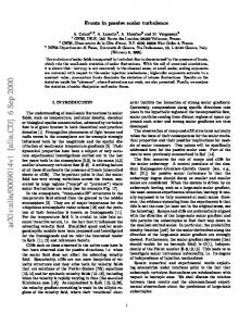
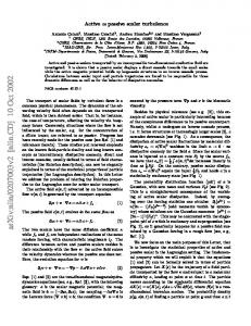
Typical spectra for both the velocity and scalar fluctuation fields with the passive grids 共R␭ = 66, R␭ = 170兲 and active grid 共R␭ = 500兲 are shown in Fig. 1. As has been previously observed,2,27,28 the scalar spectrum has a larger scaling range than the velocity field at the same R␭ (and at very low R␭ a scaling range exists for the scalar in the absence of a scaling region for the velocity27–29). This is presumably due to the existence of the ramp-cliff structures. Figure 2 shows longitudinal and transverse temperature SFs, 具⌬␪共x兲n典 / 共␪rms兲n and 具⌬␪共y兲n典 / 共␪rms兲n, respectively, for both passive and active grid experiments. 具⌬␪共x兲n典 is determined from Taylor’s hypothesis 共␦x = −U␦t兲 and thus the resolution is limited only by the sampling rate. On the other hand 具⌬␪共y兲n典 is determined by moving a temperature probe with respect to a fixed probe in the y direction and taking differences. Typically 15 points are taken and the resolution is not nearly as good as for the longitudinal direction. Nevertheless it is evident from Fig. 2 that 具⌬␪共y兲n典 / 共␪rms兲n and 具⌬␪共x兲n典 / 共␪rms兲n have approximately the same scaling exponents and their magnitudes appear to be the same. (Note that in Fig. 2 we have normalized the SFs by the local temperature rms values in order to compare the longitudinal and transverse SF scaling exponents. The normalizing variances are listed in the caption.) To more carefully check the relative


4014


FIG. 1. 1D velocity spectra (a) and scalar spectra (b) for the active grid and the passive grids. (a) Velocity spectra, u spectrum, solid line, v spectrum, dashed line. Upper curves, active grid 共R␭ = 480兲; middle curves, passive grid (M = 10.16 cm; LG, R␭ = 167); lower curves, passive grid (M = 2.54 cm; SG, R␭ = 66). The LG and the SG spectra have been divided by 100; (b) temperature spectra for the active grid, solid line; the LG, dashed line; the SG, long-dashed line. The Kolmogorov scale ␩ is defined in Table I, and k is the wavenumber (⬅2␲ f / U, where f is the spectral frequency and U is the mean velocity). In both (a) and (b) the straight line has a slope of −5 / 3.

slopes of the structure functions we examined their ratio for the active grid (not shown) and found that within the scaling range 共70⬍ r / ␩ ⬍ 400兲 it was ⬇1.1. The constancy of this ratio confirms that the scaling exponents of the longitudinal and transverse SFs are essentially the same in the inertialconvective subrange. (The transverse measurements for y / ␩ 艋 10 are prone to error because of the difficulty of determining y over small separations with the variable differencing probe, thus we do not report dissipation range measurements. Those measurements must be made with a fixed differential probe.17) We note the significant extension of the scaling range for the higher R␭ active grid case [contrast Fig. 2(b) with Fig. 2(a)]. We also note that the (anomalous) odd order transverse structure functions indicate a smaller integral scale than the corresponding even orders [this is particularly evident in Fig. 2(a)]. In Fig. 3 the third order longitudinal temperature structure functions, for both the active grid and the LG, are compared with their adjacent (second and fourth) order SFs.

A. Gylfason and Z. Warhaft

FIG. 2. Longitudinal (lines) and transverse (symbols) normalized structure functions, 共具⌬␪n典 / 共␪rms兲n兲, as a function of r / ␩. The magnitudes of the structure functions have been rescaled for clarity. (a) LG, R␭ = 154, (b) active grid, R␭ = 500. For both (a) and (b): 0.01具⌬␪2典 / 共␪rms兲2, solid line and open circles; 0.1具⌬␪3典 / 共␪rms兲3, filled circles; 0.1具⌬␪4典 / 共␪rms兲4, short-long dashed line and open squares; 具⌬␪5典 / 共␪rms兲5, filled squares; 具⌬␪6典 / 共␪rms兲6, long dashed line and open diamonds; 10具⌬␪7典 / 共␪rms兲7, filled diamonds; 10具⌬␪8典 / 共␪rms兲8, short dashed line and crosses; 100具⌬␪9典 / 共␪rms兲9, filled triangles; 100具⌬␪10典 / 共␪rms兲10, dotted line and plus signs. In (a) ␪rms = 0.244 ° C for the transverse structure functions and ␪rms = 0.211 ° C for the longitudinal structure functions: they were measured on different days and thus have slightly different root mean square values. In (b) ␪rms = 0.708 ° C; the longitudinal and the transverse structure functions were measured in the same run.

Symmetry requires that all odd order longitudinal structure functions be zero, and we observe noisy third order SFs with absolute magnitudes generally two or more decades below the even orders. Note that even for the active grid, where there is a weak mean longitudinal temperature variation, the third order SF is negligible. Higher order longitudinal odd SFs (not shown) were also negligible. We now turn to the delicate issue of determining the scaling exponents ␨n of the structure functions in the inertialconvective range. Only even order longitudinal structure functions are considered since odd orders are negligible (Fig. 3). While Fig. 2 suggests there are clear scaling ranges, a more stringent test for their existence is to take the derivative of the structure function. This is done in Fig. 4 for n = 4, 8 for the active grid and the passive grids. In the active grid case, in the region 70⬍ x / ␩ ⬍ 400, the derivative is horizontal to



FIG. 3. Normalized longitudinal structure functions 共具⌬␪n典 / 共␪rms兲n兲 as a function of x / ␩, using same data as in Fig. 2. (a) LG, (b) active grid. 具⌬␪2典 / 共␪rms兲2, circles; 兩具⌬␪3典 / 共␪rms兲3兩, diamonds; 具⌬␪4典 / 共␪rms兲4, squares.

within ±5% defining the extent of the scaling range. The passive grids have much narrower scaling ranges and for the small grid, a reliable scaling of the structure function is not possible. While a scaling range is present at least for the active grid and to a lesser degree for the LG, a further issue that must be addressed is the effect of the tunnel walls on the value of ␨n. The determination of higher order exponents is dependent on resolving large, rare temperature fluctuations. In a wind tunnel with a mean scalar gradient the temperature is bounded by the hot and cold walls and there is a clear possibility of truncation effects. In order to check for these effects we examined the probability density functions (pdf) of the temperature signals, the longitudinal scalar derivatives and scalar differences within the inertial-convective subrange, Fig. 5. Figure 5(a) shows pdfs of the temperature signals for the three grids. The SG has approximately exponential tails for the temperature pdf, a result obtained in previous

FIG. 4. Differentiated longitudinal structure functions for the SG (bottom curves), the LG (shifted up by 1, middle curves), and the active grid (shifted up by 2, top curves), ⳵ ln具⌬␪n典 / ⳵ ln共x兲. n = 4, solid line. n = 8, dashed line. The vertical bars indicate the extent of the inertial-convective subrange for each grid.


4015

experiments,14,30 and suggested by phenomenological models.31 Here the turbulence integral scale is sufficiently small, relative to the tunnel width, for rare, anomalous fluctuations to arrive at the measuring position from large, upstream transverse separations.2,31 The LG also shows evidence of exponential tails but with a narrower distribution. Here the wall effects are beginning to become significant. Finally for the active grid case the wall effects are much more severe because of the large integral scale. The temperature pdf now becomes sub-Gaussian since the large fluctuations are clipped by the maximum and minimum temperatures at the tunnel walls. This behavior is also observed in numerical work32 and other experiments.15,33 Table I lists the integral length scales and other relevant parameters for each of the three flows. The truncation effect does not prohibit us from looking at scaling exponents of the temperature structure functions but rather limits the order to which they can be resolved. Figure 5(b) shows the difference pdf is relatively unaffected until approximately when it crosses the temperature pdf, where it becomes truncated. This is particularly evident for the right-hand side of the difference pdf. (It can be shown analytically34 that the difference pdfs are bounded by the signal.) The wall effects manifest themselves in the difference pdfs of both the large passive grid and the active grid, causing them to become concave, at ⬇5⌬␪ / ⌬␪rms, Figs. 5(c) and 5(d), but for the SG, with its small integral scale, the difference pdfs remain exponential. It is therefore tempting to conclude that in absence of wall effects the pdfs of both the temperature and the temperature difference have approximately exponential tails. Figure 6 shows convergence plots 共⌬␪兲npdf共⌬␪兲 for n = 8, 10. The pdfs are well converged to tenth order. From Fig. 6 we conclude that the truncation of the pdfs at ⌬␪ / ⌬␪rms = 5 limits our scaling exponent range, at least for the active grid, to ␨10. For the passive grids, 5⌬␪rms is equivalent to about 0.3 ° C temperature difference for the small grid and 1 ° C for the large grid. In both cases the maximum temperature difference, set by the wall temperatures, is about 4.5 ° C. For the active grid 5⌬␪rms amounts to 2 ° C temperature difference while the difference between the wall temperatures is about 2.5° C. Thus for this case 5⌬␪rms is nearly equal to the limit set by the hot and the cold extremes of the tunnel. Figure 7 shows the compensated longitudinal structure functions for n = 2 – 10 for the active grid. The compensation was done both by eye and by using the extended self similarity (ESS) procedure,35 and these methods were found to agree well. In order to test the subjective variation caused by the visual fitting we varied the compensation. Figure 7 shows the sixth order structure function compensated with exponents 1.105 and 1.125. Even for a variation of less than 1% there is a marked difference in the plateau. For smaller variations it was difficult to detect any difference in the plateau and we will use ±0.01 as the error in determining ␨6 (it is slightly greater for the higher orders). Other sources of error including the convergence of the probability density functions are discussed below. Figure 8 shows ␨n as a function of n for both the LG [Fig. 8(a)] and for the active grid [Fig. 8(b)]. From here on


4016



FIG. 5. The pdfs of the temperature signals, the temperature derivatives and the temperature differences over longitudinal separations. (a) pdf of the temperature signal vs ␪ / ␪rms. SG, open circles; LG, squares; active grid, filled circles. The lines are Gaussian curve fits to each pdf. (b) pdf of the temperature signal (filled circles) and temperature difference for inertial-convective range separation r / ␩ = 200 (open circles) for the active grid. Arguments are normalized by ␪rms. (c) pdf of temperature derivatives and differences for the passive grids. SG (upper curves). All of these curves are multiplied by 1000 for clarity. pdf关⳵␪ / ⳵x / 共⳵␪ / ⳵x兲rms兴, open circles; r = 40␩, filled circles; r = 60␩, open squares; r = 200␩, filled squares. The LG (lower curves). pdf关⳵␪ / ⳵x / 共⳵␪ / ⳵x兲rms兴, open circles; r = 44␩, filled circles; r = 72␩, open squares; r = 116␩, filled squares; r = 218␩, diamonds. (d) pdf of derivatives and differences for the active grid. pdf关⳵␪ / ⳵x / 共⳵␪ / ⳵x兲rms兴, open circles; r = 50␩, filled circles; r = 100␩, open squares; r = 250␩, filled squares; r = 400␩, diamonds; r = 800␩, crosses. The vertical lines are the location of the peak of the tenth moment of the pdfs at r = 72␩ in (c), and r = 250␩ in (d), see Fig. 6.

we disregard the SG results because of their small inertialconvective subrange (Fig. 4). Experiments were conducted on different days and the variation in ␨n tends to reflect scatter rather than a dependence on R␭, although there does appear to be a systematic variation for the active grid where ␨2 increases from 0.64 to 0.68 with increasing R␭ [Fig. 8(b)]. This was not fully supported by some other of our experiments and may be due to the x / M variation, which was not systematically explored. For the passive grid the variation in ␨2 was from 0.65 to 0.67 but scattered as a function of Reynolds number 共150艋 R␭ 艋 167兲. Thus over the full Reynolds number range 共150艋 R␭ 艋 700兲 we see no systematic variation. Notice that there is not much evidence that the scaling exponent is saturating. We will return to this in Sec. IV. At second order the SF scaling exponent varied from 0.64 to 0.68, as compared to the KOC scaling of 2 / 3. We

ascribe this variation to scatter, since we were unable to find any systematic cause for it. Other studies also show variation in ␨2 (Table II). In order to facilitate comparisons of our various experiments, and comparisons with that of other workers (below), we have normalized the data of Figs. 8(a) and 8(b) with ␨2. These results are shown in Fig. 9. The collapse is good. No systematic Reynolds number effect is observed. We have fitted a logaritmic curve to our data: the best fit is ␨n / ␨2 = 0.507+ 1.633 ln n 共2 艋 n 艋 10兲. Hence ␨n is still increasing at n = 10, albeit at a slower rate. Our results do not preclude saturation at higher order, although it would be rash to infer it from the present data. Clearly, if saturation does occur it does so for n ⬎ 10 at least for this flow.36 Note that there is no significant difference between the scaling exponents for the active grid and the large passive grid, providing further evidence that the truncation effects are not




4017

FIG. 6. nth moment of pdfs of temperature differences over inertialconvective range separation 共⌬␪兲npdf共⌬␪兲 vs ⌬␪ / ⌬␪rms. The curves are normalized such that the area is unity. LG, n = 8, circles; n = 10 (shifted up by 0.2), squares. Active grid, n = 8 (shifted up by 0.4), diamonds; n = 10 (shifted up by 0.6), crosses.

FIG. 8. The scaling exponents ␨n of the longitudinal temperature structure function vs order n. (a) The LG. R␭ = 150, circles; R␭ = 155, squares; R␭ = 158, diamonds; R␭ = 160, crosses; R␭ = 167, plus signs. (b) The active grid. R␭ = 480, filled circles; R␭ = 560, filled squares; R␭ = 688, filled triangles; the lines are logaritmic curve fits.

playing a significant role for the active grid (for which the integral scale is much larger). Figure 9 also shows the scaling exponent of the transverse structure functions. As previously mentioned the results are quite similar to that of the longitudinal structure functions but the error in estimating the exponents is much greater (see error bar on the graph). For this reason we have plotted this exponent only up to the eighth order.

⬃0.3; at tenth order it is ⬃0.5. The data of Meneveau et al.22 and Moisy et al.23 appear to be saturating, but the rate at which this occurs, and the magnitude of ␨⬁, is quite different for each data set. All other data show a decrease in the rate of change in ␨n, but saturation is not evident, at least to the 12th order. Differences in boundary conditions, wall effects, and poor convergence of the data are probable reasons for the variations between the data sets of Fig. 10. Table II lists the different types of flows investigated as well as the values of

IV. COMPARISON WITH OTHER EXPERIMENTS

Figure 10 shows a compilation of a number of other experiments previously reported in the literature. Also included are our results from Fig. 9. Large variation is evident, not only for the higher orders, but even at fourth and sixth orders. For example at the sixth order there is a variation of

TABLE II. The flows and values ␨2 for the various scalar experiments showns in Fig. 10. Author

Flow

␨2

Chen and Caoa

DNS 共5123兲 Isotropic turbulence

0.606± 0.019

Moisy et al.b

Cylindrical vessel with rotating disks

0.45–0.65, increases with R␭

Antonia et al.c Ruiz-Chavarria et al.d

Shear flows Shear flow (cylinder) with mandoline

0.63 0.62

Meneveau et al.e

Wake of heated cylinder Exponents calculated using joint multifractals

0.62

Mydlarski and Warhaftf

Decaying grid turbulence with transverse temperature gradient

0.66

Celani et al.g

2D Gaussian velocity field Decaying grid turbulence with transverse temperature gradient

0.65 0.65–0.68, no apparent R␭ dependence (see text)

Present work

a

FIG. 7. Compensated longitudinal structure functions vs x / ␩ for the active grid. x−0.640具⌬␪2典, open circles; x−0.940具⌬␪4典 / 4, squares; x−1.115具⌬␪6典 / 25, filled circles; x−1.248具⌬␪8典 / 220, crosses; x−1.349具⌬␪10典 / 2500, plus signs. Also shown in the sixth order longitudinal structure function compensated with different exponents to demonstrate error in determining the scaling exponents. x−1.105具⌬␪6典 / 25, diamonds; x−1.125具⌬␪6典 / 25, triangles.

Reference 25. Reference 23. c Reference 21. d Reference 24. e Reference 22. f Reference 2. g Reference 9. b


4018


FIG. 9. Normalized scaling exponents ␨n / ␨2 as a function of order n for all the data of Figs. 8(a) and 8(b) using the same symbols. The plus signs are the normalized scaling exponents for the transverse structure functions. The error bar is given at the seventh order. The solid line is a logaritmic curve fit to the longitudinal structure function, ␨n / ␨2 = 0.507+ 1.633 ln共n兲.

␨2. As in the present work, there is large variation in ␨2 and this variation is systematically amplified at higher orders. This is particularly evident in our own experiments (Fig. 8). While we do not have any compelling evidence to reject the data of other workers, a reanalysis of Mydlarski and Warhaft15 (see Fig. 11 of Warhaft2) has indicated that the data suffer from convergence problems for n 艌 8. It is also relevant to note that the data of Meneveau et al.22 were obtained from analysis of experimental data by using joint multifractal formalism while for all the other data the scaling exponents were determined either directly from the structure function or by using ESS. Note the large difference between


the two numerical simulation experiments, those of Chen and Cao,25 and Celani et al.9 The most recent other laboratory experiment is by Moisy et al.23 Their fluid is low temperature helium gas in a closed cylinder, with rotating disks stirring the fluid. A small heated grid (mandoline) is positioned at the edge of the cylinder and the cold wire anemometer is positioned 20 mesh lengths downstream from it. Both the velocity and thermal fields are undoubtedly complex. Nevertheless these workers show pdfs that are well converged. Notice that the difference between the Moisy et al.23 experiment and the present work is most pronounced at the sixth order where the statistics are well converged and finite domain effects are even less significant than at higher orders. The difference between their data and that of the present work is then presumably due to the difference in boundary conditions. In Moisy et al.23 the temperature length scale is determined by both the velocity field and the mesh of the heated grid, whereas in our work the thermal scale is determined purely by the velocity field. Further, in the present work there is a mean scalar gradient as opposed to the mandoline generated fluctuating thermal field in the Moisy et al.23 experiment. V. CONCLUSIONS

A compilation of the present work with that of previous experiments shows that the way the scalar structure function exponent ␨n varies with order n is far from resolved. The present work shows that ␨n is still increasing at n = 10, but saturation cannot be ruled out at high orders. Our results, for a passive cross-stream gradient in decaying grid turbulence, are independent of Reynolds number 共150艋 R␭ 艋 700兲 and ␨n is almost the same for the transverse and longitudinal structure functions (Fig. 9), indicating that the ramp-cliff struc-

FIG. 10. Normalized scaling exponents ␨n / ␨2 as a function of order n. Open circles, Meneveau et al. (Ref. 22); open squares, Antonia et al. (Ref. 21); diamonds, Celani et al. (Ref. 9); crosses, Chen and Cao (Ref. 25); plus signs, Moisy et al. (Ref. 23); triangles, Warhaft (Ref. 2); solid circles, RuizChavarria et al. (Ref. 24). The solid thick line is the curve fit to all of our data (Fig. 9). [It is extrapolated to n = 12 in order to compare with the experiment of Moisy et al. (Ref. 23) and shown as the short dashed line.] The thick dashed line is a curve fit to the Moisy et al. (Ref. 23) data: ␨n / ␨2 = A共1 − e−bx兲. Thin solid lines are smoothed curves through each data set. The long dashed line is the KOC scaling.



tures are ubiquitous, despite their preferential alignment along the mean gradient. Our results show negligible odd order structure functions in the longitudinal direction (consistent with symmetry requirements, Fig. 3) but for the transverse direction their exponents evolve monotonically with those of the even exponents, a result consistent with previous findings.2 The existence of the odd order transverse structure functions is due to the anisotropic ramp-cliff structures. Our experiments also show the effect of finite temperature extremes set by the flow domain. The scalar signal pdf has exponential tails when wall effects are negligible and subGaussian tails when they are significant [Fig. 5(a)]. Previous results (Fig. 10) show saturation of ␨n for some experiments but not for others. Reasons for the variations are attributed to statistical convergence problems (at high orders), problems due to finite domain size causing clipping of large rare fluctuations (both in experiments and computations), and differences in boundary conditions. The latter appears to be dominant when the present work, with the crossstream scalar gradient, is compared to the decaying (mandoline generated) temperature fluctuations of the Moisy et al.23 experiment where there is no mean temperature gradient. The Moisy et al.23 experiment shows saturation, and even at the sixth order (where statistical and finite domain effects can be ruled out) there is a significant difference between ␨n in the two experiments. These results suggest that boundary conditions are affecting the values of ␨n. Whether it is differences in the velocity field, or in the scalar field itself, that causes the differences in the scaling exponents, needs to be resolved. Clearly, more experiments are suggested. In particular, it would be interesting to repeat the experiments reported here, but in a facility with sufficient dimensions so that wall effects are eliminated completely. ACKNOWLEDGMENTS

The authors thank Laurent Mydlarski, Ed Jordan, and Sathyanarayana Ayyalasomayajula for their help. This work was supported by the U.S. National Science Foundation. 1

B. I. Shraiman and E. D. Siggia, “Scalar turbulence,” Nature (London) 405, 639 (2000). 2 Z. Warhaft, “Passive scalars in turbulent flows,” Annu. Rev. Fluid Mech. 32, 203 (2000). 3 R. H. Kraichnan, “Small-scale structure of a scalar field convected by turbulence,” Phys. Fluids 11, 945 (1968). 4 R. H. Kraichnan, “Passive scalar convection by a quasi-uniform random straining field,” J. Fluid Mech. 64, 737 (1974). 5 R. H. Kraichnan, “Anomalous scaling of a randomly advected passive scalar,” Phys. Rev. Lett. 72, 1016 (1994). 6 M. Chertkov, G. Falkovich, I. Kolokolov, and V. Lebedev, “Normal and anomalous scaling of the 4th order correlation function of randomly advected passive scalar,” Phys. Rev. E 52, 4924 (1995). 7 K. Gawedzki and A. Kupiainen, “Anomalous scaling of the passive scalar,” Phys. Rev. Lett. 75, 3834 (1995). 8 B. I. Shraiman and E. D. Siggia, “Anomalous scaling of a passive scalar in a turbulent flow,” C. R. Acad. Sci. III 321, 279 (1995). 9 A. Celani, A. Lanotte, A. Mazzino, and M. Vergassola, “Universality and saturation of intermittency in passive scalar turbulence,” Phys. Rev. Lett. 84, 2385 (2000). 10 M. Holzer and E. D. Siggia, “Turbulent mixing of a passive scalar,” Phys.


4019

Fluids 6, 1820 (1994). A. Pumir, “A numerical study of the mixing of a passive scalar in 3 dimensions in the presence of a mean gradient,” Phys. Fluids 6, 2118 (1994). 12 G. Falkovich, K. Gawedzki, and M. Vergassola, “Particles and fields in fluid turbulence,” Rev. Mod. Phys. 73, 913 (2001). 13 R. Budwig, S. Tavoularis, and S. Corrsin, “Temperature fluctuations and heat flux in grid generated isotropic turbulence with streamwise and transverse mean-temperature gradients,” J. Fluid Mech. 153, 441 (1985). 14 Jayesh and Z. Warhaft, “Probability distribution, conditional dissipation, and transport of passive temperature fluctuations in grid generated turbulence,” Phys. Fluids A 4, 2292 (1992). 15 L. Mydlarski and Z. Warhaft, “Passive scalar statistics in high-Pécletnumber grid turbulence,” J. Fluid Mech. 358, 135 (1998). 16 A. Sirivat and Z. Warhaft, “The effect of a passive cross-stream temperature gradient on the evolution of temperature variance and heat flux in grid turbulence,” J. Fluid Mech. 128, 326 (1983). 17 C. Tong and Z. Warhaft, “On passive scalar derivative statistics in grid turbulence,” Phys. Fluids 6, 2165 (1994). 18 S. Chen and R. H. Kraichnan, “Simulations of a randomly advected passive scalar field,” Phys. Fluids 10, 2867 (1998). 19 L. Mydlarski and Z. Warhaft, “Three-point statistics and the anisotropy of a turbulent passive scalar,” Phys. Fluids 10, 2885 (1998). 20 L. Mydlarski, A. Pumir, B. I. Shraiman, E. D. Siggia, and Z. Warhaft, “Structures and multipoint correlators for turbulent advection: Predictions and experiments,” Phys. Rev. Lett. 81, 4373 (1998). 21 R. A. Antonia, E. J. Hopfinger, Y. Gagne, and F. Anselmet, “Temperature structure functions in turbulent shear flows,” Phys. Rev. A 30, 2704 (1984). 22 C. Meneveau, K. R. Sreenivasan, P. Kailasnath, and M. S. Fan, “Joint multifractal measures: Theory and applications to turbulence,” Phys. Rev. A 41, 894 (1990). 23 F. Moisy, H. Willaime, J. S. Andersen, and P. Tabeling, “Passive scalar intermittency in low temperature helium flows,” Phys. Rev. Lett. 86, 4827 (2001). 24 G. Ruiz-Chavarria, C. Baudet, and S. Ciliberto, “Scaling laws and dissipation scale of a passive scalar in fully developed turbulence,” Physica D 99, 369 (1996). 25 S. Chen and N. Cao, “Anomalous scaling and structure instability in threedimensional passive scalar turbulence,” Phys. Rev. Lett. 78, 3459 (1997). 26 K. Yoon and Z. Warhaft, “The evolution of grid-generated turbulence under conditions of stable thermal stratification,” J. Fluid Mech. 215, 601 (1990). 27 Jayesh, C. Tong, and Z. Warhaft, “On temperature spectra in grid turbulence,” Phys. Fluids 6, 306 (1994). 28 T. T. Yeh and C. W. van Atta, “Spectral transfer of scalar velocity fields in heated-grid turbulence,” J. Fluid Mech. 58, 233 (1973). 29 Z. Warhaft and J. L. Lumley, “An experimental study of the decay of temperature fluctuations in grid-generated turbulence,” J. Fluid Mech. 88, 659 (1978). 30 B. R. Lane, O. N. Mesquita, S. R. Meyers, and J. P. Gollub, “Probability distributions and thermal transport in a turbulent grid flow,” Phys. Fluids A 5, 2255 (1993). 31 A. Pumir, B. Shraiman, and E. D. Siggia, “Exponential tails and random advection,” Phys. Rev. Lett. 66, 2984 (1991). 32 A. Celani, A. Lanotte, A. Mazzino, and M. Vergassola, “Fronts in passive scalar turbulence,” Phys. Fluids 13, 1768 (2001). 33 M. Ferchichi and S. Tavoularis, “Scalar probability density function and fine structure in uniformly sheared turbulence,” J. Fluid Mech. 461, 155 (2002). 34 A. Noullez, G. Wallace, W. Lempert, R. B. Miles, and U. Frish, “Transverse velocity increments in turbulent flow using the relief technique,” J. Fluid Mech. 339, 287 (1997). 35 R. Benzi, S. Ciliberto, R. Tripiccione, C. Baudet, F. Massaioli, and S. Succi, “Extended self similarity in turbulent flows,” Phys. Rev. E 48, R29 (1993). 36 If the difference pdfs have pure exponential tails then it can be shown that ␨n increases linearly with n at high orders. More work is required to determine the effects of varying the scalar signal pdf on the scalar structure function exponents. 11
