moving eastward along the continental shelf break line. (Figure 3a). ... break line in a cyclonic direction; (b) 1982 â AW flow declines to the ..... overview.html).
JOURNAL OF GEOPHYSICAL RESEARCH, VOL. 112, C04S05, doi:10.1029/2006JC003734, 2007
On improving the simulation of Atlantic Water circulation in the Arctic Ocean E. N. Golubeva1 and G. A. Platov1 Received 30 May 2006; revised 27 December 2006; accepted 24 January 2007; published 11 April 2007.
[1] We performed a set of numerical experiments in order to better simulate the
circulation of Atlantic Water in the Arctic Ocean by employing a coupled ice-ocean Arctic regional model. We found that the inflow of Atlantic Water via Fram Strait is weak in the case of high viscosity and diffusivity coefficients (1 � 108 cm2/s and 1 � 107 cm2/s) and creates an anticyclonic circulation in the Eurasian basin. This flow increases significantly when both coefficients are scaled down (to 1 � 107 cm2/s and 0.5 � 106 cm2/s) but the current path is then unstable, and it becomes mostly anticyclonic after about a decade of integration. A further reduction of these coefficients leads to growing instabilities due to insufficient grid resolution. Short-term integration of the model with doubled space resolution shows better agreement with observations, but long-term calculation is still restricted by simulation time. Alternatively, a lower resolution version of this model benefits from parameterizations of subscale processes. Incorporation of the Neptune parameterization of eddy-topography interaction into the model intensifies the current steered by subsurface topography and results in cyclonic circulation of the Atlantic Water in every subbasin and in the whole Arctic region. In the absence of salinity restoring there was strong salinity drift at the surface, resulting in a salinity increase in the central Arctic by 3 units from 1960 to 2005. The Arctic freshwater content is driven basically by year-to-year variations of convective mixing involving more saline water from lower layers. After cooling and increasing in salinity through brine rejection, the surface water becomes denser, leading to even stronger convective mixing. One-dimensional model tests showed how model performance could be improved by implementing a lower vertical diffusion coefficient and higher vertical resolution. Citation: Golubeva, E. N., and G. A. Platov (2007), On improving the simulation of Atlantic Water circulation in the Arctic Ocean, J. Geophys. Res., 112, C04S05, doi:10.1029/2006JC003734.
1. Introduction [2] The Arctic Ocean has received considerable attention during the last several decades because of remarkable changes revealed by observations in the Arctic atmosphere-ice-ocean system. Comparison of observed temperature from the 1990s with the previous period (1955 – 1989) shows stable temperature rise in the water supplied by the Atlantic Ocean [e.g., Quadfasel et al., 1991; Carmack et al., 1995; Swift et al., 1997]. This temperature anomaly, along with some other changes in the atmosphere and the sea ice, stimulated a number of research projects devoted to a comprehensive Arctic investigation. So far, it is not clear whether this temperature rise is a result of global warming caused by human activity or a manifestation natural oscillations in the Arctic climate system. [3] Atlantic Water (AW) has long been a focus of thorough investigations of the Arctic Ocean. As early as 1 Institute of Computational Mathematics and Mathematical Geophysics, Siberian Branch of the Russian Academy of Sciences, Novosibirsk, Russia.
Copyright 2007 by the American Geophysical Union. 0148-0227/07/2006JC003734
1902, Nansen developed the basic hypothesis for AW transport into the Arctic Ocean and its further circulation in the Arctic basin. During the last century, this point was widely discussed and developed by many authors, including Timofeev [1960], Coachman [1969], Lewis [1982], and Aagaard [1982]. Timofeev [1960] deduced one of the first patterns of AW circulation based on its thermal properties. According to this pattern, the AW creates a giant cyclonic gyre centered between the North Pole and the Fram Strait. Over a number of years, this pattern was refined by Coachman [1969], Treshnikov and Baranov [1972], and Nikiforov and Shpaikher [1980]. [4] Two branches of AW flow into the Arctic from the Norwegian Sea (Figure 1 shows a map of the region). The eastern branch of AW passes through the Barents Sea. Originally warm, it loses its heat because of intensive airsea exchange in the relatively shallow Barents Sea. Another branch, the West Spitsbergen Current, penetrates to the Arctic Ocean via Fram Strait, mixes with cold and fresh Arctic surface water, sinks to the intermediate depth level, and flows farther into the Arctic Ocean along the continental slope. AW is a major potential source of heat for the entire Arctic Ocean [Aagaard and Greisman, 1975]. These
C04S05
1 of 16
C04S05
GOLUBEVA AND PLATOV: ON IMPROVING THE SIMULATION OF AW
C04S05
Figure 1. A map of the Arctic region with the geographic names used in the text. branches of AW join in the vicinity of St. Anna Trough and move eastward along the continental slope. The observationbased AW circulation scheme proposed by Rudels et al. [1994] shows the cyclonic gyres within the Nansen, Amundsen, and Canadian basins of the Arctic Ocean. [5] Along with interpretation of the observational water temperature and salinity data, numerical modeling is a useful tool to better understand 3-D water motion. The numerical AW investigations reported in the literature are aimed at obtaining knowledge of AW dynamics and to understanding the climatic changes of AW during recent decades. For proper numerical investigation of AW dynamics, reproduction of cyclonic AW flow is a key factor. However, AW circulation patterns differ significantly from model to model [Hakkinen and Mellor, 1992; Holland et al., 1996; Nazarenko et al., 1998; Zhang et al., 1998a; Yakovlev, 1998; Karcher and Oberhuber, 2002; Karcher et al., 2003; Steiner et al., 2004]. Among these models, for example, some reproduce cyclonic circulation of AW, but others show flow in the opposite direction [Proshutinsky et al., 2005]. [6] Employing a coupled ice-ocean model, this paper presents results of a set of numerical experiments in order to provide a better description of AW cyclonic circulation in the Arctic. These experiments include model runs (1) with different coefficients of horizontal diffusivity and viscosity
(Experiment 1); (2) with different model resolutions (Experiment 2); and (3) with a parameterization of eddytopography interaction known as the Neptune effect proposed by Holloway [1987] (Experiment 3). These experiments were carried out with water temperature and salinity restoring at the sea surface. The temperature and salinity fields were interpolated onto the model grid from the Levitus and Boyer [1994] and Levitus et al. [1994] climatologies and the restoring period was 30 days. Experiment 4 was designed to follow the Arctic Ocean Model Intercomparison Project (AOMIP) coordinated model run conditions. In this experiment no restoring was applied after 1960. As compared to the previous experiments, the restoring shut-off has a significant impact on Arctic Ocean stratification. Possible directions for model improvement are discussed in the final section.
2. Model and Data [7] The World Ocean Circulation Model designed at the Institute of Computational Mathematics and Mathematical Geophysics (ICMMG model) [Kuzin, 1985; Golubeva et al., 1992] has been adopted for the Arctic Ocean domain. The model was formulated with hydrostatic, Boussinesq, and rigid-lid approximations. There are no heat and salt fluxes
2 of 16
GOLUBEVA AND PLATOV: ON IMPROVING THE SIMULATION OF AW
C04S05
Figure 2. The model domain in the area of the Canadian straits. The bold dots represent model grid nodes. Bold solid contours are the model boundaries. Light solid contours are the geographic coastline. Some nodes were added by hand to make straits at least 2 nodes wide.
via bottom and solid model domain boundaries. A no-slip condition for velocity and a quadratic drag bottom friction with a coefficient of 2 � 10�3 are applied. [8] The discretization of the ICMMG model equations is conducted using curvilinear orthogonal coordinates and the finite element method, along with a splitting technique applied for coordinates and physical processes. The model dynamics are resolved by separating barotropic and baroclinic modes. The barotropic mode is described in terms of a stream function. The model time-step is two hours. More details about the numerical model can be found in Appendix A. [9] The sea ice model is an elastic viscous-plastic model, which is a modification of the viscous-plastic model by Hibler [1979]. The set of model parameters is given by Holloway et al. [2007]. [10] The list of forcing data for the sea ice model includes wind speed, surface-ocean velocities, specific humidity, air density and temperature, incoming shortwave and longwave radiation, evaporation and precipitation rates, sea-surface temperature and salinity, and sea-surface tilt. The characteristics provided by the sea ice model for the ocean include the value of penetrating shortwave radiation; fluxes of heat, salt, and fresh water; and the ice-water stress. [11] The initial ice distribution was prescribed as ice 2 m thick with compactness of 0.9 in the areas of negative air
C04S05
temperature. A seven-year spin-up run provides more reasonable sea ice distribution, which is further used as the initial sea ice state. [12] The characteristics of the lower atmosphere and radiation are prescribed, taken from NCEP/NCAR reanalysis [Kalnay et al., 1996]. The wind forcing is a combination of data from Trenberth et al. [1989] for lower latitudes ( 0 in the Fram Strait. Arctic Ocean. There were warm periods during the mid to late 1950s, from 1963 to 1969, and in the early 1990s, and a cold period prevailed from 1974 to the end of the 1980s. The warm period of the early 1990s identified in their study
C04S05
is consistent with the anomaly in the Fram Strait and propagation of the anomaly along the shelf break by the boundary current. With respect to the 1960s, Swift et al. [2005] found that the warming had a nonadvective origin, so it did not begin in Fram Strait. They suggest diapycnal heat loss from the warm Atlantic core. The coldest anomalies during the 1970s and 1980s in the data analysis have reasonable consistency with enhanced cooling of shelf waters entering the Arctic Ocean via the Laptev Sea or, possibly, the Kara Sea. [34] Model sensitivities to wind stress variations were analyzed in Experiment 3. Both observations and model results by Anderson et al. [1994], Quadfasel et al. [1991], Steele and Boyd [1998], Grotefendt et al. [1998], Polyakov et al. [2004], Zhang et al. [1998b], Karcher et al. [2003], and Gerdes et al. [2003] show that propagation of a warm AW signal in the intermediate Arctic layer in the 1990s occurred under the high NAO state that resulted in intensified transport in the West Spitsbergen Current and the Barents Sea outflow. Figure 9 shows annual simulated mass and heat transport of AW through Fram Strait for ICMMG Experiment 3. The general tendency is toward increasing water and heat transport for the entire modeling period, with maximum values in the early 1990s. Figure 10 shows how the simulated warm signal spreads with the main boundary
Figure 10. Warming of the Atlantic layer in Experiment 3. Temperature distribution at 200 m depth (a) in 1990, (b) in 1992, (c) in 1994, and (d) in 1996. 8 of 16
C04S05
GOLUBEVA AND PLATOV: ON IMPROVING THE SIMULATION OF AW
C04S05
Figure 11. Warming of the Atlantic layer. Temperature section (marked in Figure 4) in Experiment 3: (a) distribution in 1989 and (b) distribution in 1996. current from 1990 to 1996. Warm water from Fram Strait is transported by the boundary current along the continental slope and reaches Franz Josef Land. In the region of St. Anna Trough, this signal diminishes. We speculate that this happens because of the Barents Sea branch contribution, which is cooler than the Fram Strait branch due to heat loss in the shallow Barents Sea. The lower signal spreads farther to the Lomonosov Ridge, and then splits into two branches, following the circulation pattern. Vertical sections of the temperature field (Figure 11) show that the temperature in the core of the AW rose by 0.5 degrees from 1989 to 1996. This model result for the 1990s Arctic warming event is consistent with the observational data and model studies cited above. 3.4. Experiment 4 [35] This experiment was designed to satisfy conditions of the AOMIP coordinated model run (http://fish.cims. nyu.edu/project_aomip/experiments/coordinated_analysis/overview.html). According to this protocol, the surface restoring of salinity is stopped after the first eleven years (1948 – 1958). Some results from this ICMMG model output are also presented by Holloway et al. [2007]. [36] In the absence of salinity restoring, the model surface salinity tends toward values higher than those observed in the Arctic Ocean. In the real Arctic Ocean, fresh water covers the top of the water column. Even in cases of very strong cooling, the low salinity prevents the surface water from becoming more dense than the lower water column, at least in the central Arctic. Thus, the upper ocean stratification is very strong and stable. In experiment 4, however, a strong drift of the surface salinity occurred, resulting in an increase in salinity in the center of the basin by 3 units from 1960 to 2005 (Figure 12).
[37] It should be noted here that such an increase in upper layer salinity does not violate salt conservation by the model. The freshwater content could be presented in terms of a salinity deficit integrated over the whole Arctic.
Figure 12. Increasing the surface salinity in a coordinated AOMIP run (Experiment 4) without restoring to surface salinity. Salinity distribution: (a) in 1960 and (b) in 2000.
9 of 16
C04S05
GOLUBEVA AND PLATOV: ON IMPROVING THE SIMULATION OF AW
Figure 13. The time series related to the freshwater volume:R (a) freshwater content in terms of the salinity deficit (34.8 � S) dV integrated over the volume, where (34.8 � S) > 0, (b) saline water transport (positive is northward) with S > 34.8 psu at 70°N in the North Atlantic, and (c) freshwater transport (negative is southward) with S < 34.8 psu at 70°N. R Figure 13a presents a time series of the value (34.8 � S) dV, integrated over the volume, where S < 34.8 psu. It shows that freshwater content (or salinity deficit) increases from 1970 to 1984 (label B in Figure 13), then exibits a small minimum in 1988 (label C) and another maximum in 1993 (label D). Starting in 1993 the freshwater content steadily decreases. In contrast, both the inflow transport of saline Atlantic water with S > 34.8 (Figure 13b) and the freshwater content (Figure 13a) show maxima and minima at the same time. This means that freshwater content is not caused by Atlantic water inflow, i.e., the greater the value of the freshwater content, the more AW is contributed. The freshwater outflow transport (Figure 13c) reaches maxima (negative values correspond to southward transport) at the same time as freshwater content maxima. The exception is 1982 (label A) when the outflow maximum is two years earlier then the freshwater content maximum. Nevertheless, the freshwater outflow appears to be the consequence of Arctic freshwater content rather than its cause. In this case, what could be the main reason for Arctic freshwater content changes? All other factors, such as precipitation, river discharge, and Pacific water inflow, are steady, that is, one year is similar to any other. The likely reason could be that these waters are more or less mixed with others in different years, which may be caused by lateral diffusion and/or convective mixing. [38] In the late 1990s, there was strong convection accompanied by decreasing freshwater content, which confirms the idea presented in the previous paragraph.
C04S05
[39] At some stage after cooling and increased salinity due to ice formation, the surface water becomes dense enough to produce unstable stratification, leading to convective mixing. The boundary current travels in a cyclonic direction, stabilized by the Neptune parameterization. Due to the convective exchange, AW shares its heat with the top layers by making them warmer. This in turn affects the ice cover. Under these circumstances, new ice formation is hampered and existing ice melts more easily. As a consequence, the ice thickness and compactness decrease and the sea surface has wider areas free from ice. This enhances heat exchange with the atmosphere, making the top water layer colder in winter, which stimulates convection. The result of this progressive cooling and vertical mixing is presented in Figure 14. The mixed layer depth reaches 500 m at a temperature close to freezing. As for AW, it cools faster and cannot be traced far in the Arctic domain as identified by a temperature maximum. It is possible that the vertical resolution of the numerical model is not sufficient to support such a thin layer of relatively fresh water at the ocean surface without diffusive mixing with underlying water. Also, the parameterization for the vertical diffusion coefficient must assume a smaller value at the surface in the case of a strong ice cover, since the surface is not disturbed by wind waves as it is in ice – free ocean. Some 1-D tests were carried out to see how model performance could be improved by implementing a lower vertical diffusion coefficient and higher vertical resolution (see Appendix B). [40] In Experiment 1 and Experiment 3 no such breakdown of stratification was found due to the stabilizing effect of the restoring. Arctic modeling with and without climate restoring was investigated by Zhang et al. [1998a]. They found that the main deficiency of the Arctic model without restoring is its prediction of unrealistically high salinity in the central Arctic, which tends to weaken the ocean currents. The critical role of sea surface salinity restoring in the freshwater budget was discussed by Steele et al. [2001]. They reported that reduction in the strength of the restoring term leads to increasing salinity in the Beaufort Gyre. In Karcher et al. [2007], the existence of strong drift in model hydrography for the AOMIP models, when no restoring is used, prevents analysis of density layers in the coordinated AOMIP experiment after the first two decades. [41] Integral ice properties presented in Figure 15 show that ice volume (Figure 15b) grows during the 1970s and reaches its maximum value in 1978. This growth is accompanied by a subsequent increase in snow volume (Figure 15c) and ice-covered area (Figure 15d). Also, ice transport from the Arctic domain reaches 16 � 103 m3/s at the end of this period (Figure 15a). In the following 10 years, the total ice volume exhibits rather small variations, but it increases a bit in 1986 along with the snow volume and ice-covered area. Beginning in 1986 until the end of the run, the ice presence is slightly reduced, as is seen for all characteristics in Figure 15, but it is not because of outward ice transport, which also becomes smaller.
4. Conclusions [42] This paper analyzes and discusses a set of numerical experiments based on an ICMMG Atlantic-Arctic ice-ocean numerical model. The major goals of these experiments
10 of 16
C04S05
GOLUBEVA AND PLATOV: ON IMPROVING THE SIMULATION OF AW
C04S05
Figure 14. Cooling of the Atlantic layer in the coordinated AOMIP run (Experiment 4) without restoring to surface salinity. Temperature section (marked in Figure 7): (a) in 1960, (b) in 1992, and (c) in 2000. were to reproduce the basic features of AW in the Arctic Ocean and to recommend parameterizations appropriate for representing the AW cyclonic circulation pattern. [43] The viscosity terms are represented in the standard model code by Laplacian parameterizations. When the horizontal viscosity and diffusion coefficients have lower values (0.5 � 106 cm2/s for diffusivity and 1 � 107 cm2/s for viscosity), as compared to the standard values (1 � 107 cm2/s and 1 � 108 cm2/s, respectively), the flow of AW through Fram Strait into the Arctic Ocean becomes stronger. In this case, the flow extends farther east into the Arctic along the continental slope and forms an isobath –following current, which is in agreement with available observations. However, this current is not stable in time. Variations in the wind stress and wind – stress curl over the several decades of simulation cause the slope current to decline from the shelf break seaward and flow along the Lomonosov Ridge. The flow splits into two branches at the southernmost point of the Lomonosov Ridge. The first branch is more stable and continues to follow the cyclonic circulation, but the second one corresponds to the anticyclonic circulation pattern, which, according to ICMMG results, can change its trajectory again. Another branch of AW, which passes through the Barents Sea, becomes too weak to yield a reliable throughflow of AW via St. Anna Trough. [44] Following a study by Yang [2005], which found that the PV flux from sub-Arctic regions strongly controls the direction of AW circulation, PV fluxes across Fram Strait and St. Anna Trough were analyzed based on ICMMG model results. The analysis revealed that the Barents Sea was the dominant source of negative PV flux into the Arctic interior in the 1960s and 1970s. The Fram Strait contribution to the negative PV flux becomes more important beginning in the 1970s. The net PV flux for AW is negative in this experiment, and, according to Yang [2005], the anticyclonic circulation of AW should be established.
[45] Application of higher model resolution improves the pattern of the Barents Sea circulation, showing that intensive flow of modified AW through the St.\ Anna Trough appeared during the three-year model run. Also, the shelf
Figure 15. The time series related to the ice-snow cover: (a) the ice exported to the south at 70°N, the volume transport, (b) the total ice volume, (c) the total snow volume, and (d) the total area covered by ice and snow.
11 of 16
C04S05
GOLUBEVA AND PLATOV: ON IMPROVING THE SIMULATION OF AW
break current became stronger. However, we can draw no conclusions about its stability because the experiment model time was only three years due to limitations on computer time available for these studies. [46] Introduction of the eddy-topography interaction called Neptune into the original coarser grid version intensified the subsurface-boundary-steered current considerably and resulted in cyclonic circulation of AW in every subbasin and in the whole Arctic region. In the course of the numerical experiment, only model sensitivity to wind stress variations was investigated. Consistent with observations by Anderson et al. [1994], Quadfasel et al. [1991], and Steele and Boyd [1998] and numerical model results [e.g., Gerdes et al., 2003; Karcher et al., 2003], the ICMMG model reproduced the propagation of a warm AW signal in the intermediate Arctic layer in the 1990s due to intensified transport in the West Spitsbergen Current. [47] Our model did not show reasonable results in the coordinated AOMIP experiment without restoring for the 1960 – 2000 period. The surface salinity without restoring becomes higher than observed. This trend leads to growing convection and destroys the AW intermediate layer. The enhanced convective exchange results in cooling of AW, but warming of the top layers prevents new ice formation. Wide ice – free areas in the Arctic Ocean have active exchange with the atmosphere in winter and result in the progressive cooling of intermediate layers. [48] Several reasons may be relevant for the increasing surface salinity in this unrestored model run. As can be seen in [Holloway et al., 2007], this is not a feature unique to the ICMMG model. A nondrifting unrestored model would imply a perfect match of model and external forcing, including freshwater fluxes like runoff and precipitation. This is obviously not the case. Another possible cause could be enhanced vertical diffusion, which generates salinity flux from the more saline underlying AW. The importance of vertical mixing in Arctic Ocean modeling is confirmed by Zhang and Steele [2007]. They found that strong vertical mixing drastically weakens ocean stratification. It might turn out that, even provided with reasonable vertical diffusion parameterization, the numerical scheme for the vertical advection could exhibit enhanced numerical diffusion. The numerical model should be tested against this issue.
Appendix A:
where � � � @ 1 @ � @ hy ux þ ðhx vxÞ þ ðwxÞ; hx hy @x @y @z � � � � �� hy @x 1 @ @ hx @x þ ; m m F ðx; mÞ ¼ hx @x hy @y hx hy @x @y u @hx v @hy K ¼ � ; hx hy @y hx hy @x
LðxÞ
@u 1 @p @ @u þ LðuÞ � ð f � KÞv ¼ ¼ � þ nv þ F ðu; mv Þ @t r0 hx @x @z @z @v 1 @p @ @v þ LðvÞ þ ð f � KÞu ¼ ¼ � þ n v þ F ðv; mv Þ; @t r0 hy @y @z @z ðA1Þ
¼
f = 2W sin f (f – latitude) is the Coriolis parameter, r0 is a reference density of seawater, n v , mv are viscosity coefficients in the vertical and horizontal direction, respectively, and hx, hy – are metric coefficients. The pressure p is calculated using the hydrostatic equation @p ¼ gr; @z
ðA2Þ
where g is the acceleration due to gravity. The continuity equation and the equation of state are Lð1Þ ¼ 0; and
ðA3Þ
r ¼ rðT ; S; pÞ;
ðA4Þ
where density r is a complicated function of potential temperature T, salinity S, and pressure p, as formulated by Gill [1982]. The equations for transport of potential temperature and salinity are @T @ @T þ LðT Þ ¼ n T þ F ðT ; mT Þ @t @z @z
ðA5Þ
@S @ @S þ LðS Þ ¼ n S þ F ðS; mS Þ; @t @z @z
ðA6Þ
where n (T,S) and m(T,S) are diffusivities of heat and salt in the vertical and horizontal directions, respectively. [50] The timestepping for the momentum equations was carried out by the splitting method. First, the advectionviscosity equations are solved.
ICMMG Model DetailsFEM
[49] The governing equations are the 3-D primitive equations for a hydrostatic Boussinesq fluid on a rotating sphere. The equations are derived in general orthogonal coordinated x, y with vertical z-coordinate directed downward with 0 at the surface. Let u, v be the horizontal velocity components and w the vertical component. The momentum equations are as follows
C04S05
unþ1 � un @ @u þ LðuÞ ¼ nv þ F ðu; mv Þ Dt @z @z vnþ1 � vn @ @v þ LðvÞ ¼ n v þ F ðv; mv Þ Dt @z @z
ðA7Þ
[51] The rigid-lid condition, imposed at the sea surface constrains the method of composition of the motion into two parts: the vertically averaged (barotropic component) U, V and the deviation from it (baroclinic component) u0, v0. u? � unþ1 � að f � KÞv? Dt v? � vnþ1 þ að f � KÞu? Dt
1 @p þ ð1 � aÞð f � KÞvnþ1 r0 hx @x 1 @p ¼ � � ð1 � aÞð f � KÞunþ1 r0 hy @y ¼
�
ðA8Þ
12 of 16
GOLUBEVA AND PLATOV: ON IMPROVING THE SIMULATION OF AW
C04S05
C04S05
Figure B1. The time transformations of vertical profiles of temperature (a) and (d), salinity (b) and (e), and corresponding potential density (c) and (f). The bold lines correspond to the initial distributions at t = 0. Another seven profiles (1 – 7) are equally distanced in time with the final one corresponding to t = 16.6 years. The upper panel presents the 1-D test result, including the advective term. The lower panel shows the profiles that resulted after removing the advection of AW.
u0 ¼ u? �
1 H
Z
H
u? dz; v0 ¼ v? �
0
1 H
Z
H
v? dz;
ðA9Þ
0
where H is bottom topography. Since the vertically integrated flow is nondivergent, � @ @ � hy HU þ ð hx HV Þ ¼ 0 @x @y
[52] The discrete analogue for the equations was obtained through the use of the Finite Element Method (FEM). [53] To obtain a numerical analogue, we put the regular grid xi, yj, zk in the model domain W with grid spacing Dx, Dy, Dz. Let the unknown substance T be approximated as
ðA10Þ
T¼
X
wl ð x; y; zÞTl ;
ðA15Þ
l2W
a streamfunction can be defined as 1 @y 1 @y U ¼� ; V ¼ ; Hhy @y Hhx @x � � � @ @ f @y @ f @y þ ðDH yÞ � @t @x H @y @y H @x @hy F y @hx F x ¼ � @x @y
ðA11Þ
where wl = wl(x) � wl( y) � wl (z) is piecewise linear, which is equal to 1 at a grid node (i, j, k) and to 0 at all others. For example, the use of the Galerkin procedure for the equation (A5) Z �
�
DH y ¼
Fx
¼
Fy
¼
� � � � hy @y @ @ hx @y þ @x Hhx @x @y Hhy @y
W
� @T @ @T þ LðT Þ � n T � F ðT ; mT Þ wl dW ¼ 0 @t @z @z
ðA16Þ
ðA12Þ
ðA13Þ
� Z H� 1 1 @p @ @u � LðuÞ � Kv þ F ðu; mv Þ þ n v dz � H 0 r0 hx @x @z @z � Z H� 1 1 @p @ @v � LðvÞ þ Ku þ F ðv; mv Þ þ n v dz � H 0 r0 hy @y @z @z ðA14Þ
and substitution of the approximation (A15) produce a system of algebraic equations for the nodal – point unknowns Tijk. The 3-D grid equation is solved by unconditional stable splitting into a collection of tridiagonal subsystems of equations associated with each gridline. All details of the FEM scheme for the advection-diffusion equation and the splitting method can be found in [Fletcher, 1988]. [54] To suppress the nonphysical undershoots and overshoots produced by Galerkin discretization, we added discrete diffusion, depending on the magnitude of negative advective matrix entries, the so-called upwinding in the finite element framework. We employ a weighted average
13 of 16
GOLUBEVA AND PLATOV: ON IMPROVING THE SIMULATION OF AW
C04S05
C04S05
Figure B2. The time transformations of vertical profiles of temperature (a) and (c), and salinity (b) and (d). The bold lines correspond to the initial distributions at t = 0. Another seven profiles (1 – 7) are equally distanced in time with the final one corresponding: (a) and (b) to t = 16.6 years; and (c) and (d) to t = 79.9 years. All panels present the results of the 1-D tests, including the restoring term with g SDz = 0.0038, but the lower panel shows the profiles that resulted after diffusion was reduced by a factor of four, and vertical resolution was made two times higher. of the Galerkin method and upwinding by multiplying the discrete diffusion by the factor, which is equal to 0.25 in the Arctic and 0.5 in the Atlantic Ocean.
Appendix B:
Vertical Diffusion Tests
[55] The mechanism, supporting low salinity at the surface in the Arctic is weak or even absent in numerical models. This is probably because of vertical diffusion that is too strong or vertical resolution that is not high enough. In this appendix, we present some results of a 1-D test to determine the model response in both cases: decrease in the vertical diffusion coefficient and increase in vertical resolution. The initial vertical distributions of temperature and salinity are taken at some point in the middle of Amundsen Basin (bold lines in Figure B1). The temperature maximum at 200 m corresponds to the AW. At this level, salinity is also increased in comparison with its surface value, but it has no maximum here and its value is close to the deep
Arctic salinity. AW properties in the 200 –400 m layer are supported by lateral advection. [56] The region in the middle of Amundsen Basin is always covered with ice, and the heat flux between ice and ocean is proportional to the temperature difference (T0 � Tfr) between top ocean T0 and freezing value Tfr . Application of this boundary condition is similar to the surface restoring condition, where Tfr is considered a value to be restored. Assuming that the low surface salinity mechanism is too weak in the model, we can consider zero flux as the upper boundary condition for salinity. Thus, we have the following equations:
14 of 16
@T @t @S @t r
@2T u � ðT � TAW Þ @z2 Dx @2S u ðS � SAW Þ n 2� @z Dx
¼ n ¼ ¼
rðT ; S Þ;
GOLUBEVA AND PLATOV: ON IMPROVING THE SIMULATION OF AW
C04S05
where u is advection velocity carrying AW with prescribed temperature TAW and salinity SAW from the area located upstream at a distance Dx. The surface boundary conditions are @T @z @S @z
� � ¼ g T T � Tfr ¼
0;
while at the bottom @T @S ¼ ¼ 0: @z @z
The AW advection is defined for a layer at 150– 450 m by � � 8 � � 1 z � 200 > > þ 1 ; cos p > > 50 > > 2 250 > > > : 0;
if 150 z 200 if 200 < z 450 otherwise
Also, the vertical convection adjustment is supposed to be applied in the case of vertical instability. [57] The first test was performed with the following parameters: Dz = 10 m – vertical spacing, Dt = 2.5 � 105 s � 2.9 days – time-step, tmax = 16.6 years – period of integration, u0/Dx = 1 cm � s�1/250 km = 4 � 10�8 s�1, n = 1 cm2 � s�1, g T Dz = 1. [58] The resulting series of vertical profiles are presented in Figures B1a – B1c. They show that salinity becomes smoother due to diffusion, while the temperature difference between the surface and 200 m is constant, resulting in vertical instability. The upper mixed layer develops and reaches 600 m depth in the end. The AW layer is thus destroyed by convection. [59] The advection of AW is an important factor in this situation, triggering the instability. In the case of absent advection u0 = 0, presented in Figures B1d – B1f, the mixed layer is just 100 m deep at the end of the run. However, in this case the AW layer is also destroyed, but this time it caused by vertical diffusion. [60] In order to prevent destruction of the AW layer, we introduced salinity restoring via the upper boundary condition. The strength of mechanisms supporting the surface salinity minimum in 3-D modeling is unknown, so we assume that they are as weak as possible. We hope that by replacing them in the 1-D model with salinity restoring we will be able to minimize the restoring strength by implementing some improvements, then applying the same improvements in the 3-D model, so that the above mechanisms will be sufficiently strong to support salinity minimum at the surface. If so, we will be able to run a model without salinity restoring. [61] The first question to be solved in our 1-D runs was how strong the salinity restoring must be to prevent the final
C04S05
mixed layer from destroying the AW layer. The upper boundary condition was replaced by @S ¼ g S ðS � Sinitial Þ; @z
where Sinitial is a starting surface salinity value. [62] We found that g S Dz should be not less than 0.0038 Dz � 8.3 years corresponding to restoring time scale t = gS n (Figures B2a and B2b). [63] The next test we performed was to reduce the diffusion by a factor of four. In this case, to achieve the same final mixed layer depth, the restoring parameter g SDz could be reduced to 0.0021, so that t � 15.1 years. Alternatively, using the previous value 0.0038, we can integrate our model for a period that is three times longer, i.e., tmax = 49.9 years, without destroying the AW layer. [64] To understand the role of vertical resolution, in our next test we made it two times higher, i.e., Dz = 5 m. Using the same restoring parameter 0.0038, we have a restoring time scale two times shorter, t � 7.6 years, than in the previous test, but in return we can integrate 1.6 times longer without destroying the AW layer, so that tmax = 79.9 years (Figures B2c and B2d). [65] It turns out that an increase in vertical spacing is not as effective as a decrease in vertical diffusion. After making the resolution two times higher, we have only a 1.6 times longer integration period, but also the restoring is two times stronger in this case. Nevertheless, high vertical resolution is inevitable, and it could be the price for a substantial decrease in vertical diffusion in numerical models. This is because a thin diffusive boundary layer appears when a small diffusion coefficient is applied. Proper description of this thin boundary layer will require increased vertical resolution. [66] Acknowledgments. The authors are grateful to Greg Holloway and Nikolay Yakovlev for fruitful discussion on the Neptune parameterization. We wish to thank Michael Karcher for many helpful suggestions and comments on the manuscript. The International Arctic Research Center, at the University of Alaska, Fairbanks, the U.S. National Science Foundation, the Russian Foundation for Basic Research (grant 05-05-64990-a) and the Russian Academy of Sciences (grant 14.1) support this work.
References Aagaard, K. (1982), Inflow from the Atlantic Ocean in the Polar Basin, in The Arctic Ocean: The Hydrographic Environment and Fate of Pollutant, edited by L. Rey, pp. 69 – 81, Unwin, UK. Aagaard, K., and P. Greisman (1975), Towards new mass and heat budgets for the Arctic circulation, J. Geophys. Res., 80, 3821 – 3827. Alvarez, A., J. Tintore, G. Holloway, M. Eby, and J. M. Beckers (1994), Effect of topographic stress on circulation in the western Mediterranean, J. Geophys. Res., 99, 16,053 – 16,064. Anderson, L. G., G. Bjoerk, O. Hoby, E. P. Jones, G. Kattner, K. P. Koltermann, B. Liljeblad, R. Lindegren, B. Rudels, and J. Swift (1994), Water masses and circulation in the Eurasian Basin: Results from the Oden 91 expedition, J. Geophys. Res., 99, 3273 – 3288. Bryan, K., and L. J. Lewis (1979), A water mass model of the World Ocean, J. Geophys. Res., 84, 2503 – 2517. Carmack, E. C., R. W. Macdonald, R. G. Perkin, F. A. McLaughlin, and R. J. Pearson (1995), Evidence for warming of Atlantic water in the southern Canadian Basin of the Arctic Ocean: Results from the Larsen93 expedition, Geophys. Res. Lett., 22, 1061 – 1064. Coachman, L. K. (1969), Physical oceanography in the arctic ocean, Arctic, 15, 251 – 277. Eby, M., and G. Holloway (1994), Sensitivity of a large-scale ocean model to a parameterization of topographic stress, J. Phys. Oceanogr., 24, 2577 – 2588.
15 of 16
C04S05
GOLUBEVA AND PLATOV: ON IMPROVING THE SIMULATION OF AW
Fletcher, C. A. G. (1988), Computation Techniques for Fluid Dynamics: Fundamental and General Techniques, Springer, New York. Gerdes, R., M. J. Karcher, F. Kauker, and U. Schauer (2003), Causes and development of repeated Arctic Ocean warming events, Geophys. Res. Lett., 30(19), 1980, doi:10.1029/2003GL018080. Gill, A. E. (1982), Atmosphere-Ocean Dynamics, Elsevier, New York. Golubeva, E. N., Y. A. Ivanov, V. I. Kuzin, and G. A. Platov (1992), Numerical modeling of the World Ocean circulation with the upper mixed-layer parameterization (in Russian), Okeanologija, 32(3), 395 – 405. Grotefendt, K., K. Logemann, D. Quadfasel, and S. Ronski (1998), Is the Arctic Ocean warming?, J. Geophys. Res., 103, 27,679 – 27,687. Haidvogel, D. B., and K. H. Brink (1986), Mean currents driven by topographic drag over the continental shelf and slope, J. Phys. Oceanogr., 16, 2159 – 2171. Hakkinen, S., and G. L. Mellor (1992), Modeling the seasonal variability of the coupled Arctic ice-ocean system, J. Geophys. Res., 97, 20,285 – 20,304. Hibler, W. D. (1979), A dynamic thermodynamic sea ice model, J. Phys. Oceanogr., 9(4), 815 – 846. Holland, D. M., L. A. Mysak, and J. M. Oberhuber (1996), An investigation of the general circulation of the Arctic Ocean using an isopycnal model, Tellus, 48, 138 – 157. Holloway, G. (1987), Systematic forcing of large-scale geophysical flows by eddy-topography interaction, J. Fluid Mech., 184, 463 – 476. Holloway, G. (1992), Representing topographic stress for large-scale ocean models, J. Phys. Oceanogr., 22, 1033 – 1046. Holloway, G., T. Sou, and M. Eby (1995), Dynamics of circulation of the Japan Sea, J. Mar. Res., 53, 539 – 569. Holloway, G., et al. (2007), Water properties and circulation in Arctic Ocean models, J. Geophys. Res., 112, C04S03, doi:10.1029/ 2006JC003642. Kalnay, E., et al. (1996), The NCEP/NCAR 40-year reanalysis project, Bull. Am. Meteorol. Soc., 77, 437 – 471. Karcher, M. J., and J. M. Oberhuber (2002), Pathways and modification of the upper and intermediate waters of the Arctic Ocean, J. Geophys. Res., 107(C6), 3049, doi:10.1029/2000JC000530. Karcher, M., R. Gerdes, F. Kauker, and C. Koeberle (2003), Arctic warming: Evolution and spreading of the 1990s warm event in the Nordic seas and the Arctic Ocean, J. Geophys. Res., 108(C2), 3034, doi:10.1029/ 2001JC001265. Karcher, M., F. Kauker, R. Gerdes, E. Hunke, and J. Zhang (2007), On the dynamics of Atlantic Water circulation in the Arctic Ocean, J. Geophys. Res., doi:10.1029/2006JC003630, in press. Kuzin, V. I. (1985), Finite Element Method in the Modeling of Oceanic Processes, Comput. Cent., Novosibirsk, Russia. Levitus, S., and T. P. Boyer (1994), World Ocean Atlas 1994: Temperature, vol. 4, Natl. Oceanic and Atmos. Admin., Silver Spring, Md. Levitus, S., R. Burgett, and T. P. Boyer (1994), World Ocean Atlas 1994: Salinity, vol. 3, Natl. Oceanic and Atmos. Admin., Silver Spring, Md. Lewis, E. L. (1982), The Arctic Ocean water masses and energy exchange, in The Arctic Ocean: The Hydrographic Environment and Fate of Pollutant, edited by L. Rey, pp. 43 – 68, Unwin, UK. Loeng, H., V. Ozhigin, B. Adlandsvik, and H. Sagen (1993), Current measurements in the northeastern Barents Sea, paper presented at the Statutory Meeting, Int. Counc. for the Explor. of the Sea, Dublin, Ireland. Maslowski, W., B. Newton, P. Schlosser, A. Semtner, and D. Martinson (2000), Modeling recent climate variability in the Arctic Ocean, Geophys. Res. Lett., 27, 3743 – 3746. Maslowski, W., D. Marble, W. Walczowski, U. Schauer, J. L. Clement, and A. J. Semtner (2004), On climatological mass, heat, and salt transports through the Barents Sea and Fram Strait from a pan-Arctic coupled iceocean model simulation, J. Geophys. Res., 109, C03032, doi:10.1029/ 2001JC001039. Murray, R. J. (1996), Explicit generation of orthogonal grids for ocean models, J. Comput. Phys., 126, 251 – 273. Nazarenko, L., G. Holloway, and N. Tausnev (1998), Dynamics of transport of ‘Atlantic signature’ in the Arctic Ocean, J. Geophys. Res., 103, 31,003 – 31,015. Nikiforov, E. G., and A. O. Shpaikher (1980), Regularities of the Formation of Large-Scale Fluctuations of Hydrological Regime in the Arctic Ocean (in Russian), Hydrometeoizdat, Leningrad.
C04S05
Polyakov, I. (2001), An eddy parameterization based on maximum entropy production with application to modeling of the Arctic Ocean circulation, J. Phys. Oceanogr., 31(8), 2255 – 2270. Polyakov, I. V., G. V. Alekseev, L. A. Timokhov, U. S. Bhatt, R. L. Colony, H. L. Simmons, D. Walsh, J. E. Walsh, and V. F. Zakharov (2004), Variability of the intermediate Atlantic water of the Arctic Ocean over the last 100 years, J. Clim., 17(23), 4485 – 4497. Proshutinsky, A., et al. (2005), Arctic Ocean Study: Synthesis of model results and observations, Eos Trans. AGU, 86(40), 368. Proshutinsky, A. Y., and M. A. Johnson (1997), Two circulation regimes of the wind-driven Arctic Ocean, J. Geophys. Res., 102, 12,493 – 12,504. Quadfasel, D. A., A. Sy, D. Wells, and A. Tunik (1991), Warming in the Arctic, Nature, 350, 385. Rudels, B. (1987), On the mass balance of the Polar Ocean, with special emphasis on the Fram Strait, Norw. Polarinst. Skr., 188, 53. Rudels, B., E. P. Jones, L. G. Anderson, and G. Kattner (1994), On the intermediate depth water of the Arctic Ocean, in The Polar Oceans and Their Role in the Shaping the Global Environment: The Nansen Centennial Volume, Geophys. Monogr. Ser., vol. 85, edited by O. M. Johannessen, R. D. Muench, and J. E. Overland, pp. 33 – 46, AGU, Washington, D. C. Steele, M., and T. Boyd (1998), Retreat of the cold halocline layer in the Arctic Ocean, J. Geophys. Res., 103, 10,419 – 10,435. Steele, M., R. Morley, and W. Ermold (2000), PHC: A global hydrography with a high quality Arctic Ocean, J. Clim., 14(9), 2079 – 2087. Steele, M., W. Ermond, S. Hakkinen, D. Holland, G. Holloway, M. Karcher, F. Kauker, W. Maslowsky, N. Steiner, and J. Zhang (2001), Adrift in the Beaufort Gyre: A model intercomparison, Geophys. Res. Lett., 28, 2935 – 2938. Steiner, N., et al. (2004), Comparing modeled streamfunction, heat and freshwater content in the Arctic Ocean, Ocean Modell., 6, 265 – 284. Swift, J. H., E. P. Jones, K. Aagaard, E. C. Carmack, M. Hingston, R. W. Macdonald, F. A. McLaughlin, and R. G. Perkin (1997), Water of the Makarov and Canada Basin, Deep Sea Res., Part II, 44, 1503 – 1529. Swift, J. H., K. Aagaard, L. Timokhov, and E. G. Nikifirov (2005), Longterm variability of Arctic Ocean waters: Evidence from a reanalysis of the EEWG data set, J. Geophys. Res., 110, C03012, doi:10.1029/ 2004JC002312. Timofeev, V. T. (1960), Water Masses in Arctic Basin (in Russian), Hydrometeoizdat, Leningrad. Trenberth, K. E., J. C. Olson, and W. G. Large (1989), A global ocean wind stress climatology based on ECMWF analyses, Tech. Rep. NCAR/TN338+STR, 98 pp., Natl. Cent. for Atmos. Res., Boulder, Colo. Treshnikov, A. F., and G. I. Baranov (1972), Circulation Structure of the Arctic Basin Waters (in Russian), Hydrometeoizdat, Leningrad. Woodgate, R. A., K. Aagaard, R. D. Muench, J. Gunn, G. Bjork, B. Rudels, A. T. Roach, and U. Schauer (2001), The Arctic Ocean boundary current along the Eurasian slope and the adjacent Lomonosov Ridge: Water mass properties, transports and transformations from moored instruments, Deep Sea Res., 48, 1757 – 1792. Yakovlev, N. G. (1998), Simulation of climatic circulation in the Arctic Ocean, Izv. Ac. Nauk, 34(5), 702 – 712. Yang, J. (2005), The Arctic and Subarctic Ocean flux of potential vorticity and the Arctic Ocean circulation, J. Phys. Oceanogr., 35(12), 2387 – 2407, doi:10.1175/JPO2819.1. Zhang, J., and M. Steele (2007), Effect of vertical mixing on the Atlantic Water layer circulation in the Arctic Ocean, J. Geophys. Res., 112, C04S04, doi:10.1029/2006JC003732. Zhang, J., W. D. Hibler, M. Steele, and D. A. Rothrock (1998a), Arctic iceocean modeling with and without climate restoring, J. Phys. Oceanogr., 28, 191 – 217. Zhang, J., D. A. Rothrock, and M. Steele (1998b), Warming of the Arctic Ocean by a strengthened Atlantic inflow: Model results, Geophys. Res. Lett., 25, 1745 – 1748. ����������������������
E. N. Golubeva and G. A. Platov, Institute of Computational Mathematics and Mathematical Geophysics, Siberian Branch of the Russian Academy of Sciences, Lavrentiev prospekt 6, Novosibirsk 630090, Russia. (elen@ ommfao.sscc.ru)
16 of 16