On Input Profile Selection For Software Testing * Naixin Li
Yashwant K. Malaiya
Computer Science Department Colorado State University Fort Collins, CO 80523 (303) 491-7031 malai
[email protected] at e .edu Abstract
space with the hope that the inputs from this subset are representatives for the whole input space and will be able to detect most, if not all of the software faults. Several different approaches for software testing are used. For functional testing, input space is partitioned into domains based on the functions supported by the software. Every input from a domain is considered to be equivalent to every other input from the same domain as far as the software fault detection is concerned. Structural testing is based on the control flow of the code. One cannot have confidence in a section of code unless it has been tested out. One should test all possible and reachable elements of a software if the cost and time constraints allow. Many criteria have been proposed for structural testing including statement coverage, branch coverage, and data-flow based coverage measures. Both functional and structural testing have their limitations. Neither of them assures that every possible fault will be found. Some complete coverage criteria can be too costly to be practical. There is another category of testing termed random testing. In this approach, test input is selected randomly from the input space. Testing continues until it is estimated that the objective failure rate is reached or the allowable test period has expired. The advantage of random testing is the ease of selecting an input, though sufficient care must be taken to ensure strict randomness. Some form of test oracle may be needed to efficiently verify that an output is valid. The major purpose of testing is to increase the reliability of a software. During testing, if a fault is found, it will be fixed and hence the reliability is improved. Even if no faults are found and fixed for a period, our confidence about the software reliability is increased. The reliability growth exhibited during software testing depends significantly on the selected test inputs. What really matters to the user, and also
This paper analyzes the effect of input profile selection on software testing using the concept of fault detectability profile. It shows that optimality of the input profile during testing depends on factors such as the planned testing effort and the fault detectability profile. To achieve ultra-reliable software, selecting test input uniformly among different input domains is preferred. On the other hand, if testing effort is limited due to cost or schedule constraints, one should test only the highly used input domains. Use of operational profile is also needed for accurate determination of operational reliability.
1
Introduction
Significant effort is now being devoted to develop techniques to deliver reliable software. Methods proposed include well-controlled software development practice such as the cleanroom approach[l6, 241, formal verification and testing. Cleanroom approach significantly reduces the number of faults introduced during the early phases of software life cycle, but it cannot totally avoid the problem of software faults and failures. Formal verification has been used for small programs but, in its current stage, cannot be applied to practical software which can be very large. In foreseeable future, achievement of reliable software will heavily rely on software testing. During testing a program is executed with some inputs to see if the software operates as it is specified. It is impossible to exhaustively test a program due to the sheer size of the input space. Thus some approach must be used to select a small subset of the input 'This work was partly supported by BMDO and is monitored by ONR
196
1071-9458/94$4.000 1994 IEEE
to the testing personnel, is the software’s operational reliability, which depends on the software’s quality as well as its operational usage. Since it is extremely difficult, if not impossible, to detect and fix all the faults in a software, testing would be more effective if one can detect and fix faults that are more likely to result in failures during operational use. This gives rise to the idea of operational profile-based testing [18, 191 which involves partitioning input space into domains and selecting inputs from each domain based on its frequency during operational use. Musa has given detailed steps for the construction of operational profile and the associated test input selection [19]. Cobb and Mills [5] mention that operational profile based (usage) testing is 20 times more effective than coverage testing. We examine this aspect of testing in detail here. Another purpose of software testing is to assess the software quality. The software failure data collected during software testing is used with the software reliability growth models so that the program’s reliability can be estimated. For such estimation to be accurate, it is required that the software should be exercised during testing phase following the same input distribution, as the software in operational usage. Indeed, this is an assumption generally made for software reliability models [9]. If the input selection during testing phase is different in distribution from that in operation, some adjustment should be made to account for the differences. Musa et a1 [17] introduce a concept termed test compression factor for this purpose. In contrast with real operational use, input states for software during testing phase are generally not repeated or repeated with much lower frequency. Thus, actual test inputs are more effective in revealing faults than random sampling according to operational usage patterns. An simple example was given in [17] to illustrate the concept of test compression factor,
used by Drake and Wolting [7]. Using repair data, they computed the value of acceleration factors for two terminal firmware systems to be 47805 and 45532. Observations [6, 8, 281 of significant correlation between structural coverage and fault removal and work by Malaiya et a1 [13] also suggest that real testing can be more effective than random sampling over operational usage distribution. Data gathered by Hecht and Crane [lo] indicate that code segments for rare conditions, like exception handling, have a much higher failure rate than normal code. Since such code segments are not easily exercised during software testing, relatively more faults (corresponding to higher failure rates) are left undetected in such segments. When these segments happens to be executed in real operation, they are much more likely to result in a failure. This would suggest that substantial number of test cases should be directed towards rare conditions, which generally cannot be satisfied by operational usages testing. We thus have two conflicting considerations. On one hand, test input selection reflecting operational usages tends to capture faults that are more likely to result in a failure during operation; on the other hand, it is believed that test input profile with more coverage (of code, path, rare conditions, etc.) should be more effective in fault removal. Taking both of these aspects into consideration, what is the best overall test input selection scheme for enhancing the reliability of a software? How can the knowledge of operational profile be best used in software testing? This paper tries to address these questions.
“Assume that a program has only two input states, A and B. Input state A occurs 90 percent of the time; B, 10 percent. All runs take 1 CPU hr. In operation, on the average, it will require 10 CPU hr to cover the input space, with A occurring nine times and B, one. In test, the coverage can be accomplished in 2 CPU hr. The testing compression factor would be 5 in this case.”
Let us start with a simple case which is analyzed and interpreted relatively easily. Assume we have a program whose operational profile is described by input space partition S I , S2, IS11 >> 1, IS21 >> 1, with opl and op2 be the fraction of times the input is drawn from S1 and S 2 . For example, S1 and S 2 could correspond to two different operations. Obviously opl op2 = 1. Also let there be exactly 2 faults in the program. Fault 1 can be detected only by inputs from S1, with detectability [15] of d l in S1. Here the detectability of a fault is the probability that the fault is detected by a test randomly selected from an input space. Fault 2 can be detected only by inputs from S2, with detectability of d2 in S2. (If two faults are equally testable by S1 and S2, then the effect of
2 2.1
Optimum Test Input Distribution Input space with two domains
+
Based on some assumptions, Musa et a1[17] computed that the test compression factor varies from 8 to 20 for softwares with the number of input states ranging from lo3 to 10’. Musa et a1 [17] also noted that equivalence partition testing can increase the test compression factor. A similar concept termed accelerating factor was
197
testing on reliability growth is independent of the distribution of test input selection.) We also assume that all failures will be observed and debugging is perfect, that is, no new faults are introduced while a fault is being fixed. Since both S1 and S2 are large enough, we will consider input selection from either of them as sampling with replacement, which will facilitate the calculation. For convenience, we use complements of the detectability values, pl = 1 - dl, pa = 1 - d2. Pbl= Prob{an input from S1 is processed properly after n l test runs from SI} = Prob{Fault 1 will not be encountered I it was not found in n l tests} x Prob{it was not found in n l tests} + Prob{it will not be encountered I it was found in n l tests} x Prob{it was found in n l tests} = p1 x p y 1 x (1 - p;l) = 1 - p y p,nl+l Similarly, Pd2 = Prob{an input from S2 is processed properly after n2 test runs from S2} = 1 - p;2 p2n2+1 Let n l + n2 = n be the total number of test runs. n l = k x n, n2 = (1 - k ) x n ; where 0 5 k 5 1 is the proportion of test inputs that are chosen from SI. Then the overall probability of a correct execution is given by,
Thus kept is not as sensitive with respect to them as with respect to n. To explore the variation of kopt, let us assume that pl = pz = p, i.e., the two faults have equal detectabilities, then the above equation reduces to: (3) Notice that the second term is negative when op2 > opl. From this equation, we can make the following observations: When opl = opz, k = 0.5. Thus if inputs from two domains are used with equal frequency during operation, they should be equally distributed during testing. When opl < opal k < 0.5. That is, if the domain S1 is used less frequently than the domain S2, S1 should also be tested less often compared with S2. Similar is true for the case opl > op2. This is consistent with the suggested operational profile based testing, although the exact distribution for test input selection differs.
+
+
+
For fixed input sample size n, smaller detectability (1 - p) implies kopt closer to 0.5 i.e. more even distribution. Thus the test input selection should also be based on the initial overall fault detectability, i.e. the initial reliability of the software. Figure 1 plots the variation of k,t with p, where opl = 20%, op2 = SO%, curve A corresponds to 100 test inputs, curve B to 1000 and curve C to 10000.
PSYd = Pdlxop1+P,2xop2 = opl(l-p:"+p:"+')
*
Differentiating this with respect to k on both sides, dP, , = OPl[-(n WPl))P:" (n ln(Pl))P;"+l] 0p2[(n ln(pa))pF-k)n - (n ~ n ( p ~ ) ) p ( , ' - ~ ) ~ + ' ] To obtain the optimal value of k , we equal the above to 0 and solve to get,
For fixed fault detectability (1 - p), larger value of n suggests more even distribution since kept is closer to 0.5 as shown in Figure 2. This tells us that the optimal distribution of input selection depends on how much testing effort is going to be spent. To test most effectively all the time, the test input distribution should vary as testing proceeds.
This gives the optimum proportion of test input which should be selected from S1 provided that we know the values of all the parameters P I , pa, opl, opz, and n. Thus in general, the optimum test input distribution is not the same as the operational usage (in this case, k # opl). It is a function of the operational profile as well as the individual fault detectabilities (1 - p1) and (1 - p2), and the planned amount of test effort in terms of the number of test inputs n . It should be noticed that in Equation 2, the terms opl, op2, p l and p2 occur within logarithmic functions.
kept obtained from the above equation can be neg-
+
+
For small n,and small value of (1-p) , the value of ative, which suggests that no test inputs should be chosen from S1 if the amount of testing is very limited. As n approaches infinity, kept approaches 0.5. Which means that to achieve ultra-high reliability through extensive testing, we should select inputs with equal frequency from each domain. This may correspond to weighted random testing, because S1 and S2 may not have the same size.
198
0.1
-
0 -
-0.1
I
-0.2
1
I
I
I
op1=20%, op2=80% opl=80%, op2=20%
II I I -I 0.8 I
--
\
\ \ \ Y
'6
0.6
\ -
'--------_________________________
\
0.4
0.2
0
Figure 2: Variation of
2.2
kopl
Input space with multiple domains
with n (p=O.99)
operational reliability after n tests is described by : m opi x pk," PSYS = 1 - (1 - p ) kj = 1. which is constrained by Solving this, we obtain the optimal test input distribution given by:
In practice, there are several domains not just two. Typically the number of domains obtained during the construction of operational profile can be hundreds or even thousands for very large projects [18, 191. For such cases, we can still get an optimal distribution for test input selection analytically. Let us assume that a program's input space consists of m domains with one fault associated with each domain with the same detectability ( 1 - p ) . In this case, the system
n.
k' Opt
,O P i 1 1 4 o;.,-l ) =-+ m mnIn(p) '
i = 1 to m
(4)
This has the same format as the earlier solution for the case of two partitions. The observations and
199
3000
usage-based testing L : o . 0 1k 0 1) -uniform testing (k=0.5) 2500
-
Figure 3: Variation of relative MTTF with n (one fault for each domain) are exercised, the reliability growth curve favors the even distribution. Example 2. Consider a system consisting of two domains with three faults associated with each domain. Figure 4 plots the reliability growth for this case. The detectabilities for the three faults within each domain are (1 - p l ) = 0.01, (1 - p 2 ) = 0.05, (1 - p 3 ) = 0.1 respectively. The operational profile is described by opl = 0.01, op2 = 0.99. The curve for k = 0.01 shows the result of testing with operational usage. The curve for IC = 0.001 is more biased. While the Curve for k = 0.1 is less biased than operational usage. Again the curve for k = 0.1 uses an even distribution. The plot shows that when the number of test is less than 450, usage-based testing is slightly better than more uniform testing. After this, uniform testing will be remarkably superior to usage-based testing. Example 3. Figure 5 plots the reliability growth for a system consisting of four domains with one fault associated with each domain. The values of the parameters used in this plot are: opl = 0.01, op2 = 0.1, op3 = 0.3, op4 = 0.59, (1 - p) = 0.02. The dashed curve in the plot corresponding to uniform testing. The solid curve reflects usage-based testing. When the number of test input is less than 630, usage-based testing is superior to uniform testing. However, as more testing is involved, uniform testing becomes much more better than usage testing. Although the number of domains, the number of faults associated with each domain, and the parameters vary, the general trend shown in the above three examples is the same. That is, testing should be more
conclusions in the previous section are thus still applicable.
3
Reliability Growth W i t h Different Test I n p u t Distributions
In this section, we will examine how reliability growth is affected by different test input distribution. These examples are given below to illustrate different reliability growth trend for different detectability prcfiles with different test input distributions. Example 1. Consider a program consisting of two domains with one fault associated with each domain. Figure 3 plots the reliability growth for this case. The X-axis is the number of test cases applied and the Yaxis is the relative value of MTTF as given by the mean number of test cases to a failure,
where Payscan be computed using Equation 1. Curve for k = 0.1 describes the reliability growth using operational profile based testing, curve for k = 0.01 corresponds to testing using more biased input distribution, and the curve for k = 0.5 to uses even distribution between two input domains. For this example, we assume opl = 0.1, op2 = 0.9, 1 - p = 0.01. From the plots, we can see that initially when the number of test input is small, more biased test input distribution gives better MTTF. As more test inputs
200
45000 k=O. 1 uniform testing (k=0.5)
4oo00
,
35000
sE
25000
I=
c
I ~
I
2oooo
15000
loo00
5000
_____ ____--
0
_-__-
------
Number of test cases
1600
1400
-
1200
-
,
usage-basedtesting - I uniform testing - II / / /
-
/ /
1000
/
-
/
/ /
800
-
/ / /
/ /
600-
/ / /
/
biased towards the frequently used domains if only a small number of test inputs is allowed. However, as more test inputs are executed, test inputs should be selected more uniformly among different domains.
uniform testing gives better MTTF once the number of tests exceeds about 110.
Usage Testing vs* ‘Overage
Example 4. Figure 6 plots the reliability growth for a system with 2 domains. There is one fault associated with each domain. The parameters are assumed as follows: opl = 90%, op2 = lo%, pl = 0.9, p2 = 0.99. One should notice here the detectabilities of faults are different and the detectability values are set in favor of usage based testing. However, even for this case,
Testing
Adams’ study of some real software system [l] shows that the operational failure rates for different projects follow a similar distribution with the number of faults having a certain failure rate being inversely proportional to the failure rate. Figure 7 plots the rel-
201
14OOo
I
I
1
I
I
1
usaQe-bmed testing uniformtesting 12ooo
e!
$
i H8
-
-
l--
--
,/'
,/'
6OcnJ-
/'
.**
a/*
,/ , . e *
4OOo-
_/--
__/-
_---___.--' __---___----
2ooo__