Multimedia R&D and Standards, Qualcomm Technologies Inc., San Diego, California 92121, USA. ABSTRACT. A novel transform called Gradient Direction ...
On Iris Detection for Mobile Device Applications Magdi A. Mohamed, Michel Sarkis, Ning Bi, Xin Zhong, and Yingyong Qi Multimedia R&D and Standards, Qualcomm Technologies Inc., San Diego, California 92121, USA ABSTRACT A novel transform called Gradient Direction Transform for fast detection of naturally curved items in digital images is described in this article. This general purpose image transform is defined to suit platforms with limited memory and processing footprints by utilizing only additions and simple shift and bitwise operations. We present this unique algorithmic approach in application to real world problems of iris detection. The new approach is tested on a large data set and the experiments show promising and superior performance compared to existing techniques. Keywords: Hough Transform, Timm & Barth Technique, Gradient Direction Transform.
1. INTRODUCTION Previous studies in the literature of digital image transformation for shape description involve Hough transform engines (HTE), histogram approaches such as histogram of gradient (HOG), edge histogram descriptor (EHD), histogram of sign of gradient (HSG), Timm & Barth technique (T&B) as proposed in [1-6,8], among others. Daugman also proposed a contour analyzing algorithm for iris recognition applications [7]. For handwriting recognition applications, a distinguished technique based on the conventional binary distance transform called the bar transform descriptor (BAR) was described in [9] and proved to provide higher accuracies. In this section, we describe details of select techniques applied in the literature to common applications of interest. 1.1 Hough Transform Early activities for detecting parameterized shapes such as straight lines, circles, and ellipses in binary digital images used Hough transform [1]. Gray input images are usually binarized based on an estimation of the gradient amplitude and an optimal threshold before computing the Hough transform. While Hough method was found to be very robust and also capable of detecting multiple curves using a single transform, it is computationally expensive and requires large memory for characterizing shapes with large number of parameters. Several extensions have been proposed to generalize Hough method including Ballard approach [2]. Formally, the conventional Hough transform uses a primitive curve form satisfying the equation:
s ( x, p ) = 0
(1)
where p is a parameter vector and x is a position vector in the input image. This can be viewed as an equation defining points x in the image space for fixed parameter vector p, or as defining points in a parameter space for fixed values of the position vector x (i.e. for a particular pixel location). In computation of a Hough transform the parameter space is quantized to discrete values of the parameter vector to form a Hough parameter space P. For a fixed parameter vector pk∈P, the coordinates of x in the image space that satisfy equation (1) are denoted as xn(pk). The value of the corresponding point in the parameter space is defined as N
H ( p k ) = ∑ A ( xn ( p k ) )
(2)
n =1
where A(x) is the gray level value of the pixel at position x, and N is the total number of pixels in the input image data. Usually A(x) is set to the value 1 for foreground pixels and 0 for background pixels. The value corresponding to a point in the Hough transform space can then be calculated recursively as
H0 ( pk ) = 0 Hn ( pk ) = Hn−1 ( pk ) + A( xn ( pk ) ) , n = 1: N.
Applications of Digital Image Processing XXXVII, edited by Andrew G. Tescher, Proc. of SPIE Vol. 9217, 92171J © 2014 SPIE · CCC code: 0277-786X/14/$18 · doi: 10.1117/12.2063973
Proc. of SPIE Vol. 9217 92171J-1 Downloaded From: http://spiedigitallibrary.org/ on 10/17/2014 Terms of Use: http://spiedl.org/terms
(3)
Figure (1) shows a sample Hough transform for eye detection. For each point (x1,y1) in the image space Figure 1-a, there is corresponding cone in the Hough space whose cross-section at radius of size r is shown with the same color for ease of visualization. In Figure 1-b, we show the color edge image after thresholding on the right hand side, and the resultant best ellipse and circle fits representing the detected eyelid and iris boundaries on the left hand side. The robustness of the method is well justified since moving a point in the image space will result only in moving its corresponding cone in the Hough space, in this case, but since the rest of the cones are not moved, the solution will remain the same implying resilience to noise. Since the Hough transform computations are naturally parallelizable, dedicated hardware designs have already been considered for real time application domains that require higher levels of accuracy as described in [3]. Hough method remains to be one of the most successful techniques for many image analysis applications. It triggered a unique paradigm for transforming a 0-dimension point in the image space into a 1-dimension curve, or n-dimension structure in the transform space, for robust shape detection.
(a) Example of Hough Transform for Circle
1
(b) Eyelid and Iris Detection using Hough Transform Figure 1, (a) Image Space & Hough Space, (b) Eye Detection 1.2 Timm & Barth Image Transform Timm & Barth defined a method, for iris detection, by analyzing the vector field of the image gradients [8]. The method is motivated by the availability of GPUs since it involves intensive computations of dot products of normalized vectors constructed from the input image. Let c be a possible object center and gi be a normalized gradient vector at position xi. The normalized displacement vector di is defined as shown in the two cases of Figure 2-a below.
Proc. of SPIE Vol. 9217 92171J-2 Downloaded From: http://spiedigitallibrary.org/ on 10/17/2014 Terms of Use: http://spiedl.org/terms
(a) Displacement and Gradient Vectors
(b) Typical Example Figure 2, Timm & Barth Method for Detecting Iris Center The estimated center c* of a circular object in an image with pixel positions xi, where i =1 to N, is given by
(4)
Prior knowledge about the object center can be incorporated by applying a weight wc for each possible center c and the modified objective becomes
(5) 1.3 Problem Statement Advances in image sensor technologies have made high data rate digital inputs available to mobile devices applications. Several techniques for transforming digital images into different domains and feature maps that achieve better analysis results were introduced. While they succeed in performing such tasks to certain extend, a major concern remains to be the increased complexities of both memory management and floating point processing, in such small footprint and low power, battery operated devices. Although it is possible to quantize the gradient directions for some pragmatic uses, it may result in reduced performance levels. We address these concerns in the proposed, integer computation based, transform by reducing the complexities without quantizing the gradient direction values, or sacrificing the overall performance.
Proc. of SPIE Vol. 9217 92171J-3 Downloaded From: http://spiedigitallibrary.org/ on 10/17/2014 Terms of Use: http://spiedl.org/terms
2. PROPOSED APPROACH The proposed scheme for Gradient Direction Transform (GDT) is mainly inspired by the method described by Timm & Barth (T&B) and Generalized Hough Transform (GHT) approaches, among others [1,2,3,8,9]. A non-parametric method for the analysis of closed and/or open curves in digital images is established here as the fundamental mechanism of emphasizing concavities and convexities in its constituent components using gradient information. This new transform relies only on the estimated gradient direction (ignoring the gradient amplitude) to characterize the shapes of naturally curved items, particularly in ambiguous and noisy imaging situations.
Figure 3, Concept of Gradient Direction Transform Conceptually, the GDT (see Figure 3) is constructed as follows: After initializing the transform matrix to zeroes, for each gradient vector in the input image region of interest, increment or decrement the value of the cells in the transform matrix that are in line with gradient vector according to their location. For example depending on the application, we may choose to just increment the locations identified by the straight lines determined by the gradient vectors, or we may decide to increment only the inward locations and decrement the outward locations. It is also possible to leave the outward locations with no adjustments to further reduce the computations. By doing so, it is clear that the computation is greatly reduced to estimating the un-normalized gradient vectors and identifying the straight line associated with each of them. Another useful characteristic of the GDT is that, in addition to the gradient vector direction, we can construct a second mapping by considering the tangent direction which is orthogonal to the gradient vector direction, to characterize other features depending on the application of the transform as will be described in section 3. 2.1 Gradient Estimation Computation of the gradient of an image f(x,y) is based on obtaining the partial derivatives Gx=df/dx and Gy=df/dy at every pixel location. Several linear convolution operators can be used to numerically estimate (Gx,Gy) including: Sobel Operators Prewitt Operators Scharr Operators Other nonlinear approaches can be used to estimate the gradients using mathematical morphology for example, when the image is extremely noisy. In our experiments, we used Sobel operators of size (3x3) for each image axis, in both the new transform and the conventional ones for proper performance evaluation.
Proc. of SPIE Vol. 9217 92171J-4 Downloaded From: http://spiedigitallibrary.org/ on 10/17/2014 Terms of Use: http://spiedl.org/terms
2.2 Rasterizing Algorithms A class of efficient techniques for drawing curves in digital images based on Bresenham’s algorithm is described in [10]. We utilize a slight modification of Bresenham’s algorithm for drawing straight lines (see Figure 4) to identify the locations of cells (xi,yi) in the GDT to be updated according to each gradient direction estimate. The stopping criterion is modified to exit the loop when the cell location is outside of the region of interest, to avoid solving for intersections with boundary lines and finding end points that requires floating point computations. Hence, for each pixel only the gradient estimates (Gx,Gy) are required to complete the transform commutations. It is clear, from the C-Code listed in Figure 4, that this algorithm only requires integer additions, multiplication by two (bit shifts) and bitwise logical operations. These implementation details significantly reduce the complexity of the GDT algorithm as will be demonstrated in the experimental results section. Only the line rasterizing algorithm is needed for implementing the proposed GDT. The fundamental Bresenham’s algorithm can also be extended efficiently to draw other curves such as circles and ellipses (see Figure 5 and Figure 6) among others to be utilized in Hough transform, for example, as will be utilized in the later discussion section.
/* This is an implementation of the straight line algorithm */ void plotLine (int x0, int y0, int x1, int y1) {
int dx = abs(x1-x0), sx = x0 y) err +_ + +x *2 +1; } while (x < 0);
/* e_xy + e_y < 0 */ /* e_xy + e_x > 0 or no 2nd y -step */
}
Figure 5, Bresenham’s Algorithm for Drawing Circles
Proc. of SPIE Vol. 9217 92171J-5 Downloaded From: http://spiedigitallibrary.org/ on 10/17/2014 Terms of Use: http://spiedl.org/terms
/* This is an implementation of the ellipse algorithm */ void plotEllipseRect (int x0, int y0, int x1, int y1) { int a = abs(x1 -x0), b = abs(y1 -y0), b1 = b &1;
/* values of diameter */
long dx = 4 *(1- a) *b *b, dy = 4 *(b1 +1) *a *a; l' error increment *I /* long err = dx +dy +b1 *a *a, e2; error of 1.step */
if (x0 > x1) { x0 =x1; xi += a; } /* if called with swapped points */ if (y0 > y1) y0 = yi; /* ., exchange them */ y0 +_ (b+1 )12; y1 = y0 - b1; /* starting pixel */ a *= 8 *a; b1 = 8 *b *b;
do {
setPixel (x1, y0); setPixel (x0, y0); setPixel (x0, yi); setPixel (x1, yi);
/* I. Quadrant */ /* II. Quadrant */ /* Ill. Quadrant */ /* IV. Quadrant */
e2 = 2 *err;
if (e2 = dx 1 1 2 *err > dy) { x0 + +; xi--; err += dx += b1;} } while (x0 finish tip of ellipse */ setPixel (x1 +1, y0 + +);
setPixel(x0 -1, yi); setPixel (x1 +1, y1 --); } }
Figure 6, Bresenham’s Algorithm for Drawing Ellipses
3. EXPERIMENTAL RESULTS This section provides a description of the experiment conducted to evaluate the proposed technique. We selected the specific application of iris detection to illustrate the capability and potential uses of the GDT as a typical example of image analysis to enable computer vision tasks. 3.1 Preprocessing In general, intensive application of preprocessing to a given image, may introduce unexpected distortion to the data, which may cause irrecoverable errors in the analysis. Even through simple binaraization of the gray scale image, useful information can be lost. To avoid the risk of suppressing important shape information, in all our implementation of the new GDT scheme, the major preprocessing step that we applied to the input images is scaling to a fixed size region of interest, with addition to smoothing, to ensure a reliable estimation of gradient vectors, in the iris detection application. 3.2 Iris Detection Iris detection is the task of finding the center of a partial (circular/elliptical) structure containing the iris image. For the sake of illustration, Figure 7 shows a typical gray image and its corresponding GDT and T&B representations plotted in 3D to highlight the locations of the maximum value (iris position). Figure 7 below shows a sample 320 by 240 input gray image and the results of applying the proposed GDT approach versus the conventional T&B approach for iris detection. Analytically, when processing any image, region of interest of size C columns by R rows, the time complexity of Timm & Barth method is equal to K1(C*R)2 where K1 is the cost for each normalized floating point dot product. The worst case
Proc. of SPIE Vol. 9217 92171J-6 Downloaded From: http://spiedigitallibrary.org/ on 10/17/2014 Terms of Use: http://spiedl.org/terms
time complexity for the proposed GDT method is equal to K2(C*R)*C, assuming C>R, where K2 is the cost for the integer additions and bit-wise operations used to identify the cells in line with each gradient vector.
(a) Sample 320x240 Input Gray Image
.
-,..
~
~
(b) Gradient Direction Transform in 3D
....
I
i
..
....
.._
,...
(c) Timm & Barth Transform in 3D Figure 7, GDT and T&B on Sample Eye Image Firstly, we conducted an experiment to quantify the speedup on iris detection, using Matlab time profiler tool, by resizing an eye image to different resolutions, as shown in Table 1. After repeating the experiment ten times, for each method, the average time and corresponding speedup values are computed for each case as shown in the table.
Proc. of SPIE Vol. 9217 92171J-7 Downloaded From: http://spiedigitallibrary.org/ on 10/17/2014 Terms of Use: http://spiedl.org/terms
Compared to T&B method (see Figure 7), it is clear that the new transform is less smooth. In our experiments we used an inexpensive 3x3 linear averaging filter to smooth the transform. It is interesting to see that T&B algorithm has a high positive constant value due to summing the squared values of non collinear vectors.
Table 1, Measured Speedup Ratios Conventional T&B T1 (Seconds)
Novel GDT T2
(Seconds)
Speedup Ratio T1 /T2
040 x 030
0001.291
0000.053
024.538
080 x 060
0022.630
0000.345
065.672
160 x 120
0394.155
0002.689
146.580
240 x 180
2063.608
0013.426
153.705
320 x 240
6603.897
0036.665
180.116
Secondly, to evaluate the accuracy of the proposed GDT approach for iris detection application, we used an internal tool for facial analysis to locate the eyes region of interest, automatically. We confronted the methods with a blind test dataset containing 15800 face images representing great degrees of variations and challenges, with 40 landmark points per face (including the eye corners) where this software tool is used to locate the region of interest for each eye (left and right) in each face image. The database contains mostly frontal human faces with 40 landmarks per face manually annotated as ground truth. Different image sizes, age groups, eyeglass types, skin colors, and light reflection conditions are included to properly test the algorithms. The standard normalized Commutative Error Distribution (CED) curves are shown in Figure 8 for each estimator. A significant improvement for GTD compared to T&B iris detection accuracy is observed particularly within the high precision ranges (2-10 pixels) on a (256x256) face scale. It is worth noting that, in our experiments; we first locate the eye region (using the landmark points) and then normalized it to a fixed size of 40 pixels wide keeping the aspect ratio the same as of the input image to avoid distorting the gradient information. Also, before computing the transform we smooth the scaled image using a (3x3) linear averaging filter to improve the gradient estimation.
Proc. of SPIE Vol. 9217 92171J-8 Downloaded From: http://spiedigitallibrary.org/ on 10/17/2014 Terms of Use: http://spiedl.org/terms
Iris Detection Performance on 256x256 Face Scale 1
r
I
0.9
GDT-CED T&B-CED
f
0.8
0.7
ó 0.6 o
:z
°
0.5
rry
r
r
04
J
L
03
L
L
r
r
L
L
,------
02
:
I
01
r
,
i
1
J
J
o 0
5
10
15
20
25
30
35
40
45
50
Average RMSE (Pixels)
Figure 8, Normalized Commutative Error Distributions for Iris Detection
4. DISCUSSION In this paper, the proposed GDT is evaluated by being applied to solve the specific problem of iris detection as described in the previous sections. We argue that this novel image transform is efficient, reliable, and generic enough to handle other applications as well. In our embodiment of the GDT and T&B approaches for the iris detection application, we decided to scale the eye region of interest to a fixed width of 40 pixels preserving the aspect ratio of the input image. Scaling here is important to ensure that detection task is complete in fixed budget time. We also smoothed/blurred the scaled image so that we can obtain better gradient direction estimation. Since the facial analysis dataset we used for conducting the experiment contains images with multiple faces, we used our internal software package to detect the faces and crop the left and right eye regions, accordingly. After computing the GDT and T&B mappings for each scaled and blurred region, we applied a prior weight on the raw transform utilizing the observation that the iris center is usually dark, so that the weight is inversely proportional to the gray level value. Since the software tool produces the locations of 40 points in each face, including the left and right eye corner points, we compared the results from our GDT to the T&B approach and found significant and consistent improvement as illustrated in Figure 8. One of the major problems we observed is when there is strong corneal reflection in the images from light sources covering the iris center location. This is expected since we are weighting the transforms as mentioned before. Also, future scenarios for iris detection using sensors mounted on the inside direction of head mounted displays, or other eye glasses for example, may require different processing chain to find the eye corners and iris locations simultaneously, since the full image of the face will not be available in such cases. One possible approach to do so, using both the gradient amplitude (via HTE) and the gradient direction (via GDT) is outlined in Figure 9.
Proc. of SPIE Vol. 9217 92171J-9 Downloaded From: http://spiedigitallibrary.org/ on 10/17/2014 Terms of Use: http://spiedl.org/terms
i-image Pre -Processing
n-image
Blur- Convolution
Edge -Convolution
e-image
b image
V Vertical -Edge
Otsu DynamicThreshold
Horizontal -Edge
v-image
h-image
o -image
V Thinning
Gradient Direction Transform
g-image
t -image
Weighted Gradient Direction
Hough Transform for Elliptical Shapes
w-image
v
h-space
Find Eye
4/ iris -location
Figure 9, Combined GDT & HTE for Iris Detection Hough transform for circles or ellipses can be implemented using Bresenham’s algorithms (Figure 5, 6) to avoid floating point computations, as mentioned before. In this use case, the range of values for the parameters of the circle and the ellipse can be greatly constrained to further reduce the memory and processing requirements for Hough transform computations. The GDT role here will be to complement HTE with the gradients orientation information to further improve the accuracy of detection.
5. CONCLUSION In conclusion, the intensive research effort of the last couple of decades on gradient-based image analysis approaches does not fully utilize the gradient information due to computational and memory constraints. We contributed a complete and efficient image transformation scheme that improves and extends the existing approaches to enable realtime applications. While we applied the proposed transform to the specific problem of iris detection, the concept is certainly general purpose and can be applied to solve other computer vision problems.
REFERENCES [1] Paul V. C. Hough, “Method and Means for Recognizing Complex Patterns,” US patent no. 3,069,654, issued on
Dec. 18, 1962. [2] D. H. Ballard, “Generalizing the Hough Transform to Detect Arbitrary Shapes,” Pattern Recognition Vol. 13, No. 2
pp. 111-122, 1981.
Proc. of SPIE Vol. 9217 92171J-10 Downloaded From: http://spiedigitallibrary.org/ on 10/17/2014 Terms of Use: http://spiedl.org/terms
[3] Magdi Mohamed and Irfan Nasir, “Method and Apparatus for Parallel Processing of Hough Transform
Computations,” US patent no. 7,406,212, issued on Jul. 29, 2008. [4] N. Dalal and B. Triggs, “Histogram of Oriented Gradients for Human Detection,” in IEEE Conference Computer
Vision and Pattern Recognition, Jun. 2005. [5] EISO/IEC/JTC1/SC29/WG11, “Core Experiment Results for Edge Histogram Descriptor (CT4),” MPEG document
M6174, Beijing, July 2000. [6] Michel Adib Sarkis, Magdi Abuelgasim Mohamed, and Yingyong Qi, “Deformable Expression Detector,”
Qualcomm IDF Ref #132520, filed application with the United States Patent Office on September 27, 2013. [7] John Daugman, “How Iris Recognition Works”, IEEE Transactions on Circuits and Systems for Video Technology,
Vol. 14, No. 1, pp.21-30, 2004. [8] Fabian Timm and Erhardt Barth, “Accurate Eye Center Localisation by Means of Gradients,” in Proceedings of the
Int. Conference of Computer Theory and Application (VISAPP), Volume 1, pp. 125-130, Algarve, Portugal, 2011. [9] Paul Gader, Magdi Mohamed, and Jung-Hsien Jiang, “Comparison of Crisp and Fuzzy Character Neural Networks
in Handwritten Word Recognition,” IEEE Transactions on Fuzzy Systems, Vol. 3, No. 3, pp. 357-363, 1995. [10] Alois Zingl, “A Rasterizing Algorithm for Drawing Curves, Technical Report, Multimedia and Software,
Technikum-Wien, Wien, 2012.
Proc. of SPIE Vol. 9217 92171J-11 Downloaded From: http://spiedigitallibrary.org/ on 10/17/2014 Terms of Use: http://spiedl.org/terms