Hindawi Publishing Corporation Journal of Applied Mathematics Volume 2013, Article ID 245372, 9 pages http://dx.doi.org/10.1155/2013/245372
Research Article On Iterative Learning Control for Remote Control Systems with Packet Losses Chunping Liu,1,2 Rong Xiong,1 Jianxin Xu,1,3 and Jun Wu1 1
State Key Laboratory of Industrial Control Technology, Institute of Cyber-Systems and Control, Zhejiang University, Hangzhou 310027, China 2 Department of Electric and Information Engineering, Shaoxing College of Arts and Sciences, Shaoxing 31200, China 3 Department of Electrical and Computer Engineering, National University of Singapore, Singapore 117576 Correspondence should be addressed to Rong Xiong;
[email protected] Received 16 May 2013; Accepted 8 October 2013 Academic Editor: Neal N. Xiong Copyright © 2013 Chunping Liu et al. This is an open access article distributed under the Creative Commons Attribution License, which permits unrestricted use, distribution, and reproduction in any medium, provided the original work is properly cited. The problem of iterative learning control (ILC) is considered for a class of time-varying systems with random packet dropouts. It is assumed that an ILC scheme is implemented via a remote control system and that packet dropout occurs during the packet transmission between the ILC controller and the actuator of remote plant. The packet dropout is viewed as a binary switching sequence which is subject to the Bernoulli distribution. In order to eliminate the effect of packet dropouts on the convergence property of output error, the hold-input scheme is adopted to compensate the packet dropout at the actuator. It is shown that the hold-input scheme with average ILC can achieve asymptotical convergence along the iteration axis for discrete time-varying linear system. Numerical examples are provided to show the effectiveness of the proposed method.
1. Introduction Iterative learning control (ILC) is an attractive technique when dealing with systems that execute the same task repeatedly over a finite time interval [1]. This technique has been the center of interest of many researchers over the two decades [2–5] and covered a wide scope of research issues such as model uncertainty [6–8], disturbance uncertainty and stochastic noise [9], the initial condition and desired trajectory uncertainty [10–12], continuous-time nonlinear system control [13], and parameter interval uncertainty [14]. On the other hand, the remote control systems have been the focus of several research studies over the last few years [15–21]. In the remote control systems, one feature is that the control loops are closed through a real-time communication channel which transmits signals from the sensors to the controller and from the controller to the actuators [17]. The remote control systems eliminate unnecessary wiring reducing the complexity and overall cost in designing and implementing the control systems. However, the introduction of communication networks makes the analysis and control design more complicated than classical feedback
loops. Data packet dropout can randomly occur due to node failure or network congestion and impose one of the most important issues in remote control systems. In [18, 19], the authors are concerned with the stability problem for remote control systems with the packet dropout. In the work [20, 21], decentralized stabilization of remote control systems with nonlinear perturbations is studied. Besides the stability issue, trajectory tracking is a challenging issue for remote control systems. Fortunately, for periodic systems, iterative learning control offers a systematic design that can improve the tracking performance by iterations in a fixed time interval. ILC is in principle a feedforward technique; thus it can send the controller signals obtained from previous trials. It is still an open research area in ILC which is implemented via a remote systems setting, except for certain pioneer works [22–29]. In [22, 23], the authors designed an optimal ILC controller for a class of linear systems with random packet dropouts. Bu et al. [26] studied the stability of first and high order ILC with data dropout when the plant is subject to measurement signal dropout. In [24, 25], the authors investigated the implementation of ILC in a remote control systems environment and specifically
2
Journal of Applied Mathematics
focused on compensation when both random data dropouts and delays occur at the communication network between the sensors and the controller. In [27], a sampled-data ILC approach was proposed for a class of nonlinear remote control systems to analyze the effect of packet loss. In [28], the author considered the problem of ILC for a class of nonlinear systems with control signal dropouts and measurement signal dropouts, but the convergence analysis needs controller and actuator to know the received signal whether lost or not. Huang and Fang [29] discussed the wireless remote iterative learning control system with random data dropouts. In this paper, we proposed an ILC for a time-varying system with random packet dropouts. As depicted in previous studies [22–29], there are two different kinds of packet dropouts in remote ILC systems: control input signal dropouts and output measurement signal dropouts. For the sake of convenience, we only consider the control signal dropouts in this paper, but the results can be extended to the measurement signal dropouts. The packet dropouts would be described as a binary sequence which is subject to a Bernoulli distribution taking the value of one or zero with certain probability. The ILC law adopts an iteration-average operator and a revised learning gain that takes into consideration the probabilities of data-dropout factors. As a result, the ensemble average of the output tracking errors can be made to converge along the iteration axis. In this paper, we consider a class of discrete time linear plants with output matrix C and input matrix B; our results refer only to CB of full-column rank. The paper is organized as follows. Section 2 formulates the system problem. Section 3 formulates the hold-input scheme with average ILC algorithm and proves the convergence property of ILC for linear varying discrete-time plants. Section 4 presents numerical examples, and Section 5 draws the conclusions.
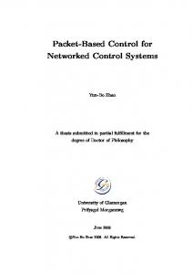
2. Problem Formulation Consider the ILC system with network communication depicted in Figure 1. The discrete time linear plant with actuators and sensors is described by x𝑖 (𝑡+1) = A (𝑡) x𝑖 (𝑡)+B (u𝑖 (𝑡)+w𝑖 (𝑡)) y𝑖 (𝑡) = Cx𝑖 (𝑡) + v𝑖 (𝑡) ,
𝑡 ∈ {0, 1, 2, . . . , 𝑇} , (1)
where 𝑖 ∈ Z+ denotes the iteration index; 𝑇 ∈ Z+ is a given finite time; x𝑖 (𝑡) ∈ R𝑛 , u𝑖 (𝑡) ∈ R𝑞 , and y𝑖 (𝑡) ∈ R𝑚 are state, control, and output, respectively; A(𝑡) ∈ R𝑛×𝑛 is unknown matrix, while B ∈ R𝑛×𝑞 and C ∈ R𝑚×𝑛 are known; w𝑖 (𝑡) ∈ R𝑞 and v𝑖 (𝑡) ∈ R𝑚 are random noises with E[w𝑖 (𝑡)] = 0 and E[v𝑖 (𝑡)] = 0; for all 𝑖 ∈ Z+ , the initial state x𝑖 (0) is a random variable of E[x𝑖 (0)] = x0 with a fixed point x0 ∈ R𝑛 . Assume that CB has full-column rank. The discrete time controller consists of a ILC algorithm and a memory. The controller and the actuators are connected via a communication network through which the controller transmits data to the actuators, while the controller is directly connected to the sensors. The
plant and the controller are assumed to be time driven and synchronized. At each 𝑡 ∈ {0, . . . , 𝑇} of the 𝑖th iteration stage, the con̂ 𝑖 (𝑡) ̂ 𝑖 (𝑡) is computed, the controller transmits u troller output u to the actuators through the network. The transmission may succeed or fail. For a successful transmission, it is assumed that the transmission delay through the network is negligible. With the negligible delay, the actuators can employ u𝑖 (𝑡) = ̂ 𝑖 (𝑡) is transmitted successfully. Of course, when ̂ 𝑖 (𝑡), when u u ̂ 𝑖 (𝑡) and have the transmission fails, the actuators receive no u to employ u𝑖 (𝑡) = u𝑖 (𝑡 − 1) (this paper prescribes u𝑖 (−1) = 0). Overall, the scheme of actuators is ̂ 𝑖 (𝑡) + (1 − 𝛾𝑖 (𝑡)) u𝑖 (𝑡 − 1) , u𝑖 (𝑡) = 𝛾𝑖 (𝑡) u
(2)
where 1, 𝛾𝑖 (𝑡) = { 0,
̂ 𝑖 (𝑡) succeeds, if the transmission of u ̂ 𝑖 (𝑡) fails. if the transmission of u
(3)
Specially, this paper assumes that, for all 𝑖 ∈ Z+ , for all 𝑡 ∈ {0, . . . , 𝑇}, 𝛾𝑖 (𝑡) is a random variable of E[𝛾𝑖 (𝑡)] = 𝛾 with a constant 𝛾 ∈ (0, 1) as well as that 𝛾𝑖 (𝑡1 ) and 𝛾𝑗 (𝑡2 ) are independent either when 𝑖 ≠ 𝑗 or when 𝑡1 ≠ 𝑡2 . In addition, TCP-like protocol is assumed, in which there is an acknowledgment for a successful transmission, and hence the controller has indicators of whether the current controller output is received or not by the actuators. Assumption 1. Given an output reference trajectory y𝑑 (𝑡), which is realizable; that is, there exists a unique desired control input u𝑑 (𝑡) ∈ R𝑞 such that x𝑑 (𝑡 + 1) = A (𝑡) x𝑑 (𝑡) + Bu𝑑 (𝑡) y𝑑 (𝑡) = Cx𝑑 (𝑡) ,
x𝑑 (0) = x0 .
(4)
The purpose of this paper is to design an iterative learning control law for the above plant with network communication such that y𝑖 (𝑡) tracks y𝑑 (𝑡) as closely as possible when 𝑖 is large enough.
3. ILC Algorithms and Convergence Analysis Denote e𝑖 (𝑡) ≜ y𝑑 (𝑡) − y𝑖 (𝑡). The control law is a D-type ILC with average operator that employs updating mechanism: ̂ 𝑖+1 (𝑡) = u
1 𝑖 𝑖+1 𝑖 L ∑e (𝑡 + 1) ∑ u𝑗 (𝑡) + 𝑖 𝑗=1 𝑖 𝑗=1 𝑗
(5)
= A [u𝑖 (𝑡)] + (𝑖 + 1) LA [e𝑖 (𝑡 + 1)] , where the gain matrix L ∈ R𝑞×𝑚 . From (2) and (5), the holdinput scheme with average ILC is expressed as ̂ 𝑖+1 (𝑡) + (1 − 𝛾𝑖+1 (𝑡)) u𝑖+1 (𝑡 − 1) u𝑖+1 (𝑡) = 𝛾𝑖+1 (𝑡) u = 𝛾𝑖+1 (𝑡) (A [u𝑖 (𝑡)] + (𝑖 + 1) LA [e𝑖 (𝑡 + 1)]) + (1 − 𝛾𝑖+1 (𝑡)) u𝑖+1 (𝑡 − 1) . (6)
Journal of Applied Mathematics
3 Buffer
+
w i (t)
vi (t)
+
+
ui (t)
Actuators
Network
yi (t)
Sensors
Acknowledgment
̂ i (t) u yd (t + 1)
+
Plant
ui−1 (t), ui−2 (t), . . .
Iterative learning control algorithm
ui (t)
yi (t)
Memory yi−1 (t + 1), yi−2 (t + 1), . . .
Figure 1: The schematic diagram of the networked control system.
E [Δu𝑖+1 (𝑡 − 2)]
Define the input and state errors
= 𝛾 (E [A [Δu𝑖 (𝑡 − 2)]] − (𝑖 + 1) LE [A [e𝑖 (𝑡 − 1)]]) Δu𝑖+1 (𝑡) ≜ u𝑑 (𝑡) − u𝑖+1 (𝑡) , Δx𝑖+1 (𝑡) ≜ x𝑑 (𝑡) − x𝑖+1 (𝑡) .
+ (1 − 𝛾) (E [Δu𝑖+1 (𝑡 − 3)] + 𝛿 (𝑡 − 2))
(7) .. .
E [Δu𝑖+1 (0)]
And subtracting u𝑑 (𝑡) from both sides of (6) yields
= 𝛾 (E [A [Δu𝑖 (0)]] − (𝑖 + 1) LE [A [e𝑖 (1)]]) Δu𝑖+1 (𝑡) = 𝛾𝑖+1 (𝑡) (A [Δu𝑖 (𝑡)] − (𝑖 + 1) LA [e𝑖 (𝑡 + 1)])
+ (1 − 𝛾) (E [Δu𝑖+1 (−1)] + 𝛿 (0)) = 𝛾 (E [A [Δu𝑖 (0)]] − (𝑖 + 1) LE [A [e𝑖 (1)]])
+ (1 − 𝛾𝑖+1 (𝑡)) (Δu𝑖+1 (𝑡 − 1) + 𝛿 (𝑡)) , (8)
+ (1 − 𝛾) 𝛿 (0) . (10)
where (this paper prescribes u𝑑 (−1) = 0 and hence 𝛿 (0) = u𝑑 (0)) 𝛿 (𝑡) ≜ u𝑑 (𝑡) − u𝑑 (𝑡 − 1). Noticing that 𝛾𝑖+1 (𝑡) is independent of A[Δu𝑖 (𝑡)], A[e𝑖 (𝑡 + 1)] and Δu𝑖+1 (𝑡 − 1) and taking expectation on both sides of (8), we have
The above expression can be arranged later below (this paper 𝑘2 = 0 when 𝑘2 < 𝑘1 ) prescribes ∑𝑘=𝑘 1
𝑡−1
E [Δu𝑖+1 (𝑡)]
𝑘
E [Δu𝑖+1 (𝑡 − 1)] = ∑ 𝛾(1 − 𝛾) E [A [Δu𝑖 (𝑡 − 𝑘 − 1)]] 𝑘=0
= 𝛾 (E [A [Δu𝑖 (𝑡)]] − (𝑖 + 1) LE [A [e𝑖 (𝑡 + 1)]])
𝑡−1
𝑘=0
(9) 𝑡−1
𝑘+1
+ ∑ (1 − 𝛾) Expanding expression (9) from E[Δu𝑖+1 (𝑡 − 1)] to E[Δu𝑖+1 (0)], we have E [Δu𝑖+1 (𝑡 − 1)] = 𝛾 (E [A [Δu𝑖 (𝑡 − 1)]] − (𝑖 + 1) LE [A [e𝑖 (𝑡)]]) + (1 − 𝛾) (E [Δu𝑖+1 (𝑡 − 2)] + 𝛿 (𝑡 − 1)) ,
𝑘
− (𝑖 + 1) L ∑ 𝛾(1 − 𝛾) E [A [e𝑖 (𝑡 − 𝑘)]]
+ (1 − 𝛾) (E [Δu𝑖+1 (𝑡 − 1)] + 𝛿 (𝑡)) .
𝛿 (𝑡 − 𝑘 − 1) .
𝑘=0
(11) From (1) and (4), we have Δx𝑖 (𝑡 + 1) = A (𝑡) Δx𝑖 (𝑡) + B (Δu𝑖 (𝑡) − w𝑖 (𝑡)) e𝑖 (𝑡) = CΔx𝑖 (𝑡) − k𝑖 (𝑡) .
(12)
4
Journal of Applied Mathematics
Taking expectation on both sides of (12) and expanding expression from E[Δx𝑖 (𝑡 + 1)] to E[Δx𝑖 (1)], we obtain
𝑡
𝑘 ≤ 𝛾 max ∑ (1 − 𝛾) E [A [Δu𝑖 ]](𝜆,𝑎) 𝑡∈{0,...,𝑇} 𝑘=0
E [Δx𝑖 (𝑡 + 1)] = A (𝑡) E [Δx𝑖 (𝑡)] + BE [Δu𝑖 (𝑡)] ,
𝑡−𝑘−1
× ∑ 𝑎−(𝜆−1)𝑡 𝑎(𝜆−1)𝜏
E [Δx𝑖 (𝑡)] = A (𝑡 − 1) E [Δx𝑖 (𝑡 − 1)]
𝜏=0
≤ E [A [Δu𝑖 ]](𝜆,𝑎) max 𝛾 𝑡∈{0,...,𝑇}
+ BE [Δu𝑖 (𝑡 − 1)] , .. .
𝑡
−(𝜆−1)𝑘 − 𝑎−(𝜆−1)𝑡 𝑘𝑎 𝑎𝜆−1 − 1
× ∑ (1 − 𝛾) 𝑘=0
E [Δx𝑖 (1)] = A (0) E [Δx𝑖 (0)] + BE [Δu𝑖 (0)] . (13) The above expression can be arranged later (this paper pre2 scribes ∏𝜏𝜏=𝜏 = I when 𝜏2 < 𝜏1 ) 1 𝑡
𝑡
𝑡+1 E [A [Δu𝑖 ]](𝜆,𝑎) 1 − (1 − 𝛾) 𝛾 max 𝑡∈{0,...,𝑇} 1 − (1 − 𝛾) 𝑎𝜆−1 − 1 E [A [Δu𝑖 ]] (𝜆,𝑎) . ≤ 𝑎𝜆−1 − 1 ≤
E [Δx𝑖 (𝑡 + 1)] = ∑ ∏ A (]) BE [Δu𝑖 (𝜏)]
(18)
𝜏=0 ]=𝜏+1
E [A [e𝑖 (𝑡 + 1)]] = CE [A [Δx𝑖 (𝑡 + 1)]] 𝑡
Theorem 3. For the system with network communication described in Section 2 and the iterative learning controller (5), suppose
𝑡
= C ∑ ∏ A (]) BE [A [Δu𝑖 (𝜏)]] . 𝜏=0 ]=𝜏+1
(14)
𝜌 ≜ I − 𝛾LCB < 1.
For any 𝑎 > 1 and any 𝜆 > 1, denote
Then for all A0 , . . . , A𝑇 ∈ R𝑛×𝑛 , for all 𝜖 > 0, there exist 𝑎 > 1 and 𝜆 > 1 such that
−𝜆𝑡 E [A [Δu𝑖 ]](𝜆,𝑎) ≜ max 𝑎 E [A [Δu𝑖 (𝑡)]]2 , 𝑡∈{0,1,...,𝑇} (15) −𝜆𝑡 E [A [e𝑖 ]](𝜆,𝑎) ≜ max 𝑎 E [A [e𝑖 (𝑡)]]2 . 𝑡∈{0,1,...,𝑇}
𝑡−𝑘−1
𝑘=0
𝜏=0
E [A [Δu𝑖 ]](𝜆,𝑎) ≤ . 𝑎𝜆−1 − 1 Proof. From (17), we have 𝑡
𝑘
𝛾 max 𝑎−𝜆𝑡 ∑ (1 − 𝛾) 𝑡∈{0,...,𝑇}
𝑘=0 𝑡−𝑘−1
× ∑ 𝑎𝑡−𝑘−𝜏 E [A [Δu𝑖 (𝜏)]]2 𝜏=0
𝑡
𝑘
≤ 𝛾 max ∑ (1 − 𝛾) 𝑡∈{0,...,𝑇} 𝑡−𝑘−1 𝜏=0
A [Δu𝑖+1 (𝑡)] = = (17)
𝑖 1 (Δu𝑖+1 (𝑡) + ∑ Δu𝑗 (𝑡)) 𝑖+1 𝑗=1
(21)
1 (Δu𝑖+1 (𝑡) + 𝑖A [Δu𝑖 (𝑡)]) . 𝑖+1
Applying the ensemble operator E[⋅] to both sides of (21) and substituting the relationship (8), we can obtain E [A [Δu𝑖+1 (𝑡)]] 1 𝑖 = E [Δu𝑖+1 (𝑡)] + E [A [Δu𝑖 (𝑡)]] 𝑖+1 𝑖+1 𝛾 = (E [A [Δu𝑖 (𝑡)]] − (𝑖 + 1) LE [A [e𝑖 (𝑡 + 1)]]) 𝑖+1 +
1−𝛾 (E [Δu𝑖+1 (𝑡 − 1)] + 𝛿 (𝑡)) 𝑖+1
+
𝑖 E [A [Δu𝑖 (𝑡)]] . 𝑖+1
𝑘=0
× ∑ 𝑎−𝜆𝜏 E [A [Δu𝑖 (𝜏)]]2 𝑎−(𝜆−1)𝑡 𝑎(𝜆−1)𝜏
(20)
Proof. From definition of average operator, note the relation
𝑘 𝛾 max 𝑎−𝜆𝑡 ∑ (1 − 𝛾) ∑ 𝑎𝑡−𝑘−𝜏 E [A [Δu𝑖 (𝜏)]]2 𝑡∈{0,...,𝑇}
lim E [e𝑖 ](𝜆,𝑎) < 𝜖.
𝑖 → ∞
(16)
Lemma 2. For all 𝑎 > 1, for all 𝜆 > 1, and for all 𝑖 ∈ Z+ , 𝑡
(19)
(22)
Journal of Applied Mathematics
5 𝑡−𝑘−1 𝑡−𝑘
Substituting (11) into (22) leads to the following relationship:
× ∑ ∏ A (]) BE [A [Δu𝑖 (𝜏)]] 𝜏=0 ]=𝜏+1
E [A [Δu𝑖+1 (𝑡)]]
𝑡
𝑖+𝛾 E [A [Δu𝑖 (𝑡)]] − 𝛾LE [A [e𝑖 (𝑡 + 1)]] = 𝑖+1
𝑘=0
(24)
𝛾 𝑡−1 𝑘+1 + ∑ (1 − 𝛾) E [A [Δu𝑖 (𝑡 − 𝑘 − 1)]] 𝑖 + 1 𝑘=0 𝑡−1
𝑘+1
− 𝛾L ∑ (1 − 𝛾) 𝑘=0
+ =
where 𝜇𝑖 (𝑡) ≜ (1/(𝑖 + 1)) ∑𝑡𝑘=0 (1 − 𝛾)𝑘+1 𝛿(𝑡 − 𝑘). Next, combining analogous terms on the right hand of (22), we obtain
E [A [e𝑖 (𝑡 − 𝑘)]]
E [A [Δu𝑖+1 (𝑡)]]
1 − 𝛾 𝑡−1 𝑘+1 ( ∑ (1 − 𝛾) 𝛿 (𝑡 − 𝑘 − 1) + 𝛿 (𝑡)) 𝑖 + 1 𝑘=0
=
𝑖+𝛾 𝛾 E [A [Δu𝑖 (𝑡)]] + 𝑖+1 𝑖+1 𝑡−1
𝑘+1
× ∑ (1 − 𝛾) 𝑘=0
𝛾 𝑖+𝛾 E [A [Δu𝑖 (𝑡)]] + 𝑖+1 𝑖+1 𝑡
E [A [Δu𝑖 (𝑡 − 𝑘 − 1)]]
𝑘=1
𝑘
− 𝛾LC ∑ (1 − 𝛾)
𝑘
− 𝛾L ∑ (1 − 𝛾) E [A [e𝑖 (𝑡 − 𝑘 + 1)]]
𝑘=0
𝑘=0
+
𝑘
× ∑ (1 − 𝛾) E [A [Δu𝑖 (𝑡 − 𝑘)]] 𝑡
𝑡
𝑘
− 𝛾LC ∑ (1 − 𝛾) BE [A [Δu𝑖 (𝑡 − 𝑘)]] + 𝜇𝑖 (𝑡) ,
1 𝑡 𝑘+1 ∑ (1 − 𝛾) 𝛿 (𝑡 − 𝑘) . 𝑖 + 1 𝑘=0
𝑡−𝑘−1 𝑡−𝑘
× ∑ ∏ A (]) BE [A [Δu𝑖 (𝜏)]] 𝜏=0 ]=𝜏+1
(23)
𝑡
𝑘
− 𝛾LC ∑ (1 − 𝛾) BE [A [Δu𝑖 (𝑡 − 𝑘)]] Now let us handle the third term on the right hand side of (23); we will express E[A[e𝑖 (𝑡 − 𝑘 + 1)]] with E[A[u𝑖 ]]. Substituting the state error dynamics (14) into (23) leads to the following relationship:
E [A [Δu𝑖+1 (𝑡)]] 𝛾 𝑖+𝛾 E [A [Δu𝑖 (𝑡)]] + = 𝑖+1 𝑖+1 𝑡−1
𝑘+1
× ∑ (1 − 𝛾) 𝑘=0 𝑡
E [A [Δu𝑖 (𝑡 − 𝑘 − 1)]] 𝑘
− 𝛾LC ∑ (1 − 𝛾) 𝑘=0 𝑡−𝑘
𝑘=1
− 𝛾LCBE [A [Δu𝑖 (𝑡)]] + 𝜇𝑖 (𝑡) =(
𝑖+𝛾 I − 𝛾LCB) E [A [Δu𝑖 (𝑡)]] 𝑖+1
+(
𝑡 𝛾 𝑘 I − 𝛾LCB) ∑ (1 − 𝛾) E [A [Δu𝑖 (𝑡 − 𝑘)]] 𝑖+1 𝑘=1 𝑡
𝑘
− 𝛾LC ∑ (1 − 𝛾) 𝑘=0 𝑡−𝑘−1 𝑡−𝑘
× ∑ ∏ A (]) BE [A [Δu𝑖 (𝜏)]] + 𝜇𝑖 (𝑡) . 𝜏=0 ]=𝜏+1
𝑡−𝑘
(25)
× ∑ ∏ A (]) BE [A [Δu𝑖 (𝜏)]] + 𝜇𝑖 (𝑡) 𝜏=0 ]=𝜏+1
=
𝛾 𝑖+𝛾 E [A [Δu𝑖 (𝑡)]] + 𝑖+1 𝑖+1 𝑡
The relationship (25) can be rewritten as follows: E [A [Δu𝑖+1 (𝑡)]]
𝑘
× ∑ (1 − 𝛾) E [A [Δu𝑖 (𝑡 − 𝑘)]] 𝑘=1
𝑡
𝑘
− 𝛾LC ∑ (1 − 𝛾) 𝑘=0
=(
𝑖+𝛾 I − 𝛾LCB) E [A [Δu𝑖 (𝑡)]] 𝑖+1
+(
𝑡−1 𝛾 𝑡−𝜏 I − 𝛾LCB) ∑ (1 − 𝛾) E [A [Δu𝑖 (𝜏)]] 𝑖+1 𝜏=0
6
Journal of Applied Mathematics 𝑡
Combining Lemma 2, (31) and (32) yields
𝑘
− 𝛾LC ∑ (1 − 𝛾)
E [A [Δu𝑖+1 ]](𝜆,𝑎)
𝑘=0 𝑡−𝑘−1 𝑡−𝑘
1 − 𝛾 𝛾 ‖LCB‖ + 𝛾 + ‖LC‖ ‖B‖ + ) 𝑖+1 𝑎𝜆−1 − 1 × E [A [Δu𝑖 (𝑡)]](𝜆,𝑎) + 𝛼.
× ∑ ∏ A (]) BE [A [Δu𝑖 (𝜏)]] + 𝜇𝑖 (𝑡) .
≤ (𝜌 +
𝜏=0 ]=𝜏+1
(26) To simplify expression of ((𝑖+𝛾)/(𝑖+1))I−𝛾LCB, (𝛾/(𝑖+1))I− 𝛾LCB, and 𝛾LC ∑𝑡𝑘=0 (1 − 𝛾)𝑘 , we choose 𝑎 > 1 and 𝜆 > 1 such that 𝑎 > ‖A (])‖
∀] ∈ {0, . . . , 𝑇} ,
𝛾 ‖LCB‖ + 𝛾 + ‖LC‖ ‖B‖ 1 − 𝜌 , < 4 𝑎𝜆−1 − 1 ‖C‖ ‖B‖
1 𝑎𝜆−1
2𝛼 < 𝜖, −11−𝜌
(27) (28)
There exists 𝑀 ∈ Z+ such that (1 − 𝛾)/(𝑖+ 1) < (1 − 𝜌)/4 when 𝑖 ≥ 𝑀. Now for 𝑖 > 𝑀, (28) and (33) imply that 1 + 𝜌 E [A [Δu𝑖+1 ]](𝜆,𝑎) ≤ E [A [Δu𝑖 ]](𝜆,𝑎) + 𝛼, 2 E [A [Δu𝑖+1 ]](𝜆,𝑎) ≤(
(29)
1 + 𝜌 𝑖+1−𝑀 ) E [A [Δu𝑀]](𝜆,𝑎) 2 𝑖−𝑀
+ ∑(
where
𝑗=0
𝑎−𝜆𝑡 𝑡 𝑘+1 ∑ (1 − 𝛾) ‖𝛿 (𝑡 − 𝑘)‖2 𝑡∈{0,...,𝑇} 2 𝑘=0
≤(
𝛼 ≜ max
𝜇𝑖 (𝑡)2 .
−𝜆𝑡
≥ max 𝑎 𝑡∈{0,...,𝑇}
(30)
1+𝜌 𝑗 )𝛼 2
1 + 𝜌 𝑖+1−𝑀 ) E [A [Δu𝑀]](𝜆,𝑎) 2 𝑖+1−𝑀
+
1 − ((1 + 𝜌) /2) 1 − ((1 + 𝜌) /2)
𝛼. (34)
Taking 𝜆-norm on both sides of (26), we obtain Consequently, we obtain
E [A [Δu𝑖+1 ]](𝜆,𝑎) 1 − 𝛾 ≤ I − 𝛾LCB − I E [A [Δu𝑖 ]](𝜆,𝑎) 𝑖 + 1 + max 𝑎−𝜆𝑡 𝜇𝑖 (𝑡)2 𝑡∈{0,...,𝑇}
2𝛼 . lim E [A [Δu𝑖+1 ]](𝜆,𝑎) ≤ 1−𝜌
𝑖 → ∞
𝑡−1
𝑡−1 𝑡−1
E [A [e𝑖 (𝑡)]] = C ∑ ∏ A (]) BE [A [Δu𝑖 (𝜏)]] . Similar to the proof of Lemma 2, one can prove that
E [A [Δu𝑖 (𝜏)]]2
max 𝑎−𝜆𝑡 E [A [e𝑖 (𝑡)]]2
𝑡∈{0,...,𝑇}
+ 𝛾 ‖LC‖ ‖B‖ max 𝑎−𝜆𝑡 𝑡∈{0,...,𝑇}
𝑡−1
≤ ‖C‖ ‖B‖ max 𝑎−𝜆𝑡 ∑ 𝑎𝑡−1−𝜏 E [A [Δu𝑖 ]]2
𝑡−𝑘−1
𝑡
𝑡∈{0,...,𝑇}
𝑘 × ∑ (1 − 𝛾) ∑ 𝑎𝑡−𝑘−𝜏 E [A [Δu𝑖 (𝜏)]]2 . 𝜏=0
𝑘=0
(31) Using Lemma 2, it can be proved that, for all, 𝑎 > 1, for all 𝜆 > 1, and for all 𝑖 ∈ Z+ , 𝑡−1
𝑡∈{0,...,𝑇}
𝜏=0
E [A [Δu𝑖 ]](𝜆,𝑎) ≤ . 𝑎𝜆−1 − 1
𝜏=0
E [A [Δu𝑖 ]](𝜆,𝑎) . ≤ ‖C‖ ‖B‖ 𝑎𝜆−1 − 1
(37)
Finally, from (29), (35), and (37), we can obtain 1 2𝛼 lim E [A [e𝑖+1 ]](𝜆,𝑎) ≤ ‖C‖ ‖B‖