On large data sets the import process can take ...

NASA/TM—2000-210065

PSIDDIII: Post-Scan Ultrasonic Data Display System for the Windows-Based PC Including Fuzzy Logic Analysis

Jeffrey J. Lovelace and Krzysztof J. Cios University of Toledo, Toledo, Ohio Don J. Roth Glenn Research Center, Cleveland, Ohio Wei Cao West Virginia University, Montgomery, West Virginia

June 2000

The NASA STI Program Office . . . in Profile Since its founding, NASA has been dedicated to the advancement of aeronautics and space science. The NASA Scientific and Technical Information (STI) Program Office plays a key part in helping NASA maintain this important role.

•

CONFERENCE PUBLICATION. Collected papers from scientific and technical conferences, symposia, seminars, or other meetings sponsored or cosponsored by NASA.

The NASA STI Program Office is operated by Langley Research Center, the Lead Center for NASA’s scientific and technical information. The NASA STI Program Office provides access to the NASA STI Database, the largest collection of aeronautical and space science STI in the world. The Program Office is also NASA’s institutional mechanism for disseminating the results of its research and development activities. These results are published by NASA in the NASA STI Report Series, which includes the following report types:

•

SPECIAL PUBLICATION. Scientific, technical, or historical information from NASA programs, projects, and missions, often concerned with subjects having substantial public interest.

•

TECHNICAL TRANSLATION. Englishlanguage translations of foreign scientific and technical material pertinent to NASA’s mission.

•

•

•

TECHNICAL PUBLICATION. Reports of completed research or a major significant phase of research that present the results of NASA programs and include extensive data or theoretical analysis. Includes compilations of significant scientific and technical data and information deemed to be of continuing reference value. NASA’s counterpart of peerreviewed formal professional papers but has less stringent limitations on manuscript length and extent of graphic presentations. TECHNICAL MEMORANDUM. Scientific and technical findings that are preliminary or of specialized interest, e.g., quick release reports, working papers, and bibliographies that contain minimal annotation. Does not contain extensive analysis. CONTRACTOR REPORT. Scientific and technical findings by NASA-sponsored contractors and grantees.

Specialized services that complement the STI Program Office’s diverse offerings include creating custom thesauri, building customized data bases, organizing and publishing research results . . . even providing videos. For more information about the NASA STI Program Office, see the following: •

Access the NASA STI Program Home Page at http://www.sti.nasa.gov

•

E-mail your question via the Internet to [email protected]

•

Fax your question to the NASA Access Help Desk at (301) 621-0134

•

Telephone the NASA Access Help Desk at (301) 621-0390

•

Write to: NASA Access Help Desk NASA Center for AeroSpace Information 7121 Standard Drive Hanover, MD 21076

NASA/TM—2000-210065

PSIDDIII: Post-Scan Ultrasonic Data Display System for the Windows-Based PC Including Fuzzy Logic Analysis

Jeffrey J. Lovelace and Krzysztof J. Cios University of Toledo, Toledo, Ohio Don J. Roth Glenn Research Center, Cleveland, Ohio Wei Cao West Virginia University, Montgomery, West Virginia

National Aeronautics and Space Administration Glenn Research Center

June 2000

Available from NASA Center for Aerospace Information 7121 Standard Drive Hanover, MD 21076 Price Code: A04

National Technical Information Service 5285 Port Royal Road Springfield, VA 22100 Price Code: A04

Table of Contents Key to Special Notations ........................................................................................................... iv PSIDD III – Background ................................................................................................................ 1 History......................................................................................................................................... 1 Software Strategy........................................................................................................................ 1 Fuzzy Logic Image Analysis ...................................................................................................... 2 Ultrasonic Contact Measurement Method .................................................................................. 3 PSIDD III – Common Tasks........................................................................................................... 4 Installing the Program................................................................................................................. 4 PSIDD Screen Layout................................................................................................................. 4 When PSIDD Starts .................................................................................................................... 5 Step 1 - Display the PSIDD Splash Screen............................................................................. 5 Step 2 - See if the Local Interbase Server is Running ............................................................ 5 Step 3 - See if the user has run PSIDD before........................................................................ 6 Step 4 - Process the PSIDD.INI file........................................................................................ 7 Step 5 - Finishing Up .............................................................................................................. 7 Importing a Data Set ................................................................................................................... 7 Importing VAX Raw Data ...................................................................................................... 7 Importing PC Raw Data.......................................................................................................... 8 Opening a File........................................................................................................................... 10 Selecting Points on an Image.................................................................................................... 10 Graphing Points ........................................................................................................................ 11 Printing Options ........................................................................................................................ 11 Selecting a Different Image ...................................................................................................... 11 Modifying Image Data.............................................................................................................. 12 Adding New Data to an Existing Database to Facilitate Comparative Analysis...................... 13 Creating Sequence of Images to use in a Movie....................................................................... 13 Creating a New Graph .............................................................................................................. 14 Creating a New Graph Format ini File ..................................................................................... 14 Menu Structure and Functions .................................................................................................. 14 PSIDD III – Windows and Dialog Boxes ..................................................................................... 17 Main Window ........................................................................................................................... 17 Dialog Boxes Associated with the Main Window.................................................................... 18 Import Files Dialog Box ....................................................................................................... 18 Location of Files Dialog Box................................................................................................ 18 Import Files Dialog Box ....................................................................................................... 19 Expand Frequency Range Dialog Box.................................................................................. 20 Printing Options Dialog Box ................................................................................................ 21 Image Window.......................................................................................................................... 22 Dialog Boxes Associated with the Image Window .................................................................. 23 Image Type Dialog Box........................................................................................................ 23 Image Color Options Dialog Box ......................................................................................... 24 Modify Image Dialog Box .................................................................................................... 25 Histogram Window................................................................................................................... 26

NASA/TM—2000-210065

iii

Arial View Window.................................................................................................................. 26 Graph Window.......................................................................................................................... 27 Dialog Boxes Associated with the Graph Window .................................................................. 28 Graph Settings Dialog Box ................................................................................................... 28 Graph Properties Dialog Box................................................................................................ 29 PSIDD III – Programmer Reference............................................................................................. 30 Registry Entries......................................................................................................................... 30 INI File formats......................................................................................................................... 32 PSIDD INI Format................................................................................................................ 32 Graph INI Format ................................................................................................................. 34 Installations ............................................................................................................................... 35 Online Help............................................................................................................................... 35 Printing Details ......................................................................................................................... 35 Functional Overview................................................................................................................. 36 Database Structure .................................................................................................................... 36 Source Code .............................................................................................................................. 37 Primary Objects .................................................................................................................... 37 Form Units ............................................................................................................................ 38 Helper Units .......................................................................................................................... 39 Global Variables ................................................................................................................... 39 Help File Creation..................................................................................................................... 39 Compiling New Versions of PSIDD......................................................................................... 40 Creating an Installation Routine ............................................................................................... 40 Appendix A: Detailed Example of how to add points to an existing database............................. 41 Part 1: Creating a new database ................................................................................................ 41 Part 2: Adding another Data Point to the existing Database file .............................................. 44 Part 3: Modifying the Image to Display the new Data Points .................................................. 47 References..................................................................................................................................... 50

1

Key to Special Notations

á L 0

&

This indicates a dangerous element that should be carried out by someone that knows exactly what they are doing and understand the ramifications of the change. This indicates potential differences between Windows NT and Windows 9X when PSIDD is run. This indicates which group of people should read a section. This indicates a warning that the operation of a function is one way and will not be able to be undone with out importing the raw data again. This indicates a helpful tip to the user.

NASA/TM—2000-210065

iv

Abstract Post-Scan Interactive Data Display (PSIDD) III is a user-oriented Windows-based system that facilitates the display and comparison of ultrasonic contact data. The system is optimized to compare ultrasonic measurements made at different locations within a material or at different stages of material degradation. PSIDD III provides complete analysis of the primary wave forms in the time and frequency domains along with the calculation of several frequency dependent properties including Phase Velocity and Attenuation Coefficient and several frequency independent properties, like the Cross Correlation Velocity. The system allows image generation on all of the frequency dependent properties at any available frequency (limited by the bandwidth used in the scans) and on any of the frequency independent properties. From ultrasonic contact scans, areas of interest on an image can be studied with regard to underlying raw waveforms and derived ultrasonic properties by simply selecting the point on the image. The system offers various modes of in-depth comparison between scan points. Up to five scan points can be selected for comparative analysis at once. The system was developed with Borland Delphi software (Visual Pascal) and is based on a SQL database. It is ideal for classification of material properties, or location of microstructure variations in materials.

NASA/TM—2000-210065

v

PSIDD III – Background

L

Individuals who are interested in learning about the development of the PSIDD system and the type of ultrasound data that it is designed to analyze should read this section.

History In 1992, NASA Glenn (Lewis) researchers developed the Post-Scan Interactive Data Display (PSIDD) system [1], a system that was optimized for viewing ultrasonic contact scan data. Originally, PSIDD was designed to show images from ultrasonic contact scans and allow only one scan location to be viewed for further analysis. In 1996, PSIDD II [2] evolved to allowed a user to select up to five scan locations at one time for comparative analysis. Both of these versions were developed on the DEC VAX with the aid of a Grinnell image processing system for graphics. The source code was all written in Fortran. Although functional, the system had several inconveniences. First, users were forced to use a dual monitor system (commands entered on the VAX terminal and graphic operations performed on the image processing system monitor). Additionally, the image processing system required commands to be entered by moving a cursor and setting a series of switches on a cursor control unit attached to the image processor. This made the system cumbersome to use because it was difficult to remember the correct sequence of switches to get the desired results. Further, the graphs were forced to appear in one of two modes. Information on the image processing system monitor was also difficult to transfer to an image format to include results in reports. Waveform data was stored in multiple files with different proprietary formats making it difficult to get data from PSIDD to another program for further analysis. Finally, the VAX-based system was expensive to buy and was not very portable. This meant that for anyone wishing to analyze some data acquired by means of ultrasound contact scanning, that individual would have be required to visit NASA Glenn Research Center. To overcome these issues it was decided to port the entire system to Windows running on an IBM-compatible personal computer (PC). PSIDD III would enjoy the benefits of a graphically oriented environment. This would allow information to be seamlessly passed between PSIDD and other systems for reporting or presentation use. Also, the interface would be much simpler for the end user by replacing the original cursor control unit with a mouse. PSIDD III has been developed jointly between NASA Glenn and the University of Toledo. Although the system had to emulate the existing user display and functionality, the entire system was redesigned from the ground up. Software Strategy The foundation for the new system is storing of all data within a SQL database structure. In order to speed up development the entire system was coded in the Delphi environment. Delphi is an Object Oriented Programming (OOP) environment based on Pascal to provide Rapid Application Development (RAD) that is designed specifically to speed the development of database software packages in the Windows environment. Delphi allows for the quick creation of professional software packages in minimal amount of time. It accomplishes this task by insulating the user from the complex

NASA/TM—2000-210065

1

windows environment with a suite of OPP graphical user interface and database connectivity components. This allows the user to develop the interface and the logic quickly. Since the entire package is OOP, it is possible to work at the Windows Application Programming Interface (API) level or ignore its function all together. The final benefit is the ability to derive new classes by inheriting and modifying an existing class to enhance or add functionality. Essentially, PSIDD acts an interpreter between the user and the database system to retrieve, process, and display appropriate information to the user. Storing information in the database makes all data available to other Windows programs directly through Open DataBase Connectivity (ODBC). ODBC is a standard Application Programming Interface (API) that allows a program to communicate to a database, which is independent of the type of database. This system is designed to work with data collected by the ultrasonic contact measurement method developed at NASA Glenn [3]. It can import previously-obtained data from the VAXbased scan system for analysis or analyze new data obtained from a PC-WindowsLabview-based ultrasonic measurement system recently developed at NASA Glenn [5]. The PSIDD system has been presented at the American Society for Nondestructive Testing Annual Conference [7]. Fuzzy Logic Image Analysis One of the benefits of the new system is the incorporation of a fuzzy image analysis algorithm that attempts to locate areas of interest on the image. There are 256 colors generated for each image by PSIDD. The colors are equally spaced on the image from the lowest value to the highest value. The fuzzy analysis is based on this 256-color scheme. The system attempts to answer the following question for a scan location: Is my intensity atypical and is my local intensity difference very high? If the answer to this question is yes, than the point is flagged as interesting. In the fuzzy world, this statement is evaluated to the degree to which it is true, in the range from 0 to 1. To perform this calculation requires the formation of two fuzzy sets. The first fuzzy set is that of atypical intensity. The atypical intensity fuzzy set is calculated by generating a histogram of the colors used in the image. The histogram is normalized to 1. The value for each bin is subtracted from 1. In this fashion, the most common colors in the image will have a fuzzy membership value that is low or close to zero while colors that appear sparsely in the image will have a high membership value. The other fuzzy set is local intensity difference. This fuzzy set is first calculated by determining the minimum intensity difference between a scan location and up to its eight nearest neighbors for each scan location. These results are then put into a histogram with bins ranging from 0 to 255 units of intensity difference. The histogram is then normalized to 1. Next the value of each bin is subtracted from 1. In this way, a fuzzy set is generated that will assign low membership values to points with very little intensity difference and high values to large intensity differences. In a fuzzy and operation the smallest of the two values is used as the result. In order to obtain a high membership for the rule both sets must also have high membership values. It is up to the user to define a threshold at which the system will actually flag a particular point. This implementation is primarily based on the work of Sacha, Cios, Roth, et al. [4].

NASA/TM—2000-210065

2

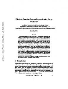
Ultrasonic Contact Measurement Method This NASA Glenn ultrasonic contact measurement method involves digitizing four waveforms for a scan location on a sample. Figure 1 shows a layout of the data collection system and the waveforms. During an automated ultrasonic contact scan, a sample is divided into a grid of measurements and at each scan location on the grid, the four waveforms are stored for further analysis. Alternately, manual measurements at a variety of locations across a sample or during various stages of degradation of the sample can be performed and the waveforms subsequently stored.

Figure 1: Ultrasonic Contact Measurement Method. (a) Diagram of buffer rod-couplant-sample pulse-echo contact configuration. FS2(T) front surface reflection. B1(T) =first back-surface reflection. B2(T) second back-surface reflection. FS1(T), not shown in this figure but shown in upcoming waveform displays, is acquired without sample or couplant on buffer rod. (b) Resulting waveforms for pulse-echo contact technique. (c) Schematic (top view) of ultrasonic contact scan procedure showing examples of successive transducer positions along X- and Ydimensions of sample

The analysis system calculates the Fourier transform of all four signals. From the time and frequency-domain Fourier data, the following frequency based information is determined: For Each Waveform: Magnitude Phase Power (only for PC-Windows-Labview system) slew rate (only for PC-Windows-Labview system) risetime (only for PC-Windows-Labview system) falltime (only for PC-Windows-Labview system) overshoot (only for PC-Windows-Labview system) pulse width [usec] (only for PC-Windows-Labview system) NASA/TM—2000-210065

3

-6db magnitude spectra width magnitude spectra peak frequency Area under power spectra curve For Each Scan Location: Reflection Coefficient Attenuation Coefficient % Attenuation Coefficient Error Phase Velocity Cross Correlation Velocity The calculations used to obtain these values can be found in [2].

PSIDD III – Common Tasks

L

This section describes how common tasks within PSIDD can be accomplished. It is for a user who needs to get the basics for PSIDD and wants to use the program but does not need to know the in-depth functioning of the program. Elements within {}'s are dialog boxes that are described in detail in the PSIDD III - Dialog Boxes section.

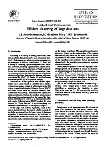
Installing the Program PSIDD is installed by running setup.exe from the setup directory. The system requires at least 32 Mb of memory for PSIDD to run smoothly. PSIDD Screen Layout The typical screen elements in available when the PSIDD application is started are shown in Figure 2. Those elements are: A: Main Menu Window – Contains speed buttons to accelerate features found in the menus. The user can also toggle smoothing, grid overlay, and good bad data overlay on the image. The current scan location is also indicated. B: Image Window – The user can choose which points he wishes to investigate further by simply pushing the mouse button when it is over the proper position. Multiple points are selected or deselected by holding the shift key while pushing the mouse button. The image window will also list the Data Point Id and location of each point in the upper right hand corner of the image window. At the bottom of the image window, a legend for the colormap shows the high, low, and average value (triangle) for the current image. Note that a series of manual measurements made across a sample, or measurements made at a single location as a function of time, can also be displayed as an image. C: Graph Window – The graph window shows the data for a property or waveform. Up to two different properties can be displayed on the same graph. Only properties with a similar scale are allowed on the same graph (Time or Frequency). Up to five data points showing values for the same property can be displayed on one graph.

NASA/TM—2000-210065

4

Right clicking on a graph window brings up a menu that allows the user to copy the graph to the clipboard or to a file. D: Arial View – The arial view shows the user selections exaggerated on a small image. The color-coding of the dots is the same as the colors used to represent those data points on the graphs. The arial view comes up automatically any time the image window is minimized. Double Clicking on the arial view will bring the image window to the front. E: Histogram – The histogram window allows the user to see how the colors in the image are distributed. The user can select regions to expand the histogram about. Points outside the region are nearest neighbor filtered or marked with a color indicating that they were above or below the cut off level.

Figure 2: PSIDD Screen Elements

When PSIDD Starts Whenever PSIDD is run by a user it goes through a five step process to fully start up to a point where users can use the application. Those steps are described in detail below. Step 1 - Display the PSIDD Splash Screen During initialization PSIDD displays a splash screen indicating that this project was a joint effort between NASA and the University of Toledo. Step 2 - See if the Local Interbase Server is Running Interbase is the database engine that PSIDD uses to store and retrieve data about a given data set. The program looks for the Interbase process in the list of current process NASA/TM—2000-210065

5

running on the system to determine if the Interbase server has been started. If the server is not started the system will look up its location in the Window's Registry and try to start it. The Window's Registry is a common location in the Windows environment to store application data.

á

1

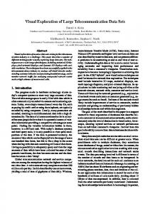
On Windows NT, the installation program may not make the correct changes to the Registry so that PSIDD can locate the Interbase Server. In this case the server must be set to always run or must be started manually before PSIDD is run. If PSIDD cannot detect the presence of the Interbase server it will stop loading at this point and exit. Step 3 - See if the user has run PSIDD before In this phase of start up PSIDD will check to see if this user has used PSIDD before. It accomplishes this task by checking the Registry. If the person has used PSIDD before their previous values will be automatically loaded up. If this is the first time the user has started PSIDD, default values will be selected for the user and the user will be given a chance to change or keep these values. The default values should work for most users. On line help is available by pressing F1 when the dialog box is active. The {Location of Files} dialog box will allow the user to change these settings. It is shown in Figure 3.

á 0

On Windows NT, the installation program may not make the correct changes to the Registry, if this is the case all of fields will begin with "C:\". The user will have to manually select the right locations. If the settings are wrong PSIDD may experience random errors like not being able to open up existing files or create new files.

Figure 3: PSIDD Location of Files Dialog Box

NASA/TM—2000-210065

6

Step 4 - Process the PSIDD.INI file The PSIDD.INI file contains information about what types of waveforms may be available in different data sets and how that data should be imported. As this file is processed the user will see a red progress indicator on the splash screen fill up.

0

If the bar does not show up read the section on the {Location of Files} dialog box and verify that all of the locations are correct. Step 5 - Finishing Up After correctly passing the previous steps PSIDD will display an empty image window and hide the splash screen. PSIDD is now ready for use.

Importing a Data Set The first task a user will need to do is convert the raw data into a format that PSIDD can use to work with. This is accomplished by selecting FileÆImport from the menu. This will cause the {Import Files} dialog box to appear. On line help is available for the {Import Files} dialog box by pushing F1. Currently PSIDD supports importing two different types of raw data. The first is data that was created on the VAX and the second is data that was created under the PC-Windows-Labview system.

&

On large data sets the import process can take upwards of 1 hour. Importing VAX Raw Data There are two different paths that are used when importing files. This is a 4-step process. Importing files for the VAX is done with a two step process. Step 1 - Select the PSIDD VAX Files tab The {Import File} dialog box consists of two tabs one for VAX and one for PC raw data. Select the tab for PSIDD VAX Files. Figure 4 shows how this tab should appear.

Figure 4: Import Files dialog box

NASA/TM—2000-210065

7

Step 2 - Fill in the Data File Names There are 6 files that need to be specified before the Import button will become available, they are: *.datwav *.dati2 *.datr4 *.datGB *.spc *.spcinfo

This file contains all of the digitized waveforms. This file contains 16bit integers for various system parameter settings. This file contains 4 byte floating point numbers of time offsets (time window start position). This file contains the good/bad data information. This file contains the digitized spectral data. This is a header file for the spc file.

The user can either manually enter each of the fields or use the browse button to select the files from a File Selection dialog box. PSIDD automatically detects the need for the *.daths file (h = holder: no ultrasonic data taken, s = sample: data taken) created during VAX-based scans. PSIDD will look for it within the directory where the other files are located using the naming convention of the existing files to determine which *.daths file is the right one if there happens to be more than one. Step 3 - Selecting a Database Name After entering the file names the user can select Import. After pressing Import, the user will be prompted to enter a name for the database. This will be the file the user will use to access this data in the future. If the name is valid PSIDD will begin the Import process. Step 4 - Importing the Data During the Import the status bars at the lower left will indicate how much of the total import is complete for the current point and for all of the points. At the right hand side there is a status area that shows current information. Importing PC Raw Data Importing raw data collected on the PC-Windows-Labview system offers a few options not available for data obtained on the VAX-based system. NOTE: It is possible to add a newly collected data sample from the PC-Windows-Labview system to an existing database or create a new database. Importing PC based data is a 5-step process. Step 1 - Selecting the Type of Import There are two types of import that PSIDD can do with a PC acquired data. The first is to create an entirely new database file. The other option is to add a new data point to an existing database file. To add a point the new data set must match the number of digitized records per waveform. This step is shown in Figure 5.

0

To successfully add data points to an existing data set, the number of digitized points, sample frequency and time window widths of all four waveforms must match.

NASA/TM—2000-210065

8

Figure 5: Step 1 – Importing PC based files

Step 2 - Selecting the Files The PC-collected files consist of two files. The first is the header file (*.hed). The header file contains information about the sample that is not specific to a particular point. The second is the data file (*.dat). It contains all of the information about the digitized waveforms and other calculations done at each sample location. Both of these files are comma separated and can be opened in a wide variety of spreadsheet programs. Step 2 is shown in Figure 6.

Figure 6: Step 2 – Importing PC based files

Step 3 - Selecting the Database File Step 3 involves selecting the database file. If the user’s choice was to add to an existing database then a browse button is available that allows the user to pick the database file. If it is the case where a new database file will be created, the user must type in the name of a new file to be created. For the latter, the user simply types in the name of the new database. Figure 7 shows the case for a new database.

NASA/TM—2000-210065

9

Figure 7: Step 3 – Importing PC based files

Step 4 - Importing the data Step 4 is when PSIDD performs the data import. Pressing the import button starts the process. During an import, status information is displayed on the dialog box. In formation about each location that was scanned for a given data set is stored sequentially. PSIDD imports the data by loading one location at a time. If the import action is an addition to an existing set, the points are added sequentially at the back of the table. Step 5 - Modifying the Image Data to Display the New Points Step 5 is only required when one data set is added to another. PSIDD needs to be told where the new point(s) should be shown on the existing image. This is accomplished by opening the database and selecting ImageÆModify Image from the menu. The {Modify Image} dialog box is discussed in detail in Windows and Dialog Boxes section. Opening a File To open a database file, select File->Open. This will cause the file open dialog box to appear that is common to all windows applications. The user can open any previously created database file (*.gdb). After the file opens successfully the Image Window will appear similar to Figure 8. The speed buttons and menu options should all be enabled. Selecting Points on an Image Points are selected on the image by pressing the left mouse button when the mouse is over an area of the image that has data. Multiple point can be selected by holding down the shift key while pressing the left mouse button. Point can be unselected by selecting them with the mouse again. As points are selected they are added to the selected points list to the right of the image.

NASA/TM—2000-210065

10

Figure 8: Image Window

Graphing Points To graph points that have been selected on the Image Window the user simply selects the graph points speed button on the {Main Window}. The system will then collect information about each point and display a graph corresponding to different waveform or calculated properties. The graph windows can be adjusted independently. The options for the {Graph Window} are discussed in more detail in the Windows and Dialog Boxes section. Printing Options If desired a hard copy of all of the graphs and the image window can be sent to a printer. The report can be printed by selecting FileÆPrint from the menu. On line help is available for the {Printing Options} dialog box by pressing F1. Selecting a Different Image PSIDD forms images by looking at the values for a scan point or waveform property (possibly at a specific frequency if the property is frequency-based) for all sampled locations. It then finds the highest and the lowest values. Next it creates a 256 level linear color scale by normalizing the data based on the high and low value. To draw the image it assigns each point a color based on its value. A new image can be generated by selecting Image->Image Type from the menu. The {Image Selection From} dialog box is shown in Figure 9. It allows the user to select which image to display.

NASA/TM—2000-210065

11

Figure 9: Image Selection Form

Modifying Image Data Modifying image data is available to allow the user to reposition points on the image for an easy evaluation of the data that was collected. Primarily it is intended for the case where the user has decided to do a batch process where one or more points is collected from a large number of samples and the information is to be studied side by side. Additionally, it can be used in the case where the user is performing a time study on one sample through some extended test and wants to see the results side by side. It is to be used in conjunction with the addition of points import to add the new points to the image information. It is accessed through the ImageÆModify Image menu. The work is performed in the {Modify Image} dialog box. This tool allows the user to modify any aspect of the image including size, shape, and number of points. It can be used with any database. To add points to an image the user simply drags an unassigned Data Point Id to the image diagram as shown in Figure 10. Pressing OK will change the database to match the new configuration. On line help is available for the {Modify Image} dialog box by pressing F1.

0

Modifying the image is a powerful feature but once the changes are made there is no automatic way to return the image to its original state. The user has to manually undo the changes they made by calling the Modify Image menu command again.

Figure 10: Modify Image dialog box

NASA/TM—2000-210065

12

Adding New Data to an Existing Database to Facilitate Comparative Analysis One of the new features this version of PSIDD offers is the ability to add data points to existing data sets. This process can only be carried out under special circumstances. Those circumstances are: 1. The data must be collected with the PC-Base software. 2. Identical collection parameters must be specified current and new data sets (Digital Samples per Waveform, and Frequency Interpolation Interval). The procedure is fairly simple. Step 1 – Collect the new data The collection must be done with the exact same parameters as used in the data set the user will add this data set to. Step 2 – Add the new data to the existing data set New data is added to an existing data set. This is accomplished through the import menu. In step 1, the user should select “Add Data Points to an Existing Database”. Follow the rest of the steps to get PSIDD to add the new data to the database file. PSIDD will add the new data in the order that they appear in the file. The data point id’s will be incremented sequentially. Step 3 – Modify the Image to display the new data point(s) Open up the database in PSIDD. Select “Modify Image” from the Image menu. The new data points that have been added to the database file will be listed by data point id in the unassigned id box. The user must drag the id’s to locations on the image. For more detailed direction see the section on Modifying Image Data in the Common tasks section of this manual. The idea behind this feature is to allow the user to perform two types of studies. The first would be the analysis of a batch of physically identical samples but with perhaps different microstructure characteristics. The other would be the collection and analysis of a single sample as it goes through a series of tests over a period of time. Creating Sequence of Images to use in a Movie One of the final features of PSIDD is the ability to generate a sequence of images for a frequency-dependent property that can be used to create an animation sequence. This is accomplished by selecting File->Make Movie Frames from the menus. The Create Movie Frames dialog box will be displayed (shown in Figure 11). The user must select a frequency based property to form the image on, pick how large (in pixels) each data point will be, toggle smoothing, set a Max value for the legend, set a Min value for the legend, and finally pick a directory to store the images in. The directory must be one that does not exist. To pick a good value for the Max and Min values the user should look at graph of the particular property with several points selected. Since this process may be lengthy, a status area with a percent complete indicator is located in the bottom

NASA/TM—2000-210065

13

left corner. The number of images is equal to the number of digitized locations for the frequency based property that the images are being generated for. The images are stored as Window’s bitmap files and can be converted into a variety of animation formats with the appropriate software.

Figure 11: Create Movie Frames Dialog Box

Creating a New Graph It may be possible that the default series of graphs that PSIDD displays may not contain the graph of a desired property. In that case the user can select Windows->New Graph… from the menu. This will generate a new {Graph Window} and display its {Graph Properties} dialog box so the user can draw the graph they want. When they press “OK” a new graph will be drawn according to the graph properties that were selected. Creating a New Graph Format ini File To capture the current status of all of the graph windows and save that to a form PSIDD can use to recreate the sequence, all the user has to do is select Windows->Save Locations. To make this configuration the default for either multiple point or single point graphs, change the value of the appropriate edit box in the {Location of Files} dialog box located under Settings->File Locations on the menus. Menu Structure and Functions File Menu Open Import Print Expand Frequency

Used to perform file operations Used to select and open a database file Used to import raw data into a database file Used to send reporting information to the printer Performs a cubic spline interpolation to increase the resolution of the frequency data.

Make Movie Frames Used to create a sequence of images that can be used to make an animation sequence. Clear Image Cache

NASA/TM—2000-210065

Clear the image cache table from the database file. This command should only be run if the time to recall a previous image seems much longer than normal.

14

Exit Image Menu Graph Points Image Type

Colors

Histogram

Arial View

Modify Image

Save Image Settings Menu Graphs

File Locations

Windows Menu Image to Front Align Image Graphs to Front Graphs Image New Graph

NASA/TM—2000-210065

Exits the program. Used to perform image operations Graph the currently selected points. Select which image to display and at what frequency. Causes the Image Selection Form dialog box to appear. This form is discussed in further detail in the Image Window section. Select color style and patterns used in the image as well as filtering options. Causes the Image Color Options dialog box to appear. This dialog is discussed in further detail in the Image Window section. Display image histogram information. The histogram is used to expand the image color scale around values of interest in the image. The histogram and its uses are discussed further under the Image Window section. Display an always on top small version of the Image Window with the selected points color-coded to match the graphs. Activates the Modify Image dialog box. This allows the user to add data points to a previous data set, remove points from an image, and/or restructure the format of an existing image. This is a very powerful feature and if used in correctly can render a database file useless and it will have to be rebuilt from the raw data again. Save the current image and legend to a bitmap file. Used to adjust the global application settings Adjust the graph settings. This causes the Graph Settings dialog box to appear. It changes settings to all of the graphs currently on the screen or graphs that will be generated in the future. Used to adjust the file location start up information. Causes the File Location dialog box to be displayed (Figure 3). See the beginning of the running PSIDD for the first time section for more information on this item. Used to arrange the image and graph windows Bring the image window to the front of the display. Resize to the default size and bring the image window to the front of the display. Brings the graph windows to the front of the display. Resizes the graphs to their original size and position and bring the graphs to the front of the display. Creates and new graph and adds it to the end of the list of graphs.

15

Save Locations

Help Menu Contents About

NASA/TM—2000-210065

Creates a new graph ini based on the current graph positions. Used to access on line help system Displays the online help table of contents. Displays the PSIDD splash screen. Clicking anywhere in the image will make it disappear.

16

PSIDD III – Windows and Dialog Boxes

L

This section describes details for each of PSIDD's windows and dialog boxes. Users who need to know all of the functions that are available for each window or dialog box should read it.

Main Window

Figure 12: PSIDD Main Window

The PSIDD Main Window (shown in Figure 12) is the control center for the application. It has menus to access all of the features as well as speed buttons to speed access to common functions. The speed buttons from left to right are: Open a File Graph a Point Select a New Image Toggle Histogram Toggle Arial View Next to the speed buttons are a series of check boxes to control information that is overlaid on the image. The first option is the toggle of the Grid. The grid shows where locations were sampled for the data set and is overlaid on the {Image Windw}. This can be helpful if the next option smoothing is enabled. Smoothing blends the colors in the image, this makes it possible to see contours in the sample that may not be apparent due to the rather course sampling that is used with this ultrasonic scanning technique. The next item GB (Good bad) Data overlays Good Bad data codes for data sets that contain this type of information. In the VAX-based collection routine, analysis was performed to determine whether a data point was good or bad and if bad why (put reference of my early versions of PSDD that discussed this). This functionality has been removed in the PC-Windows-Labview contact measurement software in favor of fuzzy analysis. The types of results for the new fuzzy based GB analysis are discussed under the {Image Window} in the Windows and Dialog Boxes section. The final option enables the fuzzy analysis of the image. This is based on the technique developed by Sacha et al [4]. Essentially each point is tested against the fuzzy rule: Is my intensity atypical and is my local intensity difference very high? In the fuzzy world each point is assigned a degree to which this rule is true ranging from 0 (not true) to 1 (fully true). Fuzzy analysis can only be enabled when the grid is on. The fuzziness of the point is shown after the value of the point at the far right of the {Main Window}. The {Main Window} also displays the X and Y location of the sample. If the mouse is not over a valid X or Y location the location is displayed as “???”.

NASA/TM—2000-210065

17

Dialog Boxes Associated with the Main Window The Main Window has 5 dialog boxes associated with it. They are the Import Files, Location of Files, Create Movie Frames, Expand Frequency Range, and Print Options Dialog Boxes. These dialog boxes are typically encounter only in rare circumstances and will probably not be used on a daily basis. Import Files Dialog Box This dialog box was covered in-depth in the Importing Raw Data files section and will not be covered further here. Location of Files Dialog Box

Figure 13: PSIDD Location of Files Dialog Box

The Location of File Dialog box can be selected from the SettingsÆFile Locations menu option. It is also encountered when PSIDD is run by a new user. There are six pieces of information that are on this dialog box. They govern where PSIDD should look for its start up files and how it will graph information.

&

Double clicking in any of the text boxes will bring up a window to allow the user to browse for the selected file or directory. The first item is the Database Directory. The Database Directory is the directory where PSIDD will store the database files it creates from the raw data. This directory needs to be read/write for the user.

á

Under Windows NT the file system can have restricted access. To operate properly the database directory must be a directory in which the user has Read/Write permissions enabled. Under Windows 9X there is no file security, so any directory is valid.

NASA/TM—2000-210065

18

The second item is the SQL Directory. The SQL Directory contains some of the SQL scripts that PSIDD uses to access the database and manage information within the database. The third item is the Raw Data Directory. The Raw Data Directory is the location of the raw data file that are going to be imported by PSIDD. This should be changed any time a new raw data set needs to be imported but it is not necessary. The fourth item is the Default Database File. The Default Database File is the master database file from which all other PSIDD databases are generated. Typically it is found as: INTALLPATH\Bin\NEWPSIDDDB.GDB

1

The file NEWPSIDDDB.GDB must not be changed or erased. This is the file that PSIDD uses to build new databases from. If it is missing or corrupt, PSIDD will need to be reinstalled to get this file back. The fifth and sixth items are the INI files that PSIDD uses to draw graphs when the user requests graphs to be drawn for one or more selected points. The single.ini contains the layout information for the graphs when a single point is selected. The multi.ini file contains the layout information when more than one point is selected. The current graph setup can be saved to a new INI file for use with PSIDD by selecting the WindowsÆSave Locations command. Two graph INI files are supplied with PSIDD that mimic the behavior of graphs in the previous versions of PSIDD. They are “multi.ini” and "single.ini". The new PC based collection system supports additional waveforms that are not displayed by default with these INI files. The user should build their own custom graph layout to take advantage of the newly offered waveforms. Import Files Dialog Box

Figure 14: Create Movie Frames Dialog Box

One the new features of PSIDD is the ability to generate a sequence of images for a frequency-dependent property that can be used to create an animation sequence. This is accomplished with the Create Movie Frames dialog box shown in Figure 14. This dialog box is accessed via the File->Make Movie Frames command on the menu. The

NASA/TM—2000-210065

19

user must select a frequency-based property to form the image on, pick how large in pixels each data point will be, toggle smoothing, set a Max value for the legend, set a Min value for the legend, and finally pick a directory to store the images in. This is accomplished by filling in values on the dialog box. When the user is finished making selections they are prompted for a directory where the images will be stored. The directory must be one that does not exist. To pick a good value for the Max and Min values the user should look at a graph of the particular property with several points selected. For example, Figure 23 shows the attenuation coefficient. Reasonable value for Max and Min would be 4.0 and 0.0 respectively. Since this process may be lengthy, a status area with a percent complete indicator is located in the bottom left corner. The number of images is equal to the to the frequency range divided by the sampling interval + 1digitized for the frequency-based property. Expand Frequency Range Dialog Box

Figure 15: Expand Frequency Range

1

The Expand Frequency Range dialog box allows a user to up sample the frequencybased values to achieve a higher resolution of the data on both the plots of the property versus frequency and on the images. This is accomplished with cubic splines [6]. For example, the user may want to display attenuation coefficient at smaller frequency intervals compared to the original default frequency increment that the data was fourieranalysed at in the PC-Windows-Labview system. This may be desired to smooth out and increase the number of frames for an animation, or to view a smoother plot of the property versus frequency. To access this feature select File->Expand Frequency from the menus. This will cause the Expand Frequency Range dialog box to appear (shown in Figure 15). The user simply inputs a new frequency step size that must be smaller than the current step size. Pressing “OK” will resample all of the frequency-based properties. This is a one way process and can not be undone. Additionally, since this process will change the effective sampling rate of the signal it will not be possible to import more data points into this data set.

NASA/TM—2000-210065

20

Printing Options Dialog Box

Figure 16: Printing Options Dialog Box

PSIDD provides a basic reporting utility that prints several pages based on what the user has selected and graphed. Selecting File->Print… will cause the Printing Options dialog box to appear (Shown in Figure 16). This dialog box consists of three options. The first option is whether to print the image or not. This is a one-page layout with the image at the top indicating what the image is and containing a legend below the image. It is similar in layout to the Image Window. The next option is for printing the image properties. The image properties include the elements on the Sample Data sheet of the Image Window and the values of properties for selected points that are independent of frequency and therefore not able to be displayed on a graph but which can be used to form images. This information may take several pages depending on the data set and the number of points that are selected. The graphs that are being displayed can also be printed in one of three styles as indicated by the dialog box.

NASA/TM—2000-210065

21

Image Window

Figure 17: Image Window

The Image Window activates as soon as a database file is opened with the File->Open command. It is shown in Figure 17. The image window contains all of the information about the current image that is displayed as well as indicating which (if any) points are selected. The max, min, and average value of the pixels in the image are shown on the legend. The average is indicated by the red triangle shown below the legend. The title of the window indicates the current image that is displayed as well as the units that it is displayed in. At the bottom is a status bar. On the left the current file that is opened is displayed. On the right PSIDD indicates its status. In the image in Figure 17, its status is ready indicating that the user is free to select or choose any command that is available. Figure 17 shows that 4 points are selected and indicates a database id number and X-Y position for each point. The Image Window has a Sample Data tab. Selecting this tab will display additional information about the sample. The image window can be moved and sized in any convenient way. To return it to its original format select the WindowÆAlign Image command.

NASA/TM—2000-210065

22

The GB legend distinctions have the following meanings: Code BA

Definition

Cause

Attenuation coefficient value significantly different from the average

BC

Cross-correlation velocity value significantly different than average Data at edge locations.

1. Reflection coefficient at transducer center frequency is above or below user-specifiedlimits. 2.Attenuation coefficient at transducer center frequency is above or below user specified limits. 3. Fourier magnitude spectra of second back surface pulseB2(F) exhibits "significant" double-peak characteristic. Cross-correlation velocity is above or below user-specified limits.

BE BP BV

Phase velocity values Significantly different than average Cross-correlation and phase velocity data significantly different than average

The first and last two locations in a scan row for irregularly-shaped (egs. circular) sample Phase velocity at transducer center frequency is above or below userspecified limits. First back surface pulse B1(T) is improperly digitized at a lower amplitude setting than for the second back surface pulse B2(T).

Dialog Boxes Associated with the Image Window The Image Window has 3 dialog boxes associated with it. They are the Image Selection Form, Image Color Options, and Modify Image Dialog Boxes. These dialog boxes allow the user full control over a wide range of image properties. Image Type Dialog Box

Figure 18: Image Selection Form

The most commonly used Image Window related dialog box is the Image Selection Form. It is accessed through the speed buttons on the {Main Window} or selected from the Image->Image Type file menu. The Image Selection From dialog box is shown in Figure 18. The Image Selection Form consists of two drop down lists. The first list is the list of properties that images can be formed on. This is variable depending on the type of raw data the database file was generated from. If the property is frequency

NASA/TM—2000-210065

23

dependent then the “Other Options” drop down list will be available. The user simply selects a waveform and frequency. Clicking “Ok” will cause the new image to be recalled and displayed. Image Color Options Dialog Box

Figure 19: Image Color Options

The Image Color Options dialog box allows the user to specify all of the color information displayed in association with the image. The Image Color Options dialog box is accessed via the Image->Colors menu command. The Image Colors dialog box is shown in Figure 19. The color options are divided into three categories: Image Colors, Overlay Options, and Histogram Filter Options. Under the Image Colors there are four color settings, the first is for the background. The background color is for the pixels in the image that are not associated with the data collection information. The filler color is for the pixels in the image that could be in the data collection, but no data was collected at that particular location. Finally, the Max and Min color options are available as well as a small legend showing the effects of these color settings. The overlay area deals with elements that are overlaid on the original image. It has 4 settings: GB Color, Grid Color, Fuzzy Color, and Fuzzy Threshold. The GB Color is the color of the GB highlight. The grid color is the color of the grid. The fuzzy color is the color of a point whose value is greater than the fuzzy threshold. The fuzzy threshold is a value ranging from 0 to 1 that will be used to decide if a given point should be flagged as bad. The last group of points deals with histogram filtering. PSIDD supports two filtering options. One option is the nearest neighbor option. If a point is greater than the threshold defined by the high bound then it color will be determined by the average of its up to eight nearest neighbors. The other option is to flag the points as either a high or low bound violation in terms of a color. If nearest neighbor filtering is enabled then the high and low bound color selections will be unavailable.

NASA/TM—2000-210065

24

Modify Image Dialog Box

Figure 20: Modify Image dialog box

1

The Modify Image dialog box allows the user to reorganize the location of the data points on the screen. This is used primarily when the user has added some new data points to the database and needs to tell PSIDD where their data should be displayed on an the image. The Modify Image dialog box is accessed via the Image->Modify Image menu command. The Modify Image dialog box is shown in Figure 20. The Modify Image dialog box consists of an image view that is color coded red for a used location and blue for an open location. There is a list box on the left that contains a list of all of the data point id’s that are not currently on the image. Below the list is a legend. Below the legend are two edit boxes that contain the scans per line and the lines per image that are currently available. If the user make the current scans or lines less than what they currently are points that were in locations no longer on the image will move to the Unassigned Data Point Id’s list. Position Scan 1, Line 1 is in the lower left hand corner of the image. Below the image is a slider bar that allows the image to be zoomed in or out. The user drags ID's to the image or points from the image to the unassigned id's list with the mouse. Pressing OK will generate these changes pressing cancel will cause the dialog box to close and no changes to be made. The Modify Image dialog box makes irreversible changes to one of the core database tables that PSIDD uses to connect Data Point Id's to X-Y locations. Once OK is selected the changes are committed to the database table. To return to the original state the user would have use the Modify Image dialog box again to put all the information back together.

NASA/TM—2000-210065

25

Histogram Window

Figure 21: Histogram Window

The histogram window shown in Figure 21, shows how the colors are distributed in the current image. The histogram can be displayed by either selecting the speed button or on the Image->Histogram menu item. The histogram allows the color distribution in {Image Window} to be modified. This is accomplished by setting high and low bounds with respect to the image. This would be useful, for example, if one or two outlying high data values skew the image color scheme such that inhomogeneity is masked. Setting a high bound below these values would eliminate these samples from the image color scheme calculation thus unmasking the inhomogeneity. To set a low and high bound for the image the user puts the mouse where they want the boundary set and then presses the left mouse button. A popup menu is displayed with 5 options. Those options are: Cancel, Set Low, Set High, Reset to Current, Reset to Maximum. Depending on where the button is pressed not all options may be available. The cancel selection cancels and does nothing. The set low will place a red line on the graph at the position of the proposed low bounds. The set high will draw a blue line at the positions of the proposed high bounds. Reset to current will remove the proposed bounds. Reset to maximum will set the bounds to the image min and max and redraw the image. Selecting “Apply” button will cause the current proposed bounds to be imposed, the image and histogram will both be updated. Pressing the “Cancel” button closes the histogram and does nothing to the image. In Figure 21, the user has placed a low bound and is about to set a high bound but has not applied the changes to the image yet. Arial View Window

Figure 22: Arial View Window

Often when many graphs are being displayed and there is not enough real estate on the screen a smaller version of the image is desired. The Arial View displays the image but only shows the points that have been selected. The colors of those points match the

NASA/TM—2000-210065

26

&

colors of the lines on graphs representing those points. The Arial View is available on the speed button, the ImageÆArial View menu, and will display if the {Image Window} is minimized. The four points selected in Figure 17 are shown in Figure 22. Double clicking on the Arial View image will cause the Windows->Align Image menu command to execute which will move the image window to the front and align it to the screen.

Graph Window

Figure 23: Typical PSIDD Graph

Once points are selected, they can be graphed by pressing the Graph Points speed button on the {Main Window} or selecting Image->Graph Points on the menus. PSIDD will first collect all of the information from the database and then draw one of two styles of graphs. The style depends on the number of points and which ini files are selected in the {Location of Files} dialog box. Figure 23 shows a typical graph that will be displayed by PSIDD. In Figure 23, the graph is from a multi-point selection. This is easy to see from the legend. Each line’s color corresponds to that points color in the {Arial View Window}. Left clicking on any point with in a line will cause that point’s information to be displayed in a modal form. This is shown in Figure 23. Additionally, the 6dB bounds may be displayed on the graph as two red bars. The region between the bars is greater than 6dB’s. Right clicking causes a pop up menu to appear with the following options: Cancel Settings… Export… Print… NASA/TM—2000-210065

Close the menu Open the {Graph Settings} Dialog Box Opent the Graph Export Dialog Box Print this graph 27

Properties

Open the {Graph Properties} for this graph

Dialog Boxes Associated with the Graph Window The Graph Window has 2 dialog boxes associated with it. They are the Graph Settings and Graph Properties Dialog Boxes. These dialog boxes allow the user to manipulate the graph appearances on a global and local scale. Graph Settings Dialog Box

Figure 24: Graph Settings Dialog Box

The Graph Settings dialog box controls the general settings for all of the graphs that are currently displayed. It is accessed from the Settings->Graphs… menu or right clicking on any graph and picking Settings from the pop up menu. The Graph Settings dialog box is shown in Figure 24. The upper portion contains an area for subset options. The options can be set for up to five subsets, which represent the maximum of five points PSIDD allows to be selected at one time. The first column contains the color information. Note that these colors selected here will also change the colors used by the {Arial View Window} to represent locations. The next option is the line style. Styles include none, dashed, solid, etc. The last column is for the point type. Point types include plus, cross, circle, triangle, etc. On the bottom left there are three different options. They are the check box indicating whether or not to display the 6 dB bounds on plots based on the frequency, a selector choose the type of line to draw through the data. These include line, line + points, spline, and spline + points. To the bottom right is an area labeled points to plot. This is only visible if graphs have actually been generated. It allows the user to temporarily remove a curve based for data from one location from all of the graphs without having to deselect it from the image and regenerate the graphs.

NASA/TM—2000-210065

28

Graph Properties Dialog Box

Figure 25: Graph Properties

The Graph Properties dialog box allows the user to adjust specific properties on a specific graph. The Graph Properties dialog box is shown in Figure 25. It is accessed via the pop up menu on any graph window. Starting from the top down the Graph Properties dialog box contains the following information. It starts with a check box indicating whether or not this is a multiple point style graph. In a multiple point style graph only one plot is allowed but it one this plot is drawn for each point that is selected and is in the point id’s to plot list from the Graph Settings dialog box. The default is to plot all of the points that the user selected. Since the graph in the example is a multiple point plot only Plot 1 is enabled to for user changes and Plots 2 and 3 are disabled. If the multiple points box is not checked then the user can select the data point to generate plots from by picking it from the Data Point ID drop down box. The next sets of options are the Plot 1,2, and 3 drop down boxes. Each single point graph can display up two three independent properties. The properties must all be either frequency or time based. The plot selected for Plot 1 determines which plots can be picked for Plot 2 and 3. Below the Plot options is an edit box for the graph title. Below the graph title is an edit box for the graph window caption. The window caption should be kept to as few letters as possible. Finally, there are two check boxes to make the scale log base in both x and y.

NASA/TM—2000-210065

29

PSIDD III – Programmer Reference

L

This section is designed for users that need to install PSIDD and are having difficulty getting it running. It also provides detailed information about the various settings that PSIDD saves and how this information is saved.

Registry Entries Critical to PSIDD's correct operation is its use of two different groups of registry entries. Those entries are in the following sub sections: HKEY_LOCAL_MACHINE\SOFTWARE\PSIDDIII HKEY_CURRENT_USER\Software\PSIDDIII The HKEY_LOCAL_MACHINE\SOFTWARE\PSIDDIII contains data that is user independent or is used when PSIDD is started by a new user to load default values that will allow PSIDD to function on the machine. It has the following sub sections and keys: DefaultSettings Data Base Files Default File Multi Point Ini Raw Data Files Single Point Ini SQL Files The sub section default settings contains a list of key values that PSIDD will load that will cause it to be functional for a new user. A new user is differentiated from an existing user based on whether there is a PSIDD registry entry in the HKEY_CURRENT_USER section of the registry. The key " Data Base Files" contains a string value that indicates in which directory database files should be stored. This string must end in "/". The "Default File" key contains a string to the master database file from which all PSIDD database files are derived. This file is named "NEWPSIDDDB.GDB". The key contains both the name and full path. If this file is missing from the system then PSIDD will have to be reloaded. The "Multi Point Ini" and "Single Point Ini" keys point to the ini files used to define the graphs displayed by PSIDD based on the number of points that are selected by the user. The default values point the ini files that are distributed with the PSIDD application. The "Raw Data Files" key indicates the directory where raw data files can be found. By default this key points to the sample data directory. The "SQL File" key points to the directory where the SQL statements used for various PSIDD queries are stored. The HKEY_CURRENT_USER\Software\PSIDDIII section contains data that is specific to each user and allows each user to customize PSIDD. It has the following sub sections and keys:

NASA/TM—2000-210065

30

File Locations Data Base Files Default File Multi Point Ini Raw Data Files Set Single Point Ini SQL Files This sub section contains a copy of the value on the File Locations form. The File Locations sub section is identical in form and function to the DefaulSettings sub section defined above. It does contain an additional key "Set" that determines whether the user has accepted these settings a value of "1" or not a value of "0". The next sub section is labeled "Graphs" and has the following structure: Graphs Graph# Color LineStyle PointType Misc LineStyle PointType Show6dB ShowMaxValues This sub section contains a copy of the value on the Graph Settings form. This Graphs section contains 5 identical sub sections labeled Graph1 - Graph5 for each of the 5 plots that can be shown on one graph. With in the Graph# sub section there are three keys. The first key "Color" identifies the color used to draw the particular plot. The second key "LineStyle" is the line style { solid, dashed, …}. The third key "PointType" is the point type used in the graph { none, circle, square, …}. The Misc sub section contains values that apply to the graphs in general. The "LineStyle" and "PointType" keys refere to how the time and frequency domain waveforms are displayed respectively. The values indicate whether interpolation is based on linear or spline sections and whether or not individual points are shown on the graph. The "Show6dB" key indicates whether or not to overlay 6dB markers on the graph. Currently the "ShowMaxValues" key is not in use and is reserved for future functionality. The last subsection is labeled "Image Options" and contains the following subsections and keys: Image Options BackGround Filler Fuzzy Color

NASA/TM—2000-210065

31

Fuzzy Threshold GB Color Grid Color High Limit Low Limit Max Min NN Filter This sub section contains a copy of the Image Color Options form. The "Image Options" subsection has many keys. The first key "Background" indicates the background color for the image. The next key "Filler" indicates the color used to fill empty sample locations. The next key "Fuzzy Color" indicates which color is used to highlight bad locations on the image. The next key "Fuzzy Threshold" indicates what fuzzy threshold is the upper limit for a point that is good. Points above this value will be marked by the Fuzzy Color when the grid is toggled on. The next key "GB Color" is the color the GB data is overlaid on the image. The "Grid Color" key indicates which color the grid will be displayed with. The "High Limit" key is the color that locations that are higher than the high limit imposed by the histogram filter are shown with when the nearest neighbor filter is not enabled. The "Low Limit" key is the color that locations that are lower than the low limit imposed by the histogram filter are shown with when the nearest neighbor filter is not enabled. The "Max" key is the color that is used for the image to indicate high values. The "Min" key is the color that is used to show low values in the image. The other values shown on the image are a mix between the high and low values. Finally the "NN Filter" key indicates whether or not to use the nearest neighbor filter when displaying sampled locations on an image. INI File formats PSIDD INI Format The next most important files used by PSIDD are a few ini files. The first ini file is PSIDD.INI. This file must be located in the same directory as the PSIDD executable to work properly. This file is being used properly when a red bar extends across the bottom of the PSIDD splash screen during start up. A message above the bar indicates that PSIDD is processing the ini file. The first record is a settings section. It tells PSIDD how many different types of waveforms there can be. [Settings] waveforms=63 The PSIDD.INI file contains the information on the type of waveforms that may or may not exist in a PSIDD database file. It has two type of records. The first record is for a waveform that exists in the file. This type of record is shown below: [waveform02]

NASA/TM—2000-210065

32

Name=B1 Time [volts] ColumnID=B1 voltage ShortGraph=B1 DataPoints=T XAxis=Time (usec) YAxis=Volts Location=2 Ver=1.0 The Name tells PSIDD what this waveform is named and it will use this name when ever it must convey information to the user and have them select a value. ColumnID tells PSIDD what column in the raw data file this particular waveform can be found in. ShortGraph no longer being used at is currently reserved for future expansion. DataPoints indicates the number of x-y pairs this waveform has. It can have values of T(ime), F(requency) or an integer representing the number of points in this waveform. Xaxis is used to identify what string will go on the Xaxis of a graph. Yaxis is the same as Xaxis. Location is the location of the first point of this data in the column identified by columnID In the above example the first point for the waveform call B1 Time [volts] is the second cell in the column labeled B1 voltage. The Ver field indicates what version of PSIDD this waveform was introduced in. The newer versions of PSIDD database files can have many more waveforms. The next type of entry is a calculated waveform. This type of waveform is based an original waveform that needs to undergo some mathematical operation. Two examples are shown below: [waveform60] Name=Phase Velocity / CCV ColumnID= ShortGraph=PhVel/CCV DataPoints=F XAxis=Frequency (MHz) YAxis=Phase Velocity/CCV Location= Description=12/13_1 Ver=1.0 [waveform61] Name=Atten + Sigma ColumnID= ShortGraph= DataPoints=F XAxis=Frequency (MHz) YAxis=Attenuation (Np/cm) Location= Description=11+15

NASA/TM—2000-210065

33

Ver=1.0 These records have an additional Description field. The description field tells PSIDD how to calculate this value. It has the following syntax rules. There can only be one operator (+,-,*,/). The first operator must be a waveform number. The second operator must be a waveform number or a waveform number with a position index. If the both operators are waveforms then the ouput waveform is an element by element operation. If it is waveform operated by a constant then the constant is used on each element in the waveform. For the first example the description is: Description=12/13_1 This tells PSIDD to take every element in waveform 12 and divide them by the value in waveform 13 position 1 and store these results to a new waveform numbered 60. For the second example the description is: Description=11+15 This tells PSIDD to take every value of waveform 11 and add it to its corresponding value in waveform 15 and create a new waveform 61 from the results. Only waveforms that are physically in the database can be used to form images from. Additionally, all calculated waveforms should be placed at the end of the ini file. The order of loading data is to first load the waveforms out of the file and into memory and then generate the calculated waveforms. Graph INI Format The other type of ini file is used to record information about the graphs PSIDD displays. Each graph is represented as a record in the ini file the records have the following format: [Settings] Graphs=17 The Settings record contains one entry on the number of graphs in this section. [Graph0] Title=FS1 Vs. Time Caption=FS1(t) Left=0.0 Top=0.0 Height=0.25 Width=0.20 LogX=0 LogY=0

NASA/TM—2000-210065

34

Multi=1 SpecTitle=0 Index=1 Plot1=0 Plot2=-1 Plot3=-1 Above is an example of a Graph record, it basically contains the information shown in the Graph Properties dialog box. Title is the title displayed on this graph. Caption is the caption for this graphs window. Left is a floating point number indicating the relative position of this window's left hand side vs the left hand side of the work area. The work area is the area of the screen that is free of attached toolbars. Top is the relative position of this windows top vs the bottom of the PSIDD main window and the bottom of the work area. Width and Height follow the same line but are for the last two aspects needed to draw graph window. This method was chosen because it is resolution and number of toolbars independent. LogX and LogY indicate whether these axis should be displayed in a log format. Multi indicates if this graph is based on multi point selection or a single point. SpecTitle is used to draw the graphs of phase B1 vs B2 for multi point selections. Index is which point within a list of selected points should be graphed. Plot# indicates which waveform is going to be used to fill in this slot. A -1 indicates that no plot is currently being used for this location. Installations During installation on Windows NT it may be possible that the permissions for the HKEY_LOCAL_MACHINE may be goofed up due to a permissions problem. This case is easy to spot because PSIDD will not be able to start up the Local Database Server or the File Locations form will display C:\ for all of its values when it starts up. PSIDD needs to be installed by some one with an Administrator Level power. When PSIDD installs it will over write any B(orland) D(atabase) E(ngine) settings that are currently in existence. If your system contain application which require a newer version of the BDE than the one that ships with PSIDD then reinstall an updated version of the BDE after PSIDD is installed. PSIDD should function OK with newer versions of the BDE than what it ships with as long as they are backward compatible. Online Help The file PSIDDIII.HLP contains the online help for the system. It must be placed in the same directory as the PSIDD executable. Help is available on any form by pressing F1 on any active form. Help is also available through the online menu. Printing Details When graphs are printed they are organized in the order of the graph number in the ini file. By changing the graph number in the ini file it is possible to change where the graph will print on a page and at the same time not change its physical location on the

NASA/TM—2000-210065

35

screen. Be careful not to have duplicate graph numbers. This may be useful if the user wanted to group all of the time domain graphs on one page. Functional Overview The section will provide details about how PSIDD data is stored internally. It will also cover how the application flows. Essentially the program functions as shown in Figure 26. PSIDD Client

Borland Database Engine (BDE)

Interbase Local Server

PSIDD Database

Figure 26: Program Flow

The user makes a selection in the interface. The selections are converted into SQL script and sent to the BDE. This sends the SQL script to the Interbase server. The Interbase server uses the script to retrieve data based on the request and then sends everything along a reverse route. PSIDD interprets the data and displays it to the user. Database Structure The database consists of 4 tables. The first and largest is the Waveform Table. It contains all the digitized waveforms and has the following format: Field Value Range

Data Point ID Integer Number of Sampled Locations

Wave Form ID Integer Type of Wave Form

Wave Form Index Integer Zero to Number of Digitizations minus one

Index Value Floating Point Value of Point

Table 1: Waveform Table

The next table is the Space Table it identifies the X and Y locations for each point data was collected at. It has the following format: Field Value Range

Data Point ID Integer Number of Sampled Locations

X Location Integer 1 to number of columns

Table 2: Space Table

NASA/TM—2000-210065

36

Y Location Integer 1 to number of rows

The next table is the image table. It has a variable number of columns and acts as a cache for recently formed images. This is because the wave form table is so big it is much easier to search the cache table first. It has only two initial columns at first and then as different images are selected more columns are added. The two initial columns are the Data Point ID and the GB Data value. It has the following format: Field Value Range

Data Point ID Integer Number of Sampled Locations

GB Data Float Value of GB at Data Point ID

First Image Float Value of Image point

Table 3: Image Cache Table

The last table is the Properties Table. The information it contains is shown in table 4. It has the following format: Field Value Range

Sample Property String Describes the Property

Property Value String Variable Table 4: Property Table

Data Point ID is what tells PSIDD how to connect the various tables together. For example if the user selected point X=21 Y=30 PSIDD can look into the space table and find that it belongs to Data Point ID 345 and then request all the information the Wave Form table has about Data Point ID 345. For speed purposes PSIDD caches the space table into memory. Waveform Table data is only grabbed in small pieces as needed. Internally the images created by PSIDD are on a 24 bit 640 by 480 bit map. The scale has 256 color variations as it goes from the low to the high for the image. When smoothing is turned on the number of colors can be quite high. Since the image does not use optimized pallets the display needs to be able to handle at least 32,000 colors to get the best results. The image that PSIDD displays to the user is formed by the background image plus a number of over lay images depending on the options selected. Source Code Primary Objects The code is written in Delphi 2.0. It is generally object oriented with objects encapsulating the functionality of the images displayed on the screen. There are 5 main objects. They are: PSIDD_Data_Properties Object – Contains the values stored in the Properties Table TPSIDDSelectedPoint Object – Contains Data about a selected point and bitmap used to represent the selected point

NASA/TM—2000-210065

37

PSIDD_Data_Point Object – Contains all the data in the WaveForm Table about a selected point that is graphed. It knows how to talk to the database to get the information. PSIDDImageDataObject – Contains information about the values in the current image as well as information in the space table TPSIDDImage – This object contains all of the data about the image and knows how to apply selection, draw the overlays and any operations that are done on the displayed image. These objects are found in the PSIDDIMAGE.PAS file. Most of these object dynamically create SQL statements to get data from the database. Many also make extensive use of dynamically allocate memory. If run under Windows NT the computer system should have at least 32 Mb of memory to run smoothly. Form Units Additionally, each form has its own unit. The units and the corresponding forms are listed below: Unit

Form

UPrintForm.pas UExpandFrequency.pas UCreateMovieFrames.pas TTPSIDDGraphProperties.pas TTImageSelectionForm.pas TPSIDDIIIMainForm.pas TPSIDDHistorgram.pas TPSIDDGraphOptions.pas TPSIDDGraph.pas splashscreen.pas readoldfiles.pas PSIDDModifyImage.pas PSIDDImageColorOptions.pas PSIDDIII_DB_Module.pas

Print Dialog Box Form Expand Frequency Dialog Box Create Movies Dialog Box Graph Properties Dialog Box Image Selection Dialog Box Main Window Histogram Window Old Unit Not in use by PSIDD Graph Window Splash Screen Import File Dialog Box Modify Image Dialog Box Image Colors Dialog Box Database connections (only compiler) Graph Settings Dialog Box Location of Files Dialog Box Arial View Window Image Window

PSIDDGraphSettingsFrm.pas PSIDDFileLocationFrm.pas PSIDDArialView.pas image_form.pas

visible

in

Typically the forms fall into on of two categories Windows and Dialog Boxes. Windows remain open and the user can take action in other windows. Dialog boxes are displayed and the user must take an action in the dialog box before execution can continue.

NASA/TM—2000-210065

38

Helper Units The following units are helper units that provide other intermediate functionality in PSIDD. Unit

Function

P3Constants.pas Pegrpapi.pas PSDIIIDataFile.pas

Contains Constant Definitions used by PSIDD API calls for the Graphing Object Contains three objects. PIIIStrGrid is a base class to read comma seperated files. PIIIDatFile is derived from PIIIStrGrid but reads the raw data file. PIIIHedFile is derived from PIIIStrGrid but reads the header file. Dynamic 2 Dimensional Array unit Object to encapsulate the PSIDD.INI file. Contains routines to work with the VAX data. Also has the cubic spline interpolation.

DynArray2.pas WavData.pas rawdatmn.pas

Global Variables Each form unit defines a global variable to that form. This is how a form can appear to be magically accessed in another unit. To see if this is the case, check out the uses compiler directive in both the interface and implementation sections of the unit for the unit containing the form that is being accessed.. The TPSIDDIIIMainForm.pas unit contains definitions for many global variables that keep key data about the state of the application and act as wrappers for disk data. Help File Creation The help file was created with Ariad Software’s Help Write. It is not a graphically oriented package but it does allow for easier creation of the R(ich) T(ext) F(iles) that the Window’s help compiler uses to create the help files. I used Help Write to simply generate the RTF files and the project file. I then used the Windows Help Compiler the comes with Delphi 2.0 to compile the project file and RTF files into the final help file. Help Write will output a PAS unit file that has mappings of help topics to constant numbers. I went through by hand and replaced each HelpId for the forms I was using with the one generated by Help Write. The RTF and other files I used are organized as follows: File

Function

Psiddiii.rtf

Contents, Fuzzy Description, About the Authors Help for Window Elements Help for Dialog Box Elements Help for Menu Elements Popup Help Messages Content File made in Windows Help Compiler

Psiddwin.rtf Psidddlg.rtf Psiddmen.rtf Psiddpop.rtf Psiddiii.cnt

NASA/TM—2000-210065

39

Psiddiii.hpj Psiddiii.hwp

Windows Help Project File made by Help Write Help Write Project File

To edit the help file follow the 6 step procedure: 1. Install Help Write 2. Copy the files from the Help-Source directory to a local hard drive and make sure the files are not read only. 3. Open the PSIDDIII.HWP file in Help Write 4. Change paths to match the ones where the files are located 5. Compile with help write 6. Compile with the window’s help compiler Compiling New Versions of PSIDD To compile new version of PSIDD follow the 7 step procedure Install Delphi 2.0 Developer Install Local Interbase Server Install Install Shield Express Copy the files to the directory structure PSIDD-Source to the hard drive and make sure the files are not read only. Read the Readme.txt in PSIDD-Source/Process2 on how to add the graph control to the Delphi Control Palette and add the control to Delphi. Open the PSIDDIII.DPR file Make changes to the source Compile Creating an Installation Routine Install Shield express was used to create the installation routine. The actual installation project is contained in the Install-Source directory. To make a new installation set copy this directory to the local hard drive and make sure all of the files are not read only. Replace files in the Help-Source with the new versions. Open the PSIDDIII-Install.iwz file with Install Shield. Have it build new installation disks.

NASA/TM—2000-210065

40

Appendix A: Detailed Example of how to add points to an existing database Part 1: Creating a new database Step 1: Selecting Create New Database To create a new database file select Import from the ‘File’ menu. This will cause the ‘import file’ dialog box to appear shown in Figure 27. In this case make sure that the ‘PSIDD PC Files’ tab is selected and that the ‘Create New Database’ radio button is selected; then push the ‘next’ button.

Figure 27: Step 1 of PC Import Wizard for creating a new Database

Step 2: Selecting Header and Data files The next step is to select the header and the data files that will be used to create this database. This is shown in Figure 28. In this case the user has selected the files Sn1a.hed and Sn1a.dat. Use the browse buttons to select the files from a ‘file open’ dialog box. Press ‘next’ to move to the next step.

Figure 28: Step 2 of PC Import Wizard for creating a new Database

NASA/TM—2000-210065

41

Step 3: Typing the Name of the Database File The next step is to type in the name of a database file. If the file already exists it will be over written by PSIDD with out a warning. PSIDD will also automatically add the extension .gdb to the file name. In Figure 29 the user has selected sndata as the name of the database file. Select ‘next’ to continue to the final step.

Figure 29: Step 3 of PC Import Wizard for creating a new Database

Step 4: Importing the Data into the Database The user is given one last chance to go back and make changes. At this stage the Next button has renamed itself to import as shown in Figure 30. When the user pressed ‘Import’ the new database file will be created.

Figure 30: Step 4 of PC Import Wizard for creating a new Database

NASA/TM—2000-210065

42

Step 5 Successful Import If the file data is imported successfully the user will be greeted with the dialog box shown in Figure 31. Once the user presses ‘OK,’ the new file can be opened using the ‘Open’ option on the ‘File’ menu command or speed button on the tool bar, which at this point the user should do.

Figure 31: Successful Import of Data

If the user opens the database at this point they would see the image shown in Figure 32 of an image with only one data point.

Figure 32: Image window with one data point

The next section will show how another data point could be added to this database file.

NASA/TM—2000-210065

43

Part 2: Adding another Data Point to the existing Database file Step 1: Selecting Add Data to Existing Database In much the same manner as creating a new database adding a new point to an existing database starts by selecting ‘Import’ from the ‘File’ menu. Figure 33 shows that in this case the user has selected ‘Add a data point to an existing database.’

Figure 33: Step 1 of Adding an New Data Point

Step 2: Selecting the Header and Data Files Just like in step 2 of the creating a new database the user must select the header and data file that is to be added to the existing database. In the case shown in Figure 34 the user has selected Sn3a.hed and Sn3a.dat as the data to add. The data that is added must match the original data in terms of the number of samples per waveform and the frequency interpolation interval. If this data does not match the file will not be imported.

Figure 34: Selecting the Header and Data Files to Add Data

NASA/TM—2000-210065

44

Step 3: Selecting the Database to Add the Data Point Information In step 3 the user must select the database file that the data will be added to. In Figure 35, the user is given the option of browsing for an existing file instead of remembering the name of a file. In this case the user has selected the sndata.gdb file to add the new data to.

Figure 35: Selecting an Existing Database file.

Step 4: Importing the Data into the Database The user is given one last chance to go back and make changes. At this stage the Next button has renamed itself to import as shown in Figure 36. When the user pressed Import the new database file will be created.

Figure 36: Step 4 of adding a Point to the Database

NASA/TM—2000-210065

45

Step 5 Successful Import If the file data is imported successfully the user will be greeted with the dialog box shown in Figure 37. Once the user presses OK the new file can be opened using the File Open menu command or speed button on the tool bar.

Figure 37: Successful Addition of Data

If the user opens the database at this point they would see the image shown in Figure 38 of an image with only one data point.

Figure 38: Image window with one data point

The data is in the file but the user needs to tell PSIDD where to display the point on the image relative the existing point(s) on the image. This is accomplished with the ‘Modify Image’ command under the ‘Image’ menu.

NASA/TM—2000-210065

46

Part 3: Modifying the Image to Display the new Data Points Step 1: Running the Modify Image Command The Modify Image command appears under the Image menu. When selected the user will be shown the ‘Modify Image’ Dialog box shown in Figure 39. The ‘Modify Image’ Dialog box can adjust almost all of the parameters dealing with the image and how data is arranged on it. In this case it appears with one point in the image (RED) and one unassigned data point id indicated by the number “1”.

Figure 39: Modify Image Dialog Box

Step 2: Assigning the Data Point Id and Image Location To get the new data point to show up on the image the user must assign the data point id to a location on the image. This is accomplished by using the mouse to drag the point from the id column to a position labeled in blue on the image. When the point is over a valid location that location will turn green. When the user releases the mouse over a valid location the image point will turn red indicating it is in use. In Figure 40, the user has placed the new data point two units to the left of the old data point.

Figure 40: Id Placed on the Image

NASA/TM—2000-210065

47

Step 3: Making the changes When the user is satisfied with the modified image, selecting ‘OK’ will apply the changes to the database file. If successful the user will be greeted with the dialog box shown in Figure 41.

Figure 41: Image Was Successfully Modified

When OK is pressed the database file will automatically reopen. The new image window is shown in Figure 42 with both data points on it.

Figure 42: Modified Image with New Data Point Added

The user can generate comparison graphs of the data points as shown in Figure 43. This is done by clicking the mouse over the two data points (hit the ‘shift’ key while mouse clicking the second point), and then pressing the ‘Graph’ speed button or selecting ‘Graph Points’ from the ‘Image’ menu.

NASA/TM—2000-210065

48

Figure 43: Comparison of the two collected points

The user can add any number of points to the database and arrange the points on the image in a convenient way. The user can then apply the various options provided in PSIDDIII to the graphs and image as previously described in the text. This should allow the system to be flexible enough to provide a wide range of data analyses. This concludes the example of adding a point to an existing database.

NASA/TM—2000-210065

49

References [1]

Roth DJ and Szatmary S.M.: PSIDD: A Post-Scan Interactive Data Display for Ultrasonic Contact Scans. NASA TM-4545. 1993

[2]

Cao W and Roth DJ.: PSIDD (II): A Protype Post-Scan Interactive Data Display System for Detailed Analysis of Ultrasonic Scans. NASA TM-107412, 1997

[3]

Roth DJ, et. al.: Quantitative Mapping of Pore Fraction Variations in Silicon Nitride Using an Ultrasonic Contact Scan Technique. Res. Nondestr. Eval., vol. 6, 1995, pp. 125-168

[4]

Sacha J.P., Cios, K.J., Roth D.J., Berke L. and Vary A. 1998. Application of fuzzy reasoning for filtering and enhancement of ultrasonic images. Journal of Mathematical Modeling and Scientific Computing, Principia Scientia, in press

[5]

Roth, D.J., Cao. W., and Furrow, K., Software for Precise Ultrasonic Contact Measurements, NASA Technical Brief LEW-16703, February, 2000.

[6]

William H. Numerical recipes in Pascal: the art of scientific computing. Cambridge, New York, Cambridge University Press, 1989

[7]

Lovelace J.J., Cios K.J. and Roth D.J. 1998. PSIDD III: A system for detailed analysis of contact scanned ultrasound data. ASNT Fall Conf. and Quality Testing Show, ASNT, Columbus, 76-78

NASA/TM—2000-210065

50

Form Approved OMB No. 0704-0188

REPORT DOCUMENTATION PAGE

Public reporting burden for this collection of information is estimated to average 1 hour per response, including the time for reviewing instructions, searching existing data sources, gathering and maintaining the data needed, and completing and reviewing the collection of information. Send comments regarding this burden estimate or any other aspect of this collection of information, including suggestions for reducing this burden, to Washington Headquarters Services, Directorate for Information Operations and Reports, 1215 Jefferson Davis Highway, Suite 1204, Arlington, VA 22202-4302, and to the Office of Management and Budget, Paperwork Reduction Project (0704-0188), Washington, DC 20503.

1. AGENCY USE ONLY (Leave blank)

2. REPORT DATE

3. REPORT TYPE AND DATES COVERED

Technical Memorandum

June 2000 4. TITLE AND SUBTITLE

5. FUNDING NUMBERS

PSIDDIII: Post-Scan Ultrasonic Data Display System for the Windows-Based PC Including Fuzzy Logic Analysis WU–714–04–50–00

6. AUTHOR(S)

Jeffrey J. Lovelace, Krzysztof J. Cios, Don J. Roth, and Wei Cao 7. PERFORMING ORGANIZATION NAME(S) AND ADDRESS(ES)

8. PERFORMING ORGANIZATION REPORT NUMBER

National Aeronautics and Space Administration John H. Glenn Research Center at Lewis Field Cleveland, Ohio 44135 – 3191

E–12292

9. SPONSORING/MONITORING AGENCY NAME(S) AND ADDRESS(ES)

10. SPONSORING/MONITORING AGENCY REPORT NUMBER

National Aeronautics and Space Administration Washington, DC 20546– 0001

NASA TM—2000-210065

11. SUPPLEMENTARY NOTES

Jeffrey J. Lovelace and Krzysztof J. Cios, University of Toledo, 2801 W. Bancroft Street, Toledo, Ohio 43606; Don J. Roth, NASA Glenn Research Center; and Wei Cao, West Virginia University, Montgomery, West Virginia 25136. Responsible person, Don J. Roth, organization code 5920 (216), 433–6017. 12a. DISTRIBUTION/AVAILABILITY STATEMENT

Unclassified - Unlimited Subject Categories: 38, 61 and 23

12b. DISTRIBUTION CODE

Distribution: Nonstandard

This publication is available from the NASA Center for AeroSpace Information, (301) 621–0390. 13. ABSTRACT (Maximum 200 words)

Post-Scan Interactive Data Display (PSIDD) III is a user-oriented Windows-based system that facilitates the display and comparison of ultrasonic contact data. The system is optimized to compare ultrasonic measurements made at different locations within a material or at different stages of material degradation. PSIDD III provides complete analysis of the primary wave forms in the time and frequency domains along with the calculation of several frequency dependent properties including Phase Velocity and Attenuation Coefficient and several frequency independent properties, like the Cross Correlation Velocity. The system allows image generation on all of the frequency dependent properties at any available frequency (limited by the bandwidth used in the scans) and on any of the frequency independent properties. From ultrasonic contact scans, areas of interest on an image can be studied with regard to underlying raw waveforms and derived ultrasonic properties by simply selecting the point on the image. The system offers various modes of in-depth comparison between scan points. Up to five scan points can be selected for comparative analysis at once. The system was developed with Borland Delphi software (Visual Pascal) and is based on a SQL database. It is ideal for classification of material properties, or location of microstructure variations in materials. 14. SUBJECT TERMS

15. NUMBER OF PAGES

60 Ultrasonics; Nondestructive evaluation; Software

16. PRICE CODE

A04 17. SECURITY CLASSIFICATION OF REPORT

Unclassified NSN 7540-01-280-5500

18. SECURITY CLASSIFICATION OF THIS PAGE

Unclassified

19. SECURITY CLASSIFICATION OF ABSTRACT

20. LIMITATION OF ABSTRACT

Unclassified Standard Form 298 (Rev. 2-89) Prescribed by ANSI Std. Z39-18 298-102