best linear circuit model parameters of a three-phase, round rotor synchronous machine. Standstill time-domain test data and the Maximum Likelihood estimator ...
IEEE Transactions on Energy Conversion, Vol. 12, No. 4, December 1997
289
On-line Evaluation of a Round Rotor Synchronous Machine Parameter Set Estimated from Standstill Time-Domain Data S. Horning, Student Member A.Keyhani, SM The Ohio State University Department of Electrical Engineering Columbus, OH 43210
I. Kamwa, Member IRE&, 1800 Limoel-Boulet Varennes (QC) Canada J3XlS1 Model 3’.3
Abstract: This paper presents a method for identifying the best linear circuit model parameters of a three-phase, round rotor synchronous machine. Standstill time-domain test data and the Maximum Likelihood estimator are used to identify the values for the equivalent circuit models. The estimated models are validated against the standstill data and an on-line test. A steady state error adjustment procedure is introduced and the results are analyzed. The final d- and q-axis model selections are based on the minimization of the cost function, the concept of parsimony, and how well the models predict the on-line dynamics of the machine. Issues related to the necessity of the L f l d differential leakage inductance [l]and the necessity of the Z f , eddy current branch are also discussed. Key Words: Round rotor synchronous machine parameter estimation, standstill time response data, on-line time response evaluations, moving average filtering technique.
ad
ifel d
d- Asis
q- Axis
Introduction In this paper, system identification modeling concepts, the maximum likelihood estimation technique, standstill test data, and on-line evaluations are used to identify the best linear model structure and parameters of a round rotor synchronous machine. The authors in [2,10] have strongly encouraged using stator and field excitation tests in order to accurately predict the d-axis equivalent circuit model. As a result, eight standstill data tests were performed on the machine. The tests are characterized depending on the excitation (stator or field), the connection of the unexcited terminals (shorted or open), and the alignment (d- or q- axis). The following three test data are used:
Fig. 1: Model 3’.3 On-Line Model Structure However, instead of using a variable frequency source, the dynamics are generated by applying a sudden DC voltage at the stator or the field terminals of the generator. The time histories of the response are recorded for the estimation. The standstill time-response test excites the eddy-current phenomenon, which although non-linear (with respect to the frequency bandwidth) of excitation signal can be approximated by a lumped linear network model with several R-L branches as shown in Fig.1. Problem Description
1. Stator excitation, field shorted, d-axis alignment.
2. Stator excitation, field shorted, q-axis alignment. 3. Field excitation, stator shorted, d-axis alignment.
The standstill test procedure used in this study was used by the authors in [4, 6, 14, 161. The procedure is very similar to the SSFR test procedure described in IEEE Standard 115A. [9]
PE-I 43-Ec-0-01-1997 A paper recommended and approved by by the IEEE Electric Machinery Committee of the IEEE Power Engineering Society for publication in the IEEE Transactions an Energy Conversion. Manuscript submitted July II,1996; made available for printing January 8, 1997.
In IEEE Standard 1110, the structure of a synchronous machine is represented by models with varying degrees of complexity. [l]The models are named depending on the number of rotor circuits in the d- and q- axis. For example, Model 2.3 has a field winding and one equivalent direct axis damper winding. The quadrature axis structure of Model 2.3 has three equivalent damper windings. In addition to these models, recent investigations into standstill modeling involving field excitation have suggested the development of the model shown in Fig. 1. [2, 121 The branch containing R f e l d and L f e l d represents the eddy current effect and is known as the eddy current effect impedanoe, Zf,.In order to maintain the naming convention previously discussed without duplicating the name of a standard model structure, the models shown in Fig. 1 will be referred to as Model 3’.3. The models of Fig. 1 are based on the reciprocal per unit system in which all parameters are referred to the stator.
0885-8969/97/$10.00 0 1997 IEEE
290 Normally, before performing the standstill evaluation, the best d-axis model is chosen based on the cost function and the concept of parsimony. However, for this study, the final selection will not only be based on these characteristics, but it will also be based on how well each of these four models accurately predicts the on-line dynamics of the machine. From these tests, it will be possible to compare
model in (1) should be replaced in practice by the following discrete representation (subscript a discarded for clarity):
(3)
Model 3’.3a: Parameters derived from a stator excitation test. Model 3’.3b: Parameters derived from a rotor excitation test. Model 3’.3c: Parameters derived from both stator and rotor excitation tests. Model 2.3 with Model 3’.3a: To examine the concept of parsimony. In addition, the study will examine a steady state error adjustment procedure which involves changing Lad and La, until the steady state error is minimized. SSTR Based Identification: Formal Aspects nd Solution Techniques In the so-called “direct identification” approach favored in this paper, equivalent circuits are directly estimated from test data, thus avoiding an intermediate (and usually intricate) stage where, characteristic time constants and reactances are determined first, and then [a], used to compute the R-L parameters of an equivalent network, based on some appropriate analytic formulas or a nonlinear programming software For computational convenience, resistance and reactance components of the equivalent network are aggregated in a parameter vector e d E Rqd for the d-axis, and e4 e Rqq, for the qaxis. With nd and nq windings in each axis, the network can be expressed, using Kirchoff current laws, in a general, linear time-invariant state-space form [16]:
where a = d or a = q , respectively for the d- and q-axis submodels, which are completely decoupled from each other during standstill tests In this representation, Z, E Rza,U , E R”, ya e S p aare the state(currents), input (voltages) and output (currents) vectors respectively, with, for the model structure 3.3. Id = 3,pd = 2, m d = 2, q d = 9
{
(2)
I , = 4,p, = 1,m, = l , q l = 7 The h, and r constraints relating a priori x , u and B , and may serve as stability bounds during the iterations toward the optimal parameters set. To understand the behavior of the system subjected to forced voltage excitation, one is led to sample the output y ( t ) at intervals t k = t o + k T ; k = 0,1,. . , N by means of an experimental test bed, which inevitably introduces a stochastic perturbation [ ( k ) in the measurement z ( k ) . It thus appears that the state
where F and G are discrete equivalents of the continuous state matrices in (1). For the sake of generality, [ ( k ) is assumed to be a zero mean spectrally colored noise, which includes not only measurement errors, but also modeling errors.
A salient feature of the time-domain model (3) is that it appears in a prediction form z = y t , where the actual observation comprises a deterministic and a noise term. This form lends itself to estimation by the prediction error method [4, 161. Assuming that N observations are available, a good model in a well defined statistical sense is one that minimizes the discrepancies ([) between the model prediction (y) and the actual observations ( z ) . This is achieved by minimizing a certain norm of the covariance of (, which is defined as:
+
where E is an Nxp, matrix of residuals, assuming p, outputs are sampled simulataneously at each sample index i, i e. the dimension of the observation vector is p,. W is a pzxp, diagonal weighting matrix which was shown to be helpful for scaling purposes. Bayesian arguments have been used to demonstrate that, by minimizing a norm of the sample covariance V ( 6 ) ,a consistent estimate 0 of the parameter vector can be obtained. Under mild assumptions about the nuisance sequence E , this estimate is close, in some desired sense, to the maximum likelihood [MI.More specifically, parameter estimation is done by solving the following nonlinear programming (NP) problem:
minF(0) = IV(0)I
w.r.t
DM =Blh,(z,;Q;u,)LO
OEDMc Rq ~ = 1 , 2 ., . . , r
}
(5)
Typically, the constraints are a mixture of simple upper/lawer constants bounds and nonlinear constraints, reinforcing model stability throughout the iterations of nonlinear program When only simple upper/lower bounds are imposed on parameters, the recent maximum likelihood estimation program (MMLE3) of Maine and Illif et a1.[19] can also be used. As for the objective function, the two most widely used norms of V ( 0 )are the trace and determinant norms, both of which, in our experience, can perform well when the residuals weighting matrix W is properly chosen. The case of the trace norm is of interest, since it reduces the problem to standard nonlinear least-squares applied to the “roll-out” vector of residuals, E(:), in Matlab notation. The overall estimation procedure is called the Time-Domain Maximum Likelihood (TDML) [4],to
291 contrast with the so-called Frequency Domain Maximum Likelihood (FDML), which was used in [lo].
Table 2: d- and q-axis Parameter Values d-axis
Estimated parameters f r o m Standstill Test Data Both the transfer function model and the circuit model parameters are identified using the Maximum Likelihood estimator. The initial estimates of the parameters are obtained by directly curve-fitting the standstill machine responses from the stator excitation tests with selected time response models and then deriving the synchronous machine standstill operational inductances, & ( S ) , L,(s),and sG*(s) using the Laplace transformation. The final d-axis equivalent circuit model parameters are identified by using data from both the stator excitation and the field excitation tests. The d-axis estimation revealed that the differential leakage inductance, L f I d , was necessary in order to obtain a good match on the stator side and the eddy current effect impedance, Z f e , was necessary to obtain a good match on the field side. However, the physical meaning and/or the mathematical necessity of these two components, L f l d , and Zfe, are still controversial subjects [7, 10, 111. The q-axis equivalent circuit model parameters are identified by using the data from the stator excitation tests. The standstill evaluation test procedure used in this study is described in detail in [4]. From the standstill tests, four d-axis models are identified. One of these models possessed the low-order structure of Model 2.3 in IEEE Standard 1110 [ l ]while , the remaining three models possessed the high order model structure shown in Fig. 1. The three parameter sets of the high order model possess one of the following standstill evaluation characteristics: a) excellent stator side evaluations and good field side evaluations b) good stator side evaluations and excellent field side evaluations or c) very good stator side evaluations and very good field side evaluations. Table 1 provides a summary of the best d-axis models identified. As expected for a round rotor synchronous machine, the best q-axis model is a high order model containing three damper branches. Table 2 displays the parameter values for the d- and q-axis models identified from the standstill tests.
Table 1: d-axis Circuit Models Identified Model
Order
3’.3a 3’.3b 3’.3c
high
high high
Stator Excitation Evaluation Results excellent excellent good very good
2.3 0.4205 0.8792 -
Rfeld Le Lad Lld Lfeld L fd
Lfld
a
1.3336 0.0011 0.0474 0.0504
-
0.3512 -0.0407 0.5154 24.96
txis 3’.3b 0.4205 0.8792 235.4 1.3336
3’.3c 0.4205 0.8745 225.6 1.3401
0.0011 0.0474 0.0504 0.6408 0.4745 .0.0429 0.4655 28.58
0.0011
Est. 0.4205 0.6434 23.5789 26.9922 0.0011 0.0479 0.0042 0.0007 0.0231
0.0474 0.0508 0.5518 0.3893 -0.0416 0.5154 54.21
-
6.14
uctancc H)-V
&/La, has a value of 1.01 which is expected for a round rotor synchronous machine. [l]This ratio further validates the estimated standstill models.
Outline of the On-Line Experiment The experimental arrangement of the on-line tests is shown in Fig. 7. The synchronous generator under test is a threephase machine, rated at 7.5 kVA, 60 Hz, 220 V, and 1800 rpm. A power angle instrument, PAI, is used to monitor the rotor angle variation during the experiment for the purpose of transforming the three-phase armature winding voltages and currents into the d-q axis rotor reference frame values, V d , U,, id, and i, [8]. A large disturbance response is initiated by a step change in the excitation reference voltage. In order to produce a sufficient level of excitation current, the step change is indirectly applied to the field terminals of the machine under test through a dc generator. During the step change, the field voltage is increased from 17.5 volts to 22 volts which is approximately a 26 % increase. For the test, the machine is operated in the under-excited condition while delivering approximately 1000 watts of power.
Field Excitation Evaluation Results
Data Transformation and Filtering
excellent very good
By measuring van, V b n , i a ,i b and 6, the d- and q- axis terminal voltages and currents can be obtained. The following equations can be used to perform this conversion provided the generator is operated under balanced conditions and the ‘abc’ voltages and currents are in the positive sequence. [5]
Graphical Assessment of Standstill Results
po(t) = IaVab - Icvbc Qo(t)
In order to validate the d-axis models listed in Table 1, the measured responses of i d and i i d for both the stator excitation tests and the field excitation tests are compared with the simulated results Digs. 2 5 show the results of these simula tions for all four models listed in Table 1. Since the responses of the estimated models correspond with the measured data, these standstill simulations prove that the identified models are valid. The same method is used to validate the identified q-axis model. Fig. 6 compares the measured response of i, with the simulated response of i,. In addition, the ratio of ~
3’.3a 0.4205 0.8792 184.7 1.3336 0.0011 0.0474 0.0504 2.0568 0.3412 -0.0406 0.5154 23.35
= [VabIc 4-vbcIa
&(t)= [ [V:b
(Watts)
+ VcaIb]/&
+ vd”,+ V:a]/4.5 1”
I t ( t ) = [ [I,”+ I ; W d ( t ) = Vt sin 6; z d ( t ) = [Po sin 6
+ I:]/1.5 11” w q ( t ) = Vc cos 6
(vars) (Volts) (Amps) (Volts)
(6)
+ o0cos 6]/(l.sx) (Amps)
i9(t)= [Po cos 6 - Qosin 6]/(1.5%) (Amps) All equations are written in generator notation and not passive sign convention. Thus, real and reactive power delivered by the generator is positive.
292 Stator Excitation with Field Shorted
2 1.5 m 1 '0.5
P o -0.5
4 02 -
;=, 0
time (sec) Stator Excitation with Field S,horted , ___ -_ .... exoerimentd
0.02
u.04
U.0L
U.04
tim2,:ec) Stator Excltauon with Field Shorted
n7
I -0.6
g-0.2
v
3-0.4 -0.G
0.02
0.5, h
0.b4
0
E e
I
(2,'
Field Excitation with Stator S,horted , ________ - experimental o o o o = estimated
2
Field Excitation with Stator Shorted
0.5
".I4
t127_' tal
g-0.5
.
1
5
g-0.5 .3
I
.14
-
1.5
Field Excitation with Stator Shorted ume (sec)
1
tO.5
v
Fig. 4: Model 3'.3b: Standstill Evaluation.
% o -0.5
0.02
0.04
0
$':(
O.'
ige
.\4
0.12
Fig. 2: Model 2.3: Standstill Evaluation. 2
-0.6
0.02
2
0.04
tim%ec,
Field Excitation with StatoF Shorted
0.5,
O 1
2 time (sec)
5,
0 -
Field Excitation with Stator Shorted
1
0 time (sec)
2
2-0.5 0.06 0.08 0: 1 time (sec) Field Excitation with Stator Shorted
0.12
04
1.5
0
0
0
0
0
~
0
0
0
0
0
"
"
"
"
0
0
0
Fig. 5: Model 3'.3c: Standstill Evaluation. 0
~
________ - experimental o o o o = estimated
1.5
1
-0.5
0.02
0.04
tim0e.y:ec)
0.1
. 0.12
.p0.5
0 Time (sec)
Fig. 3: Model 3'.3a: Standstill Evaluation.
Fig. 6: q-Axis Standstill Evaluation.
293 110,
~
SYSTEM BUS
DYNAMOMETER SPEED CONTROL
Smoothed Ouantities
v
9
CONTROL BOX
MOMETER
MOTOR
80
70
L= cm GENERATOR
VS CS CT FT
ylooL
LEGEND
time (sec)
90
VOLTAGE SENSOR CURRENT SENSOR CURRENT TRANSFORMER POTENTIAL TRANSFORMER
20 FIELD VOLTAGE, V f d
Time (sec)
POWER ANGLE, d
Fig. 8: Filtered Experimental Voltages. SHAFT
TO Pc
The discrete time state-space representation of Model 3'.3 can be written as:
X(k
+ 1) = A(B)X(L)+ B ( B ) U ( k )
where
X
.*
The data derived from Eqn. 1 are noisy due to the excitation system AC to DC rectification process, the PA1 quantization error [8], the surrounding electromagnetic interference, and the sensor noise. Before the on-line evaluations are performed, the unwanted 60 Hz noise signal produced from the lab environment is removed from the data using the moving average method. Fig. 8 shows the filtered d- and q- axis terminal voltages.
T
[ i q id i l q i 2 p i3q ild ifeld zfd]
U = [uq
Fig. 7: Experimental Setup for On-Line Tests.
(9)
ud
00000
u;dlT
(10)
The on-line evaluation is performed on Matlab using trapezoidal integration. Figs. 9-12 show the on-line evaluations for the four models being studied.
Time (sec)
On-Line Evaluation of the Estimated Models For the on-line tests, the field winding voltage, current, and resistance are measured on the field side. Before the circuit models shown in Fig. 1 can be used in the evaluation studies, the field quantities must be referred to the stator using the equivalent turns ratio between the field and the stator in conjunction with Park's d - q axis transformation. The following equations relate the measured field side quantities (v;d,I i d , and R j d ) to the corresponding stator side quantities ( V f d , I f d , and R f"d ), . Nfd a = # turns of field -(7) # turns of stator N,
Time (sec)
Fig. 9: Model 2.3: On-Line Model Evaluation
294 Model 3 ‘.3a - On-line Validation
-0.8
-1
Model 3 ‘.3c - On-line Validation ----____ = experimental o o o o = estimated
A
- 1.66 6
5.5
Model 3 ‘.3c - On-line Validation ------__= experimental o o o o = estimated
4.5 2 r 5/
Model 3‘.3c - On-line Validation
Time (sec)
Time (sec)
Fig. 12: Model 3’.3c: On-Line Model Evaluation
Fig. 10: Model 3’.3a: On-Line Model Evaluation
to 0.0538 H and it increased 3.4 % to 0.0490 H for the other three models. L,, increased 10 % to 0.0527 H for all four models. Since the values of L a d and La, increased, the change can not be attributed to saturation. However, the increase could be due to the differences between the standstill and on-line steady state behavior of the machine, the cross-magnetization [3], or the flux distribution due to the unique Y-connected field winding of the machine. Fig. 13 shows the on-line evaluation for Model 3’.3a with the adjusted values for L a d and Lmq. Due to the similarity of the results, the evaluations for the other models are not shown.
17 16
15 6
.
Time (sec)
.
.
.
5.5
Time (sec) Model 3‘.3a (error) - Error Minimization ----____ = experimental o o o o = estimated
Fig. 11: Model 3’.3b: On-Line Model Evaluation
Steady S t a t e Error A d j u s t m e n t P r o c e d u r e Before any transient modeling is attempted, it is essential that the steady state behaviour of the machine be accurately predicted. Any errors in the steady state modeling will create unwanted biases in the transient modeling process which will minimize the chance of obtaining any accurate solution. Figs. 9-12 all show good agreement between the experimental and estimated results. The steady state differences between the experimental and estimated results are minimal. Since the machine is in the same state before and after the transient, these steady state differences can be minimized by adjusting L a d and LUq. The theory behind these adjustments is shown in Appendix A. From this analysis, L,d increased 13.5 % €or Model 3’.3b
Time (sec)
Time (sec) Fig. 13: Model 3’.3a: Error Minimization
295 The transient time period differences between the experimental and estimated results are also minimal. These differences can be attributed to the saturation of the machine as well as the cross-magnetization produced by this saturation. [3] In order to improve the differences during the transient, the saturation effects need to be incorporated into the modeling process. C o m p a r i n g the d-axis Models In order to compare the accuracy of the on-line evaluations, the RMS errors between the experimental and estimated values for Id, I,, and Ijd are shown in Table 3. The RMS error is based on 625 evenly spaced samples from 0 - 2 seconds. Using this table, along with all of the results presented in this paper, it is possible to compare: 1. Model 2.3 with Model 3’.3a to examine the concept of parsimony. By examining the percent errors in Table 3 and the cost functions in Table 2, it is evident that the higher order model provides a better fit than the lower order model. Even though the cost functions differ by 6.4%, the maximum difference in the on-line evaluation is only 2.9 %. Thus, using the concept of parsimony to select Model 2.3 over Model 3’.3a is valid provided the 2.9 % error is acceptable.
2. Model 3’.3a with Model 3’.3b to determine the preferred side of excitation. By examining the percent errors in Table 3 and the cost functions in Table 2, it is evident that Model 37.3a is more accurate than Model 3’.3b. This implies that the stator excitation data produce a more accurate model for this particular study. 3. Model 3’.3c with Model 3’.3a a n d Model 3’.3b to determine if a combined model is more accurate than a model developed from one side. By examining the percent errors in Table 3 and the cost functions in Table 2, it is evident that Model 3’.3a is more accurate than Model 3’.3c. This implies that the stator excitation data produce a more accurate model than the combined data.
4. Model 3’.3a with the original values for Lad and La, to Model 3’.3a wath the adjusted values for Lad and La, to examine the effect of the steady state adjustment procedure. By examining the percent errors in Table 3, it is evident that the steady state adjustment procedure greatly improves the match for I,.
Table 3: RMS Error for On-Line Evaluations Case Model 2.3
I d % Error I4 % Error I f d % Error Orig. 1 Min. Orig. 1 Min. Orig. I Min. 4.0219 14.2730 7.9266 13.3722 8.6034 18.6072
Model 3’.3c 4.0467 4.3687 7.9201 3.3702 9.4271 9.4309 Orig. = original values for Lad and La, 11 Min. = L a d and La, adjusted to miniminize steady state error
1
Based on the previous discussions, the best d-anis model is Model 3’.3a with the adjusted values for Lad and La,. In addition, the previous discussions seem to imply that standstill models developed from the field excitation data are not as accurate as those developed from the stator excitation data. However, we do not wish to declare this to be a universal result for two major reasons:
1. The results are based on one study; and therefore, it would be premature to make any universal declarations. 2. Looking back at Figure 11, it is seen that the on-line step is not sharp enough, compared with that applied at standstill (Figure 4). Therefore, it is likely that smaller time-constant were excited at standstill than on-line. Since these fast modes are responsible of most of the discrepancies between the various models, it follows that when they are not well excited, the differences between the four models tend to be less significant. In fact, with the instrument uncertainties took into account, the variations in the RMS errors of Table 3 are not high enough for discriminating unambiguously between the various candidate models. This last observation again confirm the well known fact that complex models are most useful when highfrequency phenomena are involved, as in subsynchronous resonance studies [17]. In the case at hand, even the simplest structure, 2.3, constructed using a stator excitation only, performs satisfactorily in predicting the rather ”slow” phenomenon generated during the on-line test, which yields a 0.7s response time, as compared to 0.07s in the standstill test with stator shorted. It might thus be that a faster event is needed to discriminate properly, between the various model structures of this laboratory machine with atypically small time-const ants.
Conclusion
A three-phase round rotor synchronous machine is tested at standstill and its parameters are estimated. The d-axis equivalent circuit model parameters are identified by using data from both the stator excitation and the field excitation tests. The d-axis standstill estimation revealed that the differential leakage inductance, Ljld, was necessary in order to obtain a good match on the stator side and the eddy current effect impedance, Z f , , was necessary to obtain a good match on the field side. The q-axis estimation revealed that three damper branches were necessary to accurately model this round rotor synchronous machine. The results of the evaluation study suggest that the machine model is approximately linear during the standstill tests. Thus, an accurate time-domain standstill model can only be developed if two separate tests are performed (i.e. stator side excitation and field side excitation) and the results are simultaneously used to estimate the model structure and parametcrs of the machine. In fact, the discussions involving the Z f e eddy current effect impedance [2, 121 suggest that all possible variations of the standstill test procedure may need to be performed (i.e. open vs. short, field excitation vs. stator excitation) and the results simultaneously analyzed in order to determine the most accurate standstill machine model.
Acknowledgment This work is supported in part by the National Science Foundation, Grant No. ECS-9204567. The use of the power angle instrument from the Arizona Public Service Company is gratefully acknowledged.
References P.L. Dandeno, Chair, “IEEE Guide for Synchronous Generator Modeling Practices in Stability Analysis,” IEEE Std 1110,1991. I.M. Canay, “Determination of the Model Parameters of Machines from the Reactance Operators zd(p), zq(p): (Evaluation of Standstill Frequency Response Test),” IEEE Transacttons on Energy Conversion, vol. 8 , June 1993, pp. 272-279. A.M. El-Serafi and J. Wu, “Determination of the Parameters Representing the Cross-Magnetization Effect in Saturated Synchronous Machines,” IEEE Transactions on Energy Conversion, vol. 8, September 1993, pp. 333-340. A. Keyhani, H. Tsai, and T. Leksan, “Maximum Likelihood Estimation of Synchronous Machine Parameters from Standstill Time Response Data,” IEEE Trans. EC9 ( I ) , pp.98-114, March 1994 “Confirmation of Test Methods for Synchronous Machine Dynamic Performance Models,” EPRI Final Report, EPRI EL-5763, prepared by Consumers Power Company and Power Technologies Inc., Project 2591-1, August 1989. E.S. Boje, J.C. Balda, R.G. Harley, and R.C. Beck, “Time-domain Identification of Synchronous Machine Parameters from Simple Standstill Tests,” IEEE Transactions on Energy Conversion, vol. 5, no. 1, March 1990, pp. 164-170.
I.Kamwa, P.Viarouge, J.Dickinson, “Identification of Generalized Models of Synchronous Machines from TimeDomain Tests,” IEE Proc. C, 138(6), Nov. 1991, pp.485498. P.L. Dandeno, M.R Iravani, “Third Order Turboalternator Electrical Stability Models with Applications to Subsynchronous Resonance Studies”, IEEE Trans. EC-IO(I), March 1995, pp.78-86. G. Kang, D.M. Bates, “Approximate Inferences in Multiresponse Regression Analysis”, Biometrica, 77(2), pp.321-331, February 1990 R.E. Maine, K. W. Iliff, “Formulation and Implementation of Practical Algorithm for Parameter Estimation with Process and Measurement Noise” SIAM J. Appl. Math., 41(3), pp.558-579, December 1981. APPENDIX A Steady State Error Adjustment Procedure steady state as: d = 0;
dt
All damper currents = 0;
Define
wT = we
If R, is negligible and V,, v d , Vfd and Rid are known. Then,
I.M. Canay, ‘[Causes of Discrepancies on Calculation of Rotor Quantities and Exact Equivalent Diagrams of the Synchronous Machine,” IEEE Transactions on Power Apparatus and Systems, vol. PAS-88, no. 7, July 1969, pp. 1114-1120. “Self-calibrating Power Angle Instrument: Volume 1 and Volume 2,” EPRI Final Report, EPRI GS-6475, prepared by Arizona Public Service Company, Project 2591-1, August 1989. “IEEE Standard Procedure for Obtaining Synchronous Machine Parameters by Standstill Frequency Response Testing,” IEEE Std. 115A, 1987. I. Kamwa and P. Viarouge, “On Equivalent Circuit Structures for Empirical Modeling of Turbine-Generators,” IEEE Trans. EC-9 (3), 1994, pp.579-592. James L. Kirtley Jr, “On Turbine-Generator Rotor Equivalent Circuits,” IEEE Trans. P WRS-9(1), 1994, pp.262271.
Thus, Id is inversely proportional to Lad and Iq is inversely proportional to Laq. €3 iographies
Ali Keyhani received the Ph.D. degree from Purdue University, West Lafayette, Indiana in 1975. From 1967 to 1969, he worked for Hewlett-Packard Co. on the computer-aided design of electronic transformers. Currently, Dr. Keyhani is a Professor of Electrical Engineering at the Ohio State University, Columbus, Ohio. His research interest is in control and modeling, parameter estimation, and failure detection of electric machines, transformers and drive systems.
A. Keyhani and H. Tsai, “Identification of High-Order Synchronous Generator Models from SSFR Test Data,” IEEE Trans. EC-9(3), 1994, pp.593-603.
Scott Horning received his Master of Science degree in Electrical Engineering at the Ohio State University in 1994. He is currently working for Delphi-Saginaw Co.
P.C. Krause, Analysis of Electric Machinery, McGraw Hill, New York, 1987.
Innocent Kamwa received his B.Eng. and Ph.D. degrees
P.J. Turner, D.C. Macdonald, and A.B.J. Reece, “The DC Decay Test for Determining Synchronous Machine Parameters: Measurements and Simulation,” 1EEE Transactzons of Energy Conversion”, vol. 4, no. 4, Dec. 1989, pp. 616-623.
in Electrical Engineering from Laval University in 1984 and 1988 respectively. He has been with the Hydro-Quebec research institute, IREQ, since 1988.Dr. Kamwa is an associate professor of Electrical Engineering at Laval University in Quebec, Canada. His current interests involve the areas of system identification, synchronous machine advancements and control, and real-time monitoring of electric power systems.
T. Kailath, Linear Systems, Prentice-Hall, 1980.