On-line Identification and Control Methods for PID

On-line Identification and Control Methods for PID Controllers Utkal Mehta and Somanath Majhi Dept. of Elect. and Comm. Engg., IIT Guwahati, India. Email: {utkal,smajhi}@iitg.ac.in Abstract—The aim of this paper is to present a method for on-line tuning of PID controller for stable processes. Without breaking closed-loop control, an explicit process model is developed from a single relay test and then controller gains are re-tuned non-iteratively to improve the performance. An explicit tuning rules are derived with special emphasis on minimizing the control efforts. Examples are given to illustrate the simplicity and superiority of the proposed method compared with some existing ones. Index Terms—Online tuning; PID Control; Relay feedback; Control efforts

I. I NTRODUCTION Automatic or on-line tuning methods draw more and more attention from researchers and practicing engineers. One of the simplest and most robust auto-tuning techniques for process controllers is a relay feedback method that has been adopted by several researchers. But the controller tuning techniques based on a basic relay method are essentially an off-line in which the controllers needs to be detached to extract some information about the process. It has been reported, off-line tuning may be too expensive or dangerous if the control loop to be broken for tuning purposes, and so tuning under tight continuous closed-loop control is necessary [1]. Schei [2] suggested an on-line iterative method for closed loop automatic tuning of PID controllers. Tan et al. [1] have proposed an on-line tuning method which is effective against many constraints of the basic relay auto-tuning method. The identification procedure by their direct method is not straightforward and one needs to have prior knowledge about the system to decide about the suitable frequency response prototypes. Further, their indirect controller tuning method uses the approximate describing function analysis to obtain a first order transfer function model of the system. Ho et al. [3] have presented relay autotuning of PID controllers by iterative feedback method with specified phase margin and bandwidth. The complexities of the method is apparent from the problems associated with choosing the number of parameters and computing the gradient of the quadratic criterion. Further, when a static load is present during the tuning experiment, their describing function based analysis may yield erroneous results. Majhi [4] has presented the on-line tuning method based on limit cycle measurements and minimization of ISTE criterion. Recently, Tsay [5] has proposed on-line computing rules by introducing a relay with a pure time lag in the loop to find parameters of PI and lead compensators based on specified gain and phase margin. His method requires to initiate

repeatative process identification till an acceptable gain margin is found. Many approaches exist for tuning PI/PID controllers based on process model parameters that has been discussed comprehensively in [6], [7]. Generally, the information are provided in terms of the parameters of the first order plus dead time (FOPDT) model and separate rules are designed for setpoint control and load disturbance. Tuning rules are derived based on integral criteria which give appreciable results after minimizing performance indices like IAE and ITAE criteria by [8] and the exponential time weighted ISE criteria by [9]. One of the performance index ITAE, based on which a new property called balanced tuning for PI controller is derived by Klan and Gorez [10], [11]. Their tuning rules are designed with respect to equal amount of P and I actions. In this paper, a simple structure for on-line tuning of PID controller is suggested. Without breaking a closed-loop control, the process model are estimated based on limit cycle measurements and then controller parameters are calculated using a simple empirical rules with less control efforts in compare to other methods reported in the literature. Results show robust performance to preserve the actuator from the large variation given by simulation studies. II. P ROPOSED

ON - LINE TUNING METHOD

In conventional relay autotuning, the relay is connected directly to the plant. In the proposed tuning structure, a symmetrical relay is connected in parallel to a conventional controller without breaking the closed-loop control as shown in Fig. 1 where, d denotes the load disturbance. First, at the time of on-line tuning test the derivative action is removed or disabled from the controller to simplify the producer to obtain the process dynamics and then re-tuning of the existing PID controller is accomplished. Let the process dynamics be represented by a transfer function model G(s) =

ke−θs T1 s + 1

(1)

and at the time of tuning test, the controller dynamics is Co (s) = Kco +

Kio s

(2)

where Kco and Kio are known initial control gains. For on-line tuning of controller, a relay with amplitude ±h and hysteresis width ±ε is kept in parallel to controller as shown in Fig. 1.

as e(t)

r(t)

Controller

d +

u(t)

Process

C(s)

+

_

G(s)

y(t) = εe

+

t−t0 T1

−

t−t0

(12)

and in (10) for the time range t1 < t ≤ t2 becomes

Relay

Fig. 1.

−

+ kh(1 − e T1 ) h i 1 − kKco + kKio T1 (1 + eθ/T1 ) − k 2 h(t − t0 )   t−t1 Kco (− + Kio )e− T1 + Kio T1

y(t)

Block diagram of on-line tuning structure.

The fictitious transfer function (which the relay sees) becomes y(s) k e−θs = u1 (s) τ s + 1 + kKco e−θs +

kKio −θs s e

(3)

The above virtual transfer function can be expressed in the state model and output equation as ˙ x(t) =

Ax(t) + bu(t)

(4)

y(t) =

cx(t)

(5)

where,   1 1 A = − ; b = k/T1  1  ; c = 1 and T1 1 Zt u(t) = ±h − Kco y(t − θ) − Kio y(t − θ) dt

(6)

t−t1 t−t1 Kco y(t) = Ap e− T1 − kh(1 − e− T1 ) + k 2 h(− + Kio ) T1 h t−t1 t−t1 i − − (t − t1 )(2e T1 − e−t/T1 ) − T1 (1 − e T1 ) + h i t−t1 − k 2 Kio h (t − t1 ) − T1 (1 − e T1 )(2 − e−θ/T1 ) (13)

III. E STIMATION OF FOPDT

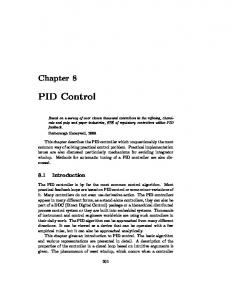
To estimate the process model parameters on-line while keeping the controller remains intact is discussed in this section. First, the apparent time delay θ is calculated from the process control signal u(t) and its derivative signal u(t). ˙ The signal u(t) from the state model (4) is generated from the combined effect of the relay and the controller. Three different parts in u(t) activate the limit cycle output y(t) during the online relay test. The composite control signal is rewritten as u(t) = ±h + Kco y(t − θ) + Kio

(7)

(14)

The time derivative of u(t) is

u(t) u1(t)

h

u (t )

(8)

x(t0 ) = (I + eAT )−1 A−1 (2eA(T +t0 −θ) − eAT − I)bu(t) (9)

(15)

It is evident from Fig. 2 and (17) that if the relay output

Time

where, I is an identity matrix of the order of A and the initial value of the state

0

t0

t1

t2

θ -h

T

Similarly, for the time range t1 < t ≤ t2 , (10)

Since the limit cycle is symmetrical, it follows x(t2 + t0 ) = −x(t0 ) and so the necessary conditions for a limit cycle with a hysteresis relay can be written y(t0 ) = cx(t0 ) = ε; y(t ˙ 0 ) = cx(t ˙ 0) > 0

y(t − θ) dt

u(t) ˙ = Kco y(t ˙ − θ) + Kio y(t − θ)

A symmetrical relay with amplitude ±h and hysteresis ±ε is used in the proposed method. In the state model (4), it is assumed that the three inputs to the process contribute the limit cycle output. The state equations for the symmetrical waveform for various time ranges over a output period T are easily obtained as follows. For the time range t0 ≤ t ≤ t1

x(t) = eA(t−t1 ) x(t1 ) − A−1 (eA(t−t1 ) − I)bu(t)

Zt 0

0

x(t) = eA(t−t0 ) x(t0 ) + A−1 (eA(t−t0 ) − I)bu(t)

MODEL PARAMETERS

(11)

Finally, the output expression (5) can be obtained by substituting the constants of (6) in (8) for the time range t0 ≤ t ≤ t1

Fig. 2.

Half limit cycle output, Control signals and its derivative

u1 (t) switches from one position to other, the control signal u(t) shall respond to the same position switching. While in case with u(t), ˙ the expression (17) gives |u(t ˙ 0 )| > 0 at t = t0 and u(t ˙ 1 ) = 0 at t = t1 . Thus, u(t) ˙ will not respond the u1 (t) switching till it has continued its monotonic movement to zero

crossing. This apparent time delay observes in Fig. 2 which is estimated as θ = t1 − t0 from the measurements of t0 and t1 . Now, the remaining parameters of the process model are obtained by using the limit cycle expressions (12) and (13). By taking the first derivative of y(t) with respect to time t and further simplifying using (12) at t = t0 , y(t0 ) = ε, the expression is obtained as y(t ˙ 0) =

kh − ε k 2 Kco h θ/T1 + (e − 1) T1 T1

(16)

Similarly, another simplified expression is obtained from (13) and its derivative y(t) ˙ at time t2 = T and y(t2 ) = 0. y(T ˙ )=−

T −t1 kh Kco − −T −k 2 h(− +Kio )(1−2e T1 +e T1 ) (17) T1 T1

From the tuning test, the half period time, the derivative of y(t) at two instants t = t0 and t2 , T , y(t ˙ 0 ) and y(T ˙ ) are measured respectively. Now, after solving the two simultaneous expressions (16) and (17) using measured values, the unknown parameters k and T1 are calculated. IV. PID

TUNING METHOD

The design method in [11] can be extended to tune PID controller to improve the output performance with special emphasis on minimizing control efforts. Let us take a PID controller C(s) to denote the subsequently tuned controller which is described by C(s) = Kc (1 +

1 + Td s) Ti s

(18)

where, Kc , Ti and Td are the controller parameters. It is straightforward to obtain PID tuning formulae based on ITAE performance index which was evaluated for PI controller tuning [11]. The explicit equations derive in terms of process model parameters are Ti /T1 =

1 + 2θn + θn2 1 + θn

(19)

Ti kKc = 1 + θn

(20)

Td = Ti /4

(21)

The extension to full PID configuration is straightforward by assuming an empirical relationship between Td and Ti , e.g. Td = 0.25Ti [12]. Thus, all developments to be described remain directly applicable for PID controllers. Using (19-21), the new PID parameters are calculated after the on-line relay test. Now, to test the optimal control loop performance, the input variations of the control signal are obtained to compare the results with other cited methods. The input variations is defined as a measure of the “smoothness” of a signal to evaluate the manipulated input usage [13]. The total variation (TV) is computed as TVu =

∞ X i=1

|ui+1 − ui |

(22)

TABLE I I DENTIFIED MODELS AND CONTROLLER SETTINGS FOR SIMULATION EXAMPLES

Process G1

Initial Co (s) 0.51 + 0.28/s

G2

0.8 + 0.2/s

Model 0.9999e−1.477s 1.757s+1 1.0e−1.792s 1.671s+1

New C(s) 0.65 + 0.31/s + 0.34s 0.62 + 0.29/s + 0.33s

To overcome the effect of load disturbance during autotuning test, the controller has to remain in the loop. In the proposed auto-tuning method, the controller is always in action even at the time of relay test. Therefore, the closed loop transfer function of the process with respect to the load disturbance can be written as y(s) G(s) = (23) d(s) 1 + G(s)(Nr + C(s)) where, Nr is the relay gain. Because of the integral action present in the controller, a symmetrical steady state limit cycle is observed even in presence of load disturbance. It is to be noted that the basic relay auto-tuner leads to an asymmetric limit cycle output that produces erroneous results in estimatation of the limit cycle parameters. V. S IMULATION

STUDIES

To demonstrate the simplicity and effectiveness of the proposed scheme, typical processes used in the relevant literature have been considered. The initial setting of PI controller and the new parameters settings after on-line tuning are shown in Table I. To overcome the possible failure, the width of the relay hysteresis is set to twice that of the standard deviation of the noise and the relay height is set such that it produces a limit cycle with acceptable amplitude level. For ease in presentation of simulation results, the symmetrical relay with height h = ±1 and hysteresis width ε = ±0.1 is considered for the following processes. G1 (s) =

e−s (s + 1)2

(24)

G2 (s) =

−s + 1 (s + 1)3

(25)

For the stable process G1 (s), Tan et al. [1] have proposed a PID controller C(s) = 0.621(1 + 1.111/s + 0.23s) using their direct, multiple point on-line tuning method. Using the proposed on-line tuning method, the identified transfer function model and the PID controller setting are obtained as shown in Table I. The closed loop responses, compared with [1] are shown in Fig. 3 and 4. It is evident that the proposed design method is not only simple, but also gives a much improved performance. The proposed scheme gives total variation TVu = 1.02, while TVu = 4.2 for the Tan et al’s method. The above values show that the proposed control method has smooth input change. Next, the nonminimum phase process G2 (s) identified by the proposed on-line tuning test with a FOPDT model and corresponding estimated PID gains are shown in the second

5

5 4

4

3 3 y(t)

y(t)

2 2

1 1 0 a b c

0

−1 0

10

20

30

40 Time (s)

50

60

70

a b c

−1 −2 0

80

Fig. 3. (a) Setpoint input, (b) responses by the proposed method and (c) by Tan et al’s method.

10

20

30

40 Time (s)

50

60

70

80

Fig. 5. (a) Setpoint input, (b) responses by the proposed method and (c) by Zhuang et al’s method.

6

8

5 6 4 4 u(t)

u(t)

3 2

2

1 0 0 a b c

−1 −2 0

10

20

30

40 Time (s)

50

60

70

a b c

−2

80

Fig. 4. (a) Setpoint input, (b) control signals by the proposed method and (c) by Tan et al’s method.

row of Table I. Using the basic relay autotuning method and the ISTE tuning proposed by Zhuang et al. [9], the PID parameters Kc = 1.35, Ki = 0.601 and Kd = 0.919 are calculated. The closed loop responses are shown in Fig. 5 and 6. The proposed method shows smooth response without any overshoot and its total variations of u(t) is 4.23 while in the case with [9], TVu = 15.10. It is observed that the method by [9] have large variation in control input of the process there by resulting in more overshoot and large settling time in compared to the proposed method. VI. C ONCLUSIONS In this paper, a simple but robust structure is proposed to tune PI/PID controller without disturbing closed-loop control. Differently from those relay based autotuning methods, it allows the tuning of controller in the presence of static load disturbance without resetting the relay. Exact analytical expressions are derived for estimating process models in terms of few measurements on half limit cycle output. The advantageous feature of such control has been illustrated by simulation results. R EFERENCES [1] K. K. Tan, T. H. Lee, X. Jiang, Robust on-line relay automatic tuning of PID control system, ISA Trans. 39 (2) (2000) 219–232.

−4 0

10

20

30

40 Time (s)

50

60

70

80

Fig. 6. (a) Setpoint input, (b) control signals by the proposed method and (c) by Zhuang et al’s method.

[2] T. S. Schei, A method for closed loop automatic tuning of PID controllers, Automatica 28 (3) (1992) 587–591. [3] W. K. Ho, Y. Honga, A. Hanssonb, H. Hjalmarssonc, J. W. Denga, Relay auto-tuning of PID controllers using iterative feedback tuning, Automatica 39 (2003) 149–157. [4] S. Majhi, On-line PI control of stable processes, J. Proc. Contr. 15 (2005) 859–867. [5] T.-S. Tsay, On-line computing of PI/lead compensators for industry processes with gain and phase specifications, Comp. Chem. Eng. 33 (2009) 14681474. ˚ om, T. H¨agglund, PID Controllers: Theory, Design and Tuning. [6] K. J. Astr¨ Instrument, Society of America, Research Triangle Park, 1995. [7] A. O’Dwyer, Handbook of PI and PID Controller Tuning Rules, Imperial College Press, 2003. [8] A. A. Rovira, P. W. Murrill, C. J. Smith, Tuning controllers for setpoint changes, Instr. Control Syst. 42 (1969) 6769. [9] M. Zhuang, D. P. Atherton, Automatic tuning of optimum PID controllers, IEE Proc.-Contr. Theory Appl. 140 (1993) 216–224. [10] P. Klan, R. Gorez, Balanced tuning of pi controllers, European J. Contr. 6 (2000) 541 – 550. [11] P. Klan, R. Gorez, Simple analytic rules for balanced tuning of PI controllers, Proceedings 2nd IFAC Conference on Control System Design (2004) 47–52. [12] W. Tang, Q. G. Wang, X. Lu, Z. P. Zhang, Why Ti=4Td for PID Controller Tuning, in: 9th International Conference on Control, Automation, Robotics and Vision, Singapore, 2006. [13] S. Skogestad, Simple analytic rules for model reduction and pid controller tuning, J. Proc. Contr. 13 (2003) 291309.