On-Line IPA Gradient Estimators in Stochastic Continuous Fluid Models Benjamin Melamed ∗ Dept. of MSIS Rutgers University Piscataway, NJ 08854
[email protected]
Yorai Wardi ∗ School of Electrical Engineering Georgia Institute of Technology Atlanta, GA 30332
[email protected]
Christos G. Panayiotou † Dept. of Manufacturing Engineering Boston University Boston, MA 02215
[email protected]
Christos G. Cassandras † Dept. of Manufacturing Engineering Boston University Boston, MA 02215
[email protected]
Submitted to Journal of Optimization Theory and Applications July 2001
Abstract This paper applies Infinitesimal Perturbation Analysis (IPA) to loss-related and workloadrelated metrics in a class of Stochastic Flow Models (SFM). It derives closed-form formulas for gradient estimators of these metrics with respect to various parameters of interest, such as buffer size, service rate and inflow rate. The IPA estimators derived are simple and fast to compute, and are further shown to be unbiased and nonparametric in the sense that they can be computed directly from observed data without any knowledge of the underlying probability law. These properties hold the promise of utilizing IPA gradient estimates as an ingredient of on-line management and control of telecommunications networks. While this paper considers single-node SFMs, the analysis method developed is amenable to extensions to networks of SFM nodes with more general topologies. Key words and phrases. Stochastic Fluid Models (SFM), Infinitesimal Perturbation Analysis (IPA), network management and control.
∗
Supported in part by the National Science Foundation under grant DMI-0085659 and by DARPA under contract F30602-00-2-0556. † Supported in part by the National Science Foundation under grants EEC-95-27422 and ACI-98-73339, by AFOSR under contract F49620-98-1-0387, by the Air Force Research Laboratory under contract F30602-99-C-0057 and by EPRI/ARO under contract WO8333-03.
1
1
Introduction
Monte Carlo simulation methods for performance evaluation of telecommunications networks have traditionally relied on queueing models. The bulk of events in such models are comprised of packet/cell arrivals and service completions followed by routing at network nodes. However, the sheer numbers of such events in simulations of high-speed telecommunications networks present serious computational problems, since simulation runs can require copious computing times and considerable storage even over relatively short time horizons. To illustrate, an ATM connection transporting 53-byte cells at the 622 megabits-per-second rate may require processing of over a million events per simulated second. In ATM networks comprised of multiple connections, the event rate is proportionately higher. To ameliorate this problem, a Stochastic Fluid Model (SFM) class has been proposed for modeling workload flow in lieu of traditional packet-based queueing models. The SFM paradigm adopts a fluid-flow worldview rather than the transaction-flow worldview of traditional queueing models. Accordingly, the description of the SFM construct substitutes inflow-rate and service-rate processes for the familiar arrival and service processes in traditional queueing models. First introduced in [1] and further developed in [7] for the analysis of multiplexed data streams, SFMs have gained acceptance as a tool for simulating high-speed networks [6, 8, 10, 9, 16, 15]. SFM-based modeling of high-speed packet/cell-based networks has been justified by analogy to fluid flows that consist of a multitude of molecules (packets/cells), but where the effect of an individual molecule on the totality of the fluid stream (traffic process) is virtually infinitesimal. We point out, however, that SFMs are not suitable for all types of network topologies, as was shown in [9, 16]. Recently, the SFM paradigm has been investigated from the standpoint of Infinitesimal Perturbation Analysis (IPA) — a sample path technique for obtaining gradients of performance metrics with respect to parameters of interest. It was conjectured in [15], based on preliminary work, that IPA would yield unbiased gradient estimators for a large class of networks in SFM setting (unlike the traditional queueing network setting). It was further conjectured that such estimators would be nonparametric in the sense that they would be computable directly from an observed sample path, without knowledge of the underlying probability law. This would render them applicable not only in simulation setting, but also in real-life on-line setting, where a node “observes” the traffic process flowing though it and computes appropriate gradient estimates. These, in turn, may be used for practical network management and control. Prior work reported in [4] has developed unbiased nonparametric IPA estimators for the loss volume and buffer workload, as functions of buffer size. This paper follows up on these results and extends them in the following directions. 1. This paper considers more general functional forms for the inflow rate and service rate processes. Previously assumed piecewise-constant in [4], this paper admits general piecewise-differentiable (and possibly discontinuous) sample paths of these processes. While the piecewise constancy assumption is essential in simulation applications, it may be hard to justify in some real-life systems (for instance, data inflow from a bursty source may not be best characterized as piecewise constant). Furthermore, permitting the service rate to have a general form can facilitate extensions of the analysis to SFM networks (see [13]). 2. This paper considers the same performance functions treated in [4] (loss volume and buffer workload). However, while [4] treated only the buffer size parameter, here we purvey IPA 2
gradient estimators with respect to additional parameters, namely, service rate and inflow rate. 3. The unbiasedness analysis in [4] was based on a finite-difference derivation of IPA derivatives — an intuitive but complicated and highly specialized technique. In contrast, the analysis here is based on general principles developed in [13], which give rise to much shorter proofs and further holds out the promise of network extensions. The rest of the paper is organized as follows. Section 2 describes the SFM construct and associated performance functions of interest. Sections 3 – 5 develop nonparametric unbiased IPA gradient estimators for loss volume and buffer workload, as functions of buffer size (Section 3), service rate (Section 4), and inflow rate (Section 5). Section 6 concludes the paper, and the appendix contains all proofs of unbiasedness.
2
Stochastic Fluid Models c
x
α δ
γ
β
Figure 1: Basic SFM Figure 1 depicts a schematic of an SFM variant, henceforth to be referred to as a basic SFM. Such a system has been considered in [13] in the context of sensitivity analysis and under general assumptions on the underlying stochastic processes. The basic SFM is a “fluidized queue”, consisting of a singleserver preceded by a fluid buffer (finite or infinite) with a single-class fluid source. Six stochastic processes over a common probability space, (Ω, F, P ), are associated with a basic SFM, as follows. 1. {α(t)}: the input flow rate (inflow) process into the SFM. 2. {β(t)}: the service rate process, namely, the maximal fluid discharge rate from the server. 3. {c(t)}: the buffer capacity (buffer size) process. 4. {x(t)}: the buffer workload (occupancy) process, namely, the fluid volume in the buffer. 5. {δ(t)}: the fluid discharge rate (outflow) process from the server. 6. {γ(t)}: the loss rate (overflow) process due to a full buffer. The first three processes, {α(t)}, {β(t)} and {c(t)}, characterize the behavior of an SFM, and are referred to as defining processes (cf [14, 15, 13]). The other three processes, {x(t)}, {δ(t)}, and {γ(t)}, are determined by the defining processes, and are referred to as derived processes. All processes evolve in a given time horizon [0, T ], for some fixed T > 0.
3
In this paper, the inflow process, {α(t)}, and the service rate process, {β(t)}, are assumed to be piecewise continuously-differentiable with probability 1 (w.p.1).1 The buffer capacity is assumed to be a given constant c > 0.2 The SFM under consideration can be viewed as a dynamical system whose input consists of the defining processes, its state is comprised of the workload process, and its output includes the outflow and overflow processes. The buffer workload process is defined by the one-sided differential equation, 0,
if x(t) = 0 and α(t) − β(t) ≤ 0 dx(t) = 0, if x(t) = c and α(t) − β(t) ≥ 0 dt+ α(t) − β(t), otherwise,
(2.1)
whose initial condition henceforth will be assumed to be x(0) = 0. The outflow rate process is defined by ( β(t), if x(t) > 0 (2.2) δ(t) = α(t), if x(t) = 0 and the overflow rate is defined by γ(t) =
(
α(t) − β(t) if x(t) = c 0, if x(t) < c.
(2.3)
We mention that outflow processes, {δ(t)}, are important in SFM networks [13], since the outflow from a node is part of the inflow into a downstream node. However, outflow processes will not concern us any further in this paper, since our interest lies here in single-node SFMs. We shall be concerned with two sample performance measures (random variables), the loss volume and the cumulative workload (also called work) over the interval [0, T ], defined by loss volume : LV = cumulative workload (work) : LW =
RT 0
γ(t) dt,
(2.4)
x(t) dt.
(2.5)
RT 0
Observe that the notational dependence on the sample ω is suppressed to simplify the presentation, as is the notational dependence on T on the left-hand sides. The corresponding expectations, ℓV = E[LV ] and ℓW = E[LW ], are performance measures (metrics). The related metrics, ℓV /T (average loss rate over [0, T ]) and ℓW /T (average buffer workload over [0, T ]), are of interest in applications. Suppose that the SFM under consideration depends on a real-valued parameter θ, assumed to belong to a closed and bounded interval, Θ.3 For instance, θ might be a parameter related to the buffer size, service rate or inflow rate. To indicate the parametric dependence of the defining processes on θ we will write {α(θ; t)}, {β(θ; t)} and c(θ), and in a similar vein, we will write {x(θ; t)} and {γ(θ; t)} for derived processes. Finally, this parametric dependence carries over in a natural way to the sample performance functions, namely, loss volume : LV (θ) = cumulative workload (work) : LW (θ) = 1
RT 0
RT 0
γ(θ; t) dt,
(2.6)
x(θ; t) dt,
(2.7)
By a piecewise continuously differentiable function we mean a piecewise-continuous function that is continuouslydifferentiable on each of its continuity intervals. 2 The case where the buffer capacity is a function of time can be important in the analysis of multi-flow networks [13]. 3 The vector case can be handled similarly, but we treat here the scalar-parameter case to simplify the notation.
4
and their expectations are similarly denoted by ℓV (θ) = E[LV (θ)] and ℓW (θ) = E[LW (θ)], respectively. We will be interested in estimating the derivatives of these two functions with respect to θ via IPA, and henceforth use prime notation to denote exclusively derivatives with respect to θ. Accordingly, ′ ′ we will be concerned with estimating the derivatives ℓV (θ) and ℓW (θ) via their IPA estimators — the ′ ′ sample derivatives LV (θ) and LW (θ), respectively. Comprehensive discussions of IPA derivatives and their applications can be found in [5, 2]. Here, we merely outline the main results germane to the present discussion. Let L(θ) be a sample performance ′ function of θ, and let ℓ(θ) = E[L(θ)] denote its expectation. The IPA estimator of ℓ (θ) (also called the ′ IPA derivative) is defined as the sample derivative, L (θ). An IPA derivative is said to be unbiased, ′ ′ ′ if it yields an unbiased estimator of ℓ (θ), namely, if ℓ (θ) = E[L (θ)]. The unbiasedness property is necessary for the practicality of IPA-based gradient estimation, since the sample (IPA) derivative obtained can then be used in optimization and possibly control via stochastic gradient-descent techniques. The unbiasedness property of IPA derivatives has been shown to be ensured by the following two conditions ([11], Lemma A2, p.70): ′
Condition 1. For every θ ∈ Θ, the sample derivative L (θ) exists w.p.1. Condition 2. W.p.1, the random function L(·) is Lipschitz-continuous throughout Θ, and the Lipschitz constant has a finite first moment. x c
Empty Period
Partial Period
Full Period
Partial Period
Empty Period
t
Figure 2: Empty Periods, Partial Periods, Full Periods Any time horizon [0, T ] can be partitioned into three types of periods (see Figure 2), in accordance with the state of the buffer, as follows: 1. An empty period (EP) is a maximal interval during which the buffer is empty. 2. A partial period (PP) is a supremal interval during which the buffer is neither full nor empty. 3. A full period (FP) is a maximal interval during which the buffer is full. An alternative partition of the time horizon [0, T ] into idle periods and busy periods is based on an analogy with queueing systems. In the SFM setting, an idle period is a maximal interval during which the server does not process fluid, and a busy period is a supremal interval during which the server discharges fluid from the system. Note that the former partition into empty periods, partial periods and full periods corresponds to the state of the buffer, whereas the latter partition into idle periods and busy periods corresponds to the state of the server. The former partition is more useful to the setting of SFM, in whose analysis it will play an important role below. The opposite (complement) of an empty period should not be confused with a busy period, since the buffer may be empty while processing fluid (see Eq. (2.2) under the conditions that x(t) = 0 while 0 < α(t) ≤ β(t)). We term such a period nonempty period (NP) or buffering period (BP), and define it to be a supremal interval during which the buffer is nonempty. Observe that a nonempty period is a superposition (union) of partial periods and full periods. 5
We later will assume that the inflow-rate process α(θ; t) and the service-rate process β(θ; t) are piecewise continuous in t for a given fixed θ. Therefore, we adopt the convention that empty periods and full periods are closed intervals, while partial periods and nonempty periods are open intervals, unless containing one of the end points, 0 or T . x c
Empty Period
Nonempty Period
Empty Period
Nonempty Period
Empty Period
t
Figure 3: Empty Periods, Nonempty Periods For a fixed θ ∈ Θ, the (given) horizon interval [0, T ] is partitioned into alternating empty periods and nonempty periods (buffering periods), as shown in Figure 3. Let the (increasing) sequence of nonempty (buffering) periods be denoted by {Bk : k = 1, . . . , K}, for some integer K ≥ 0 (in Figure 3, K = 2). By Eqs. (2.6) and (2.7), the sample performance functions under consideration can be represented as loss volume : LV (θ) = cumulative workload : LW (θ) = ′
PK
R
k=1 Bk γ(θ; t) dt, PK R k=1 Bk x(θ; t) dt.
(2.8) (2.9)
′
Since we are concerned with the sample derivatives LV (θ) and LW (θ), we need to identify conditions under which they exist. To this end, we define the notion of events along a sample path (not to be confused with simulation events). For a given fixed θ ∈ Θ, An exogenous event is a jump in either α(θ; t) or β(θ; t) (by “jump” we mean a discontinuity in t), while an endogenous event corresponds to the buffer becoming either full or empty. We will later assume that multiple events cannot occur simultaneously — certainly a mild and reasonable assumption. In each of the next three sections we consider the two performance functions of interest, the loss volume LV (θ) of Eq. (2.6) and the cumulative workload LW (θ) of Eq. (2.7), both over a given (fixed) ′ time horizon [0, T ]. Each section derives formulas for the corresponding IPA derivatives, LV (θ) and ′ LW (θ), with respect to three types of parameters θ, respectively: buffer size, parameters of the service rate, and parameters of the inflow rate. In all three sections, the IPA derivative will be shown to be nonparametric as well as unbiased, but all proofs of unbiasedness are collected in Appendix A.
3
IPA Derivatives with Respect to Buffer Size
In this section, the parameter θ is the buffer size, i.e., c(θ) = θ, and θ ∈ Θ for a given closed and bounded interval Θ whose left-hand point is positive. Assume that the processes {α(t)} and {β(t)} are independent of the parameter θ. Since the sample functions of α(t) and β(t) are assumed piecewise continuously-differentiable, it follows that, w.p.1, there exists a sequence of time points 0 = t0 < t1 < . . . < tN < tN +1 = T , for some integer N > 0 (all generally dependent upon the sample path ω), such that, 1. For each i = 1, . . . , N , the time point ti is either a jump (discontinuity) point of α(t) − β(t), or 6
α(ti ) − β(ti ) = 0. Note that in the latter case, one may have an interval with α(t) − β(t) = 0, in which case an arbitrary “representative” point ti is selected from that interval. 2. For each i = 0, . . . , N , α(t) − β(t) is continuously differentiable in the interval [ti , ti+1 ], and is either positive-valued, negative-valued, or zero-valued throughout that interval. Observe that in view of Eq. (2.1), a time point at which the buffer becomes full or empty is ′ generally a function of θ. Denoting such a point by t(θ), the derivative t (θ) exists as long as t(θ) is not a jump point of the difference process {α(t) − β(t)}. Note that the time points at which the buffer ceases to be full or empty are locally independent of θ, because they correspond to a change of sign in α(t) − β(t), which is independent of θ by assumption.4 Excluding the possibility of multiple ′ co-occurrence of events, the only situation precluding the existence of the sample derivatives LV (θ) ′ and LW (θ) involves a time interval throughout which the buffer is full and α(t) − β(t) = 0 (see Eq. ′ ′ (2.3)). However, in this case, the one-sided derivatives of LV (θ) and LW (θ) still exist. In order to keep the analysis simple, we will confine the discussion to the differentiable case, and assume accordingly that the above sample derivatives exist w.p.1 at any fixed θ ∈ Θ. Throughout this section, we make the following assumption. Assumption 3.1. (a) W.p.1, the function α(t) − β(t) is piecewise continuously-differentiable in the interval [0, T ]. (b) For every θ ∈ Θ, w.p.1, no multiple event occur simultaneously. ′
′
(c) For every θ ∈ Θ, the sample derivatives LV (θ) and LW (θ) exist, w.p.1. Fix θ ∈ Θ. As mentioned above, the start points of nonempty (buffering) periods are locally independent of θ, while the end points of such periods are locally differentiable functions of θ. Let us denote the nonempty periods in [0, T ] by Bk = (ξk , ηk (θ)),
k = 1, . . . , K,
for some K > 0, where ξk and ηk (θ) are, respectively, the start point and the end point of Bk . The nonempty periods can be classified according to whether or not they experienced some loss. Define the index set Φ(θ) = {k ∈ {1, . . . , K} : some loss occurs during Bk }, (3.1) and let NT (θ) = |Φ(θ)| denote cardinality of Φ(θ). For each k ∈ Φ(θ), let Mk be the number of full periods in Bk , and denote the associated full periods in increasing order by Fk,m = [uk,m (θ), vk,m ],
m = 1, . . . , Mk ,
where uk,m (θ) and vk,m denote, respectively, the start time and end time of Fk,m . in view of Assumption 3.1, the start times uk,m = uk,m (θ) of Fk,m are generally locally differentiable functions of θ. In contrast, the end times vk,m are locally independent of θ, since they correspond to jumps or changes of sign of α(t) − β(t), which is assumed independent of θ. A typical sample path is depicted in Figure 4, where K = 3, Φ(θ) = {1, 3}, M1 = 2, and M3 = 1. 4 A function f (θ) is locally independent of θ, if for any given θ ∈ Θ, there exists an open interval containing θ, where ′ ′ the derivative f (·) exists and f (·) = 0.
7
x c
BP
BP
t
BP
Figure 4: Typical Sample Path
3.1
Derivative of Loss Volume with Respect to Buffer Size
Let Assumption 3.1 be in effect, and consider the loss volume sample performance function, LV (θ), given by Eq. (2.6), as function of the buffer size. The following result was obtained in [4] for the case where α(t) and β(t) were piecewise-constant functions of t. Although the present case is more general in that the functions α(t) and β(t) are assumed to be piecewise continuously differentiable, the proof in [4] still works in our case. Nevertheless, we present the proof, since its arguments form the basis for the analysis of other parameters to be discussed in subsequent sections (see also [15]). Proposition 3.1. For every θ ∈ Θ,
′
LV (θ) = −NT (θ).
(3.2)
In words, the requisite derivative is just the negative number of nonempty periods in the time horizon [0, T ], during which some loss occurred. Proof. By Eqs. (2.8) and (2.3), we have LV (θ) =
X Z
k∈Φ(θ)
ηk (θ)
γ(θ; t) dt,
(3.3)
ξk
and by differentiating, we obtain d LV (θ) = dθ k∈Φ(θ) ′
X
Z
ηk (θ)
γ(θ; t) dt.
(3.4)
ξk
Observe that although Φ(θ) is a function of θ, it may be treated in Eq. (3.4) as constant in θ for x c
ξk
u
k,1
v
u
k,1
k,2
v
k,2
η
k
t
Figure 5: Typical Nonempty Period the purpose of differentiation, in view of the following justification. Assumption 3.1 implies that for a given fixed θ ∈ Θ, there exists w.p.1 ∆θ > 0, such that for every θ¯ ∈ (θ − ∆θ, θ + ∆θ), one has ¯ = Φ(θ). Although ∆θ generally depends on θ and ω, we are concerned here with derivatives at Φ(θ) θ along a particular sample path ω. Next, fix k ∈ Φ(θ), and let the nonempty period Bk = (ξk , ηk (θ)) contain Mk full periods Fk,m = [uk,m (θ), vk,m ], m = 1, . . . , Mk . A typical sample path is depicted in Figure 5, where Mk = 2. Define 8
the function ΛV,k (θ) =
Z
ηk (θ)
γ(θ; t) dt.
(3.5)
ξk
We now proceed to prove that ′
ΛV,k (θ) = −1,
(3.6)
hence Eq. (3.2) immediately follows, in view of Eqs. (3.3) – (3.4). To this end, note that by Eq. (2.3), ΛV,k (θ) =
Mk Z X
vk,m
[α(t) − β(t)] dt.
(3.7)
m=1 uk,m (θ)
Since the points uk,m(θ), m = 1, . . . , Mk , and the jump points of α(t) − β(t) constitute events, and since by Assumption 3.1, the co-occurrence of multiple events is excluded w.p.1, it follows that the function α(t) − β(t) is continuous w.p.1 at the points uk,m (θ). Consequently, differentiating Eq. (3.7) yields ′
ΛV,k (θ) = −
Mk X
′
[α(uk,m (θ)) − β(uk,m (θ))] uk,m (θ).
(3.8)
m=1
We now evaluate the terms in the sum above for two separate cases, using Figure 5 as a visual aid. Case 1: m = 1 in Eq. (3.8). Since the buffer is neither full nor empty in the interval (ξk , uk,1 (θ)), and since the buffer occupancy climbs in that interval from 0 to θ, Eq. (2.1) implies Z
uk,1 (θ)
[α(t) − β(t)] dt = θ,
ξk
which yields upon differentiation ′
[α(uk,1 (θ) − β(uk,1 (θ))] uk,1 (θ) = 1.
(3.9)
Case 2: m > 1 in Eq. (3.8). Since the buffer is neither full nor empty in the interval (vk,m−1 , uk,m (θ)), and since x(θ; vk,m−1 ) = x(θ; uk,m (θ)) = θ, Eq. (2.1) implies Z
uk,m (θ)
[α(t) − β(t)] dt = 0,
vk,m−1
which yields upon differentiation ′
[α(uk,m (θ)) − β(uk,m (θ))] uk,m (θ) = 0.
(3.10)
Finally, Eqs. (3.8), (3.9) and (3.10) imply Eq. (3.6), which was shown to imply the requisite result (3.2). 2 ′
It is evident from Eq. (3.2) that the IPA derivative LV (θ) is nonparametric, since its computation requires only counting those nonempty periods during which some loss occurs. To illustrate, Figure 4 has LV ′ (θ) = −2. No knowledge is required on the probability law underlying the defining processes, {α(t)} and {β(t)} nor on the details of the functional form of their sample paths, beyond Assumption 3.1. In fact, a simple counter at a network switch or interface point can perform the computation on-line, and possibly use such IPA derivative estimates in management and control. 9
3.2
Derivative of Cumulative Workload with Respect to Buffer Size
Let Assumption 3.1 be in effect, and consider the cumulative-workload (work) sample performance function, LW (θ), given by Eq. (2.7), as function of buffer size. The next result and its proof are similar to those in [4], where it was assumed that α(t) and β(t) are piecewise-constant functions. Proposition 3.2. For every θ ∈ Θ, ′
X
LW (θ) =
[ηk (θ) − uk,1 (θ)].
(3.11)
k∈Φ(θ)
In words, the contribution to the requisite derivative of each nonempty period Bk , during which some loss occured, is the length of the time interval starting at the first point in Bk at which the buffer becomes full and ending at the last point of Bk . Proof. If k ∈ / Φ(θ) then d dθ
Z
x(θ; t)dt = 0,
Bk
since the buffer size does not affect the workload process in Bk . Therefore, and in light of Eq. (2.9), it suffices to consider only nonempty periods that incur loss. Consider a fixed k ∈ Φ(θ), and let the nonempty period Bk = (ξk , ηk (θ)) contain Mk full periods Fk,m = [uk,m (θ), vk,m ], m = 1, . . . , Mk . A typical scenario is depicted in Figure 5, where Mk = 2. Next, define the function Z
ηk (θ)
x(θ; t) dt.
(3.12)
ΛW,k (θ) = ηk (θ) − uk,1 (θ),
(3.13)
ΛW,k (θ) =
ξk
It remains to prove that ′
from which Eq. (3.11) immediately follows. To this end, observe that since x(θ; t) is continuous in t, and since x(θ; ηk (θ)) = 0, differentiating Eq. (3.12) yields Z
′
ΛW,k (θ) =
ηk (θ)
′
x (θ; t) dt.
(3.14)
ξk
To evaluate this partial derivative, we consider four cases corresponding to three regions of the nonempty period Bk = (ξk , ηk (θ)) (refer to Figure 5 for a visual aid). Region 1: t ∈ (ξk , uk,1 (θ)) in Eq. (3.14). Here, the buffer is neither empty nor full, so in view of Eq. (2.1), x(θ; t) =
Z
t
[α(τ ) − β(τ )] dτ.
ξk ′
Since x(θ, t) is independent of θ in the equation above, it follows that x (θ; t) = 0 in this region. ′
Region 2: t ∈ (uk,m (θ), vk,m ), m = 1 . . . , Mk in Eq. (3.14). Here, x(θ, t) = θ, hence x (θ; t) = 1.
10
Region 3: t ∈ (vk,m , uk,m+1 (θ)), m = 1, . . . , Mk − 1 or t ∈ (vk,Mk , ηk (θ)) in Eq. (3.14). Here, the buffer is neither empty nor full in the interval (vk,m , t), and x(θ; vk,m ) = θ. Therefore, in view of Eq. (2.1), Z t
x(θ; t) = θ +
[α(τ ) − β(τ )] dτ,
vk,m
m = 1, . . . , Mk ,
′
so upon differentiation, we obtain x (θ; t) = 1. ′
′
In summary, x (θ; t) = 0 for t ∈ (ξk , u1 (θ)) (Region 1), and x (θ; t) = 1 for t ∈ (uk,1 (θ), ηk (θ)) (Regions 2-3). Combining these facts with Eq. (3.14) yields Eq. (3.13), which implies the requisite Eq. (3.11). 2 ′
It is evident from Eq. (3.11) that the IPA derivative LW (θ) is nonparametric, since its computation only requires the identification of time points uk,1 (θ) at which the buffer becomes full, and the time points ηk (θ) at which the buffer becomes empty.
3.3
Unbiasedness of IPA Derivatives with Respect to Buffer Size
¯ be the number of time-points t ∈ [0, T ] at which the difference function Let the random variable K α(t) − β(t) either changes sign (including becoming 0), or has a discontinuity. The unbiasedness of the IPA derivatives of loss volume and cumulative workload with respect to buffer size is established in the following proposition. Proposition 3.3. Under Assumption 3.1, the following hold: ¯ < ∞, then the IPA derivative L′ (θ) is unbiased. 1. If E[K] V ′ 2. The IPA derivative LW (θ) is unbiased. Proof. See Appendix A.
2
We mention that the proof of Proposition 3.3 is based on a general analysis technique developed in [13], and is considerably simpler and of wider scope than the proof of the analogous result in [4].
4
IPA Derivatives with Respect to Service Rate
In this section, the parameter θ is a parameter of the service rate process {β(θ; t)}, and θ ∈ Θ for a given closed and bounded interval Θ. Assume that the inflow process, {α(t)} and the buffer size, c, are independent of θ. Assume further that for all θ ∈ Θ and for all t ∈ [0, T ], ′ dβ (θ; t) = β (θ; t) = 1. dθ
(4.1)
Such functional dependence corresponds to uniform variations in the service rate. We mention in passing that the forthcoming analysis can be extended to more general functional dependencies, as will become evident in the next section, but here we consider the specific form of Eq. (4.1) in order to explain the main ideas via a simple yet useful example. For a given fixed θ, the service rate process, {β(θ; t)}, is assumed to be piecewise continuouslydifferentiable in t, with a finite number of jump points in the interval [0, T ]. From Eq. (4.1), these 11
jump points are independent of θ, though they depend on the sample path. By the assumed piecewise continuous differentiability of β(θ; t), for every θ ∈ Θ there exists w.p.1 an integer N and an increasing sequence of time points 0 = t0 < t1 (θ) < · · · < tN (θ) < tN +1 = T , such that, 1. For each i = 1, . . . , N , the time point ti (θ) is either a jump point of α(t) − β(θ; t), or a point where α(t) − β(θ; t) = 0 (if it is a jump point, then it is independent of θ). 2. For each i = 0, . . . , N , α(t) − β(θ; t) is continuously differentiable in the interval (ti (θ), ti+1 (θ)), and is either positive-valued, negative-valued, or zero-valued throughout that interval. Throughout this section, we make the following assumption. Assumption 4.1. For every θ ∈ Θ: (a) W.p.1, the function α(t) − β(θ; t) is piecewise continuously-differentiable in the interval [0, T ]. (b) W.p.1, no multiple events may occur simultaneously. ′
′
(c) The sample derivatives LV (θ) and LW (θ) exist, w.p.1. Next, fix θ ∈ Θ, and let the nonempty periods in [0, T ] be denoted in increasing order by Bk = (ξk (θ), ηk (θ)),
k = 1, . . . , K,
for some K > 0. We note that each start point, ξk (θ), and each end point, ηk (θ), are locally functions of θ, and by Assumption 4.1, these functions are differentiable at a given point θ. Let Φ(θ) of Eq. (3.1) be the index set of lossy nonempty periods, and for every k ∈ Φ(θ), partition the nonempty period Bk into alternating partial periods and full periods (see Section 2). Finally, denote the full periods of Bk in increasing order by Fk,m = [uk,m (θ), vk,m (θ)], m = 1, . . . , Mk , and note that both each start time uk,m(θ) and each end time vk,m (θ) are locally continuously-differentiable functions of θ. See Figure 5 for a typical sample path, where Mk = 2.
4.1
Derivative of Loss Volume with Respect to a Service Rate Parameter
Let Assumption 4.1 be in effect, and consider the loss volume sample performance function, LV (θ), given by Eq. (2.6), as function of a service rate parameter, subject to Eq. (4.1). Proposition 4.1. For every θ ∈ Θ, ′
LV (θ) = −
X
[vk,Mk (θ) − ξk (θ)].
(4.2)
k∈Φ(θ)
In words, the contribution to the requisite derivative of each nonempty period Bk , during which some loss occured, is the length of the time interval from the start of Bk until the last time point in Bk at which the buffer is full. Proof. If k ∈ / Φ(θ) then no loss occurs during the nonempty period Bk , and d dθ
Z
γ(θ; t)dt = 0. Bk
12
Therefore, and in view of Eq. (2.8), it suffices to consider only k ∈ Φ(θ). Consider a fixed k ∈ Φ(θ), and let the nonempty period Bk = (ξk (θ), ηk (θ)) contain Mk full periods Fk,m = [uk,m (θ), vk,m (θ)], m = 1, . . . , Mk . A typical scenario is depicted in Figure 5, where Mk = 2. Next, define the function ΛV,k (θ) =
Z
ηk (θ)
γ(θ; t) dt.
(4.3)
ξk (θ)
It remains to prove that ′
ΛV,k (θ) = −[vk,Mk (θ) − ξk (θ)],
(4.4)
which clearly implies Eq. (4.2). To this end, decompose Eq. (4.3) with the aid of Eq. (2.3) as ΛV,k (θ) =
Mk Z X
vk,m (θ)
γ(θ; t) dt
(4.5)
m=1 uk,m (θ)
(see Figure 5 for a visual aid, where Mk = 2), and differentiate Eq. (4.5) to obtain ′
ΛV,k (θ) =
Z Mk X d
m=1
dθ
vk,m (θ)
γ(θ; t) dt.
(4.6)
uk,m (θ)
We next analyze the derivative terms on the right-hand side of Eq. (4.6). Recalling that for all t ∈ [uk,m (θ), vk,m (θ)], one has γ(θ; t) = α(t) − β(θ; t), and that dβ(θ;t) = 1 by Eq. (4.1), we have dθ dγ(θ;t) = −1. Consequently, we can write dθ d dθ
vk,m (θ)
Z
γ(θ; t) dt =
uk,m (θ) ′
− [vk,m (θ) − uk,m(θ)] + [α(vk,m (θ)− ) − β(θ; vk,m (θ)− )] vk,m (θ) ′
− [α(uk,m (θ)+ ) − β(θ; uk,m (θ)+ )] uk,m (θ).
(4.7)
But since the buffer becomes full at every time point uk,m (θ), it follows that each of them is an event, as are the jump points of α(t) − β(θ; t), and Assumption 4.1 mandates the continuity of α(t) − β(θ; t) at each points um (θ) by excluding the simultaneous occurrence of multiple events. Therefore, α(uk,m (θ)+ ) − β(θ; uk,m (θ)+ ) = α(uk,m (θ)) − β(θ; uk,m (θ)), and consequently, d dθ
Z
vk,m (θ)
γ(θ; t) dt =
uk,m (θ) ′
− [vk,m (θ) − uk,m(θ)] + [α(vk,m (θ)− ) − β(θ; vm (θ)− )] vk,m (θ) ′
− [α(uk,m (θ)) − β(θ; uk,m (θ))] uk,m (θ),
m = 1, . . . , Mk .
(4.8)
We now evaluate the terms in the sum above as two separate cases, using Figure 5 as a visual aid. Case 1: m = 1 in Eq. (4.8). As shown in Figure 5, x(θ; ·) ascends from 0 to c in the interval [ξk (θ), uk,1 (θ)]. Hence, by Eq. (2.1), Z
uk,1 (θ)
[α(t) − β(θ; t)] dt = c.
ξk (θ)
13
(4.9)
Recalling that
dβ(θ;t) dt
= 1 by Eq. (4.1), differentiating Eq. (4.9) yields ′
′
−[uk,1 (θ) − ξk (θ)] + [α(uk,1 (θ)) − β(θ; uk,1 (θ))] uk,1 (θ) − [α(ξk (θ)+ ) − β(θ; ξk (θ)+ )] ξk (θ) = 0. (4.10) We now show that the last term on the left-hand side of (4.10) vanishes. To this end, observe that ξk (θ) is a point at which the buffer ceases to be empty under one of two scenarios: either α(t) − β(θ; t) jumps at ξk (θ), or α(t) − β(θ; t) is continuous and becomes positive at ξk (θ). In the first scenario, ′ it was shown that jump times in α(t) − β(θ; t) are independent of θ, hence ξk (θ) = 0. In the second scenario, we must have α(ξk (θ)+ )− β(θ; ξk (θ)+ ) = α(ξk (θ))− β(θ; ξk (θ)) = 0. Thus, in either scenario, ′ [α(ξk (θ)+ ) − β(θ; ξk (θ)+ )] ξk (θ) = 0. Consequently, Eq. (4.10) reduces to ′
−[uk,1 (θ) − ξk (θ)] + [α(uk,1 (θ)) − β(θ; uk,1 (θ))] uk,1 (θ) = 0.
(4.11)
Substituting Eq. (4.11) into Eq. (4.8) for m = 1 now yields d dθ
Z
vk,1 (θ)
γ(θ; t) dt =
uk,1 (θ) ′
−[vk,1 (θ) − uk,1 (θ)] + [α(vk,1 (θ)− ) − β(θ; vk,1 (θ)− )] vk,1 (θ) − [uk,1 (θ) − ξk (θ)].
(4.12)
Case 2: m > 1 in Eq. (4.8). As shown in Figure 5 (for Mk = 2), for every m = 2, . . . , Mk , Z
uk,m (θ)
[α(t) − β(θ; t)] dt = 0,
(4.13)
vk,m−1 (θ)
which yields on differentiation, ′
− [uk,m (θ) − vk,m−1 (θ)] + [α(uk,m (θ)) − β(θ; uk,m (θ))] uk,m (θ) ′
− [α(vk,m−1 (θ)+ ) − β(θ; vk,m−1 (θ)+ )] vk,m−1 (θ) = 0.
(4.14)
We next show that for all m = 2, . . . , M + 1, ′
′
[α(vk,m−1 (θ)+ ) − β(θ; vk,m−1 (θ)+ )] vk,m−1 (θ) = [α(vk,m−1 (θ)− ) − β(θ; vk,m−1 (θ)− )] vk,m−1 (θ) = 0. (4.15) To this end, observe that vk,m−1 (θ) is a point at which the buffer ceases to be full under one of two scenarios: either α(t) − β(θ; t) jumps at t = vk,m−1 (θ), or α(t) − β(θ; t) is continuous at t = vk,m−1 (θ) and switches sign there from non-negative to non-positive. In the first scenario, it was shown that ′ jump times in α(t) − β(θ; t) are independent of θ, hence vk,m−1 (θ) = 0. In the second scenario, α(vk,m−1 (θ)+ ) − β(θ; vk,m−1 (θ)+ ) = α(vk,m−1 (θ)− ) − β(θ; vk,m−1 (θ)− ) = α(vk,m−1 (θ)) − β(θ; vk,m−1 (θ)) = 0. Thus, in either scenario, Eq. (4.15) is satisfied. Consequently, Eq. (4.14) reduces to ′
−[uk,m (θ) − vk,m−1 (θ)] + [α(uk,m (θ)) − β(θ; uk,m (θ))] uk,m (θ) = 0.
14
(4.16)
Substituting Eq. (4.16) into Eq. (4.8) for m = 2, . . . , Mk now yields d dθ
Z
vk,m (θ)
uk,m (θ)
γ(θ; t) dt = −[vk,m(θ) − uk,m (θ)] ′
+ [α(vk,m (θ)− ) − β(θ; vk,m (θ)− )] vk,m (θ) − [uk,m (θ) − vk,m−1 (θ)].
(4.17)
Next, apply Eq. (4.15) with m = 2 to Eq. (4.12), and with m = 3, . . . , Mk + 1 to Eq. (4.17), and observe that the middle terms vanish on the right-hand sides of these equations. Consequently, Eq. (4.12) reduces to Z d vk,1 (θ) γ(θ; t) dt = −[vk,1 (θ) − ξk (θ)], (4.18) dθ uk,1 (θ) and Eq. (4.17) reduces to d dθ
Z
vk,m (θ)
uk,m (θ)
γ(θ; t) dt = −[vk,m (θ) − vk,m−1 (θ)],
m = 2, . . . , Mk .
(4.19)
Finally, in view of Eq. (4.6), summing Eqs. (4.18) and (4.19) results in Eq. (4.4), which implies the requisite Eq. (4.2). 2 ′
It is evident from Eq. (4.2) that the IPA derivative LV (θ) is nonparametric, since its computation requires only the detection of boundaries of empty periods and full periods.
4.2
Derivative of Cumulative Workload with Respect to a Service Rate Parameter
Let Assumption 4.1 be in effect, and consider the cumulative workload (work) sample performance function, LW (θ), given by Eq. (2.7), as function of a service rate parameter, subject to Eq. (4.1). Let us define vk,0 (θ) = ξk (θ) and uk,Mk +1 (θ) = ηk (θ), k = 1, . . . , K. Proposition 4.2. For every θ ∈ Θ, ′
LW (θ) = −
K MX k +1 1X [uk,m (θ) − vk,m−1 (θ)]2 . 2 k=1 m=1
(4.20)
Proof. Consider a given fixed k ∈ {1, . . . , K}, and let the nonempty period Bk = (ξk (θ), ηk (θ)) contain Mk full periods Fk,m = [uk,m (θ), vk,m (θ)], m = 1, . . . , Mk . Note that the case Mk = 0, namely k∈ / Φ(θ), whose corresponding term in (4.20) is [ηk (θ) − ξk (θ)]2 , is also included. A typical scenario with Mk = 2 is shown in Figure 5. Next, define the function ΛW,k (θ) =
Z
ηk (θ)
x(θ; t) dt.
(4.21)
ξk (θ)
We will prove that ′
ΛW,k (θ) = −
Mk +1 1 X [uk,m (θ) − vk,m−1 (θ)]2 , 2 m=1
15
(4.22)
from which Eq. (4.20) immediately follows. Note that by Eq. (4.21), the continuity of x(θ; t) in t, and the fact that x(θ; ξk (θ)) = x(θ; ηk (θ)) = 0, ′
ΛW,k (θ) =
ηk (θ)
Z
′
x (θ; t) dt.
(4.23)
ξk (θ) ′
It remains, therefore, to derive the appropriate expressions for the derivative x (θ; t) and substitute them in (4.23). First, observe that during any full period Fk,m = [uk,m (θ), vk,m (θ)], m = 1, . . . , Mk , one has the equality x(θ; t) = c, for all t ∈ Fk,m , hence ′
x (θ; t) = 0,
t ∈ Fk,m .
(4.24)
Next, consider t in any partial period (vk,m−1 (θ), uk,m (θ)), m = 1, . . . , Mk + 1. By Eq. (2.1), x(θ; t) = x(θ; vk,m−1 (θ)) +
Z
t
[α(τ ) − β(θ, τ )] dτ.
(4.25)
vk,m−1 (θ)
Noting that x(θ; vk,m−1 (θ)) =
(
0, if m = 1 c, if m = 2, . . . , Mk + 1
(see Figure 5), we conclude that d x(θ; vk,m−1 (θ)) = 0, dθ
m = 1, . . . , Mk + 1.
Consequently, taking derivative with respect to θ in (4.25) we obtain, ′
x (θ; t) =
Z
t
′
vk,m−1 (θ)
′
−β (θ; τ ) dτ − [α(vk,m−1 (θ)+ ) − β(θ; vk,m−1 (θ)+ )] vk,m−1 (θ).
We now argue that
′
[α(vk,m−1 (θ)+ ) − β(θ; vk,m−1 (θ)+ )] vk,m−1 (θ) = 0,
(4.26)
(4.27)
as a product of two terms, one of which must vanish. To see that, we consider two possibilities. If the point vk,m−1 (θ) is a jump (discontinuity) point of the function α(t) − β(θ; t), then it is independent of ′ θ, implying vk,m−1 (θ) = 0. Conversely, if is not a jump point, then vk,m−1 (θ) must be a point at which the buffer ceases to be empty (m = 1) or full (m > 1), so that the function α(t) − β(θ; t) changes sign there from nonpositive to non-negative (m = 1) or from non-negative to nonpositive (m > 1), and in either case, α(vk,m−1 (θ)) − β(θ; vk,m−1 (θ)) = 0. The validity of Eq. (4.27) is thus established. ′
Finally, substituting Eq. (4.27) into Eq. (4.26) yields, in view of the assumption β (θ; t) = 1, ′
x (θ; t) = −[t − vk,m−1 (θ)],
t ∈ [vk,m−1 (θ), uk,m (θ)].
Eqs. (4.23) and (4.28) now imply the requisite Eq. (4.22). ′
(4.28) 2
It is evident from Eq. (4.20) that the IPA derivative LW (θ) is nonparametric, since its computation requires only the detection of the boundaries of partial periods.
16
4.3
Unbiasedness of IPA Derivatives with Respect to a Parameter of Service Rate
The unbiasedness of the IPA derivatives of loss volume and cumulative workload with respect to a service rate parameter, subject to Eq. (4.1), is established in the following proposition. ′
′
Proposition 4.3. Under Assumption 4.1, the IPA derivatives LV (θ) and LW (θ) are unbiased. Proof. See Appendix A.
5
2
IPA Derivatives with Respect to a Parameter of Inflow Rate
In this section, the parameter θ is a parameter of the inflow rate process {α(θ; t)}, and θ ∈ Θ for a given closed and bounded interval Θ. There is a similarity to the case of the service-rate parameter ′ discussed in Section 4. For instance, if α (θ; t) = 1 for all θ ∈ Θ and t ∈ [0, T ], then similar results to Proposition 4.1 and Proposition 4.2 are in force, except for the minus sign in Eqs. (4.2) and (4.20). ′ However, the functional form α (θ; t) = 1 throughout Θ × [0, T ] is not quite realistic, since it makes little sense to perturb the inflow rate incrementally when all of the input sources are off, namely α(θ; t) = 0. A more realistic functional form of α(θ; t) was considered in [15], where ′
α (θ; t) =
(
1, if α(θ; t) > 0, 0, if α(θ; t) = 0,
(5.1)
corresponding to uniform variations in the inflow rate of an active source. Here we extend this functional dependence to a more general class of inflow rate processes {α(θ; t)}. Suppose that, for a given fixed θ ∈ Θ, the function α(θ; t) − β(t) is piecewise continuously differentiable in t, and its jump points do not depend on θ. As in the previous two subsections, we define an event to be the occurrence of either a jump in the difference process α(θ; t) − β(t), or a situation where the buffer becomes full or empty. Suppose that for every t ∈ [0, T ], the function α(θ; t) is differentiable ′ in θ, namely the derivative α (θ; t) exists throughout the set Θ × [0, T ]. An example is provided by Eq. (5.1), where a unit rate is uniformly added to an active source. We consider again the performance functions LV (θ) and LW (θ), as defined in Eqs. (2.6) and (2.7). ′ ′ Their IPA derivatives, LV (θ) and LW (θ), will be shown to be nonparametric as long as the partial ′ derivative α (θ; t) has a nonparametric form (e.g., Eq. (5.1)). Throughout this section, we make the following assumption. Assumption 5.1. (a) For every θ ∈ Θ, w.p.1, the function α(θ; t) − β(t) is piecewise continuously-differentiable in the interval [0, T ]. (b) For every θ ∈ Θ, w.p.1 no multiple events may occur simultaneously. ′
′
(c) For every θ ∈ Θ, the sample derivatives LV (θ) and LW (θ) exist, w.p.1. (d) The jump points of α(θ; t) (as function of t) do not depend on θ.
17
(e) For every t ∈ [0, T ], the function α(θ; t) is continuously differentiable in θ. There exits K < ∞ such that, w.p.1, ′ sup{|α (θ; t)| : θ ∈ Θ; t ∈ [0, T ]} ≤ K. As before, fix θ ∈ Θ, and let the nonempty periods in [0, T ] be denoted in increasing order by Bk = (ξk (θ), ηk (θ)),
k = 1, . . . , K,
for some K > 0. Let Φ(θ) of Eq. (3.1) be the index set of lossy nonempty periods, and for every k ∈ Φ(θ), partition the nonempty period Bk into alternating partial periods and full periods (see Section 2). Finally, denote the full periods of Bk in increasing order by Fk,m = [uk,m (θ), vk,m (θ)], m = 1, . . . , Mk , and define vk,0 (θ) = ξk (θ) and uk,Mk +1 (θ) = ηk (θ). A typical sample path is depicted in Figure 5, where Mk = 2.
5.1
Derivative of Loss Volume with Respect to an Inflow Rate Parameter
Let Assumption 5.1 be in effect, and consider the loss volume sample performance function, LV (θ), given by Eq. (2.6), as function of an inflow parameter. Proposition 5.1. For every θ ∈ Θ, X Z
′
LV (θ) =
vk,Mk (θ)
′
α (θ; t) dt.
(5.2)
k∈Φ(θ) ξk (θ)
Proof. If k ∈ / Φ(θ) then certainly d dθ
Z
γ(θ; t)dt = 0, Bk
and hence it suffices to consider only k ∈ Φ(θ). Fix k ∈ Φ(θ), and let the nonempty period Bk = (ξk (θ), ηk (θ)) contain Mk full periods, Fk,m = [uk,m (θ), vk,m (θ)], m = 1, . . . , Mk . Define the function Z
ΛV,k (θ) =
ηk (θ)
γ(θ; t) dt.
(5.3)
ξk (θ)
We next prove that ′
ΛV,k (θ) =
Z
vk,Mk (θ)
′
α (θ; t) dt,
(5.4)
ξk (θ)
from which Eq. (5.2) readily follows. To this end, observe that Eqs. (2.3) and (5.3) imply ΛV,k (θ) =
Mk Z X
vk,m (θ)
γ(θ; t) dt,
(5.5)
m=1 uk,m (θ)
and differentiation of Eq. (5.5) yields ′
ΛV,k (θ) =
Z Mk X d
m=1
dθ
18
vk,m (θ)
uk,m (θ)
γ(θ; t) dt.
(5.6)
We now analyze the derivative terms on the right-hand side of Eq. (5.6). Since γ(θ; t) = α(θ; t) − β(t) for all t ∈ (uk,m (θ), vk,m (θ)), one has d dθ
Z
vk,m (θ)
γ(θ; t) dt =
uk,m (θ)
vk,m (θ)
Z
′
α (θ; t) dt
uk,m (θ) ′
′
+ [α(θ; vk,m (θ)− ) − β(vk,m (θ)− )] vk,m (θ) − [α(θ; uk,m (θ)+ ) − β(uk,m (θ)+ )] uk,m (θ). (5.7) Since the buffer becomes full at the time point uk,m (θ) and simultaneous multiple events are excluded, α(θ; t) − β(t) must be continuous at the point t = uk,m(θ). Using these facts in Eq. (5.7) yields d dθ
Z
vk,m (θ)
γ(θ; t) dt =
uk,m (θ)
Z
vk,m (θ)
′
α (θ; t) dt
uk,m (θ) ′
′
+ [α(θ; vk,m (θ)− ) − β(vk,m (θ − )] vk,m (θ) − [α(θ; uk,m (θ)) − β(uk,m (θ))] uk,m (θ).
(5.8)
We now evaluate the terms in the equation above as two separate cases. Case 1: m = 1 in Eq. (5.8). In this case, x(θ; t) ascends from 0 to c in the interval [ξk (θ), uk,1 (θ)], hence by Eq. (2.1), Z
uk,1 (θ)
[α(θ; t) − β(t)] dt = c.
(5.9)
ξk (θ)
Differentiating Eq. (5.9) and recalling (Assumption 5.1 (b)) that α(θ; t)− β(t) is continuous at uk,1 (θ), we obtain Z
uk,1 (θ)
ξk (θ)
′
′
′
α (θ; t) dt + [α(θ; uk,1 (θ)) − β(uk,1 (θ))] uk,1 (θ) − [α(θ; ξk (θ)+ ) − β(ξk (θ)+ )] ξk (θ) = 0. (5.10)
We next argue that the last term on the left-hand side of (5.10) vanishes. There are two possible scenarios. If α(θ; t) − β(t) is continuous at ξ(θ), then α(θ; ξk (θ)) − β(ξk (θ)) = 0. Conversely, if it is ′ not continuous at ξk (θ), then ξk (θ) = 0 by virtue of part (d) of Assumption 5.1. In either scenario, the last term on the left-hand side of Eq. (5.10) is the product of two terms, one of which always vanishes. Consequently, Eq. (5.10) reduces to Z
uk,1 (θ)
ξk (θ)
′
′
α (θ; t) dt + [α(θ; uk,1 (θ)) − β(uk,1 (θ))] uk,1 (θ) = 0.
(5.11)
Substituting Eq. (5.11) into Eq. (5.8) for m = 1, we obtain d dθ
Z
vk,1 (θ)
uk,1 (θ)
γ(θ; t) dt =
Z
vk,1 (θ) uk,1 (θ)
′
′
α (θ; t) dt + [α(θ; vk,1 (θ)− ) − β(vk,1 (θ)− )] vk,1 (θ) +
Z
uk,1 (θ)
′
α (θ; t) dt.
ξk (θ)
(5.12)
Case 2: m > 1 in Eq. (5.8). Since x(θ; vk,m−1 (θ)) = x(θ; uk,m(θ)) = c and in view of Eq. (2.1), one has Z uk,m (θ)
[α(θ; t) − β(t)] dt = 0,
vk,m−1 (θ)
which yields upon differentiation and in view of the continuity of α(θ; t) − β(t) at uk,m (θ)), Z
uk,m (θ)
vk,m−1 (θ)
′
′
α (θ; t) dt + [α(θ; uk,m (θ)) − β(uk,m (θ))] uk,m (θ) ′
− [α(θ; vk,m−1 (θ)+ ) − β(vk,m−1 (θ)+ )] vk,m−1 (θ) = 0. 19
(5.13)
The last term on the left-hand side of Eq. (5.13) vanishes, since it is the product of two terms one of which always vanishes. Therefore, Eq. (5.13) reduces to Z
uk,m (θ)
vk,m−1 (θ)
′
′
α (θ; t) dt + [α(θ; uk,m (θ)) − β(uk,m (θ))] uk,m (θ) = 0.
(5.14)
Substituting Eq. (5.14) into Eq. (5.8), we obtain d dθ
Z
vk,m (θ)
γ(θ; t) dt =
uk,m (θ)
Z
vk,m (θ)
uk,m (θ)
′
−
′
−
α (θ; t) dt + [α(θ; vk,m (θ) ) − β(vk,m (θ) )] vk,m (θ) +
Z
uk,m (θ)
′
α (θ; t) dt. (5.15)
vk,m−1 (θ)
Next, for every m = 1, . . . , Mk , vk,m (θ) is a time point at which the buffer ceases to be full, and consequently, ′ [α(θ; vk,m (θ)− ) − β(vk,m (θ)− )] vk,m (θ) = 0, (5.16) since the left-hand side in Eq. (5.16) is a product of two terms, one of which always vanishes. Thus, applying Eq. (5.16) with m = 1 to (5.12) yields d dθ
Z
vk,1 (θ)
γ(θ; t) dt =
Z
vk,1 (θ)
′
α (θ; t) dt,
(5.17)
ξk (θ)
uk,1 (θ)
while applying Eq. (5.16) with m = 2, . . . , Mk to Eq. (5.15) yields d dθ
Z
vk,m (θ)
γ(θ; t) dt =
Z
uk,m (θ)
′
α (θ; t) dt.
(5.18)
vk,m−1 (θ)
uk,m (θ)
From Eqs. (5.17), (5.6) and (5.18) it readily follows that Eq. (5.4) holds, which implies the requisite Eq. (5.2). 2
5.2
Derivative of Cumulative Work with Respect to an Inflow Rate Parameter
Let Assumption 5.1 be in effect, and consider the cumulative-workload sample performance function, LW (θ), given by Eq. (2.7), as function of an inflow parameter, θ. Recall the definitions vk,0 (θ) = ξk (θ) and uk,Mk +1 (θ) = ηk (θ). Proposition 5.2. For every θ ∈ Θ, ′
LW (θ) =
K MX k +1 Z X
k=1 m=1
uk,m (θ)
Z
t
′
α (θ; τ ) dτ dt.
(5.19)
vk,m−1 (θ) vk,m−1 (θ)
Proof. Fix k ∈ {1, . . . , K}, and let the nonempty period Bk = (ξk (θ), ηk (θ)) contain Mk full periods Fk,m = [uk,m (θ), vk,m (θ)], m = 1, . . . , Mk , in increasing order. Define the function ΛW,k (θ) =
Z
ηk (θ)
ξk (θ)
20
x(θ; t) dt.
(5.20)
It suffices to prove that MX k +1 Z uk,m (θ)
′
ΛW,k (θ) =
Z
t
′
α (θ; τ ) dτ dt,
(5.21)
vk,m−1 (θ) vk,m−1 (θ)
m=1
from which Eq. (5.19) readily follows. To this end, differentiate Eq. (5.20), and noting that x(θ; ·) is continuous in t and x(θ; ξk (θ)) = x(θ; ηk (θ)) = 0, one has ′
ΛW,k (θ) =
Z
ηk (θ)
′
x (θ; t) dt.
(5.22)
ξk (θ) ′
It remains to derive the appropriate expressions for the derivative x (θ; t) and substitute them into Eq. (5.22). First, observe that x(θ; t) = c throughout any full period Fk,m = [uk,m (θ), vk,m (θ)], m = 1, . . . , Mk , and hence ′ x (θ; t) = 0, t ∈ Fk,m . (5.23) Next, Eq. (2.1) implies that for any partial period, (vk,m−1 (θ), uk,m (θ)), m = 1, . . . , Mk + 1, x(θ; t) = x(θ; vk,m−1 (θ)) +
Z
t
[α(θ; τ ) − β(τ )] dτ,
vk,m−1 (θ)
Since x(θ; vk,m−1 (θ)) =
(
t ∈ (vk,m−1 (θ), uk,m (θ)).
(5.24)
0, if m = 1 c, if m = 2, . . . , Mk + 1,
it follows that
d x(θ; vk,m−1 (θ)) = 0, m = 1, . . . , Mk + 1, dθ and taking derivative with respect to θ in (5.24) results in ′
x (θ; t) =
Z
t
′
vk,m−1 (θ)
′
α (θ; τ ) dτ − [α(θ; vk,m−1 (θ)+ ) − β(vk,m−1 (θ)+ )] vk,m−1 (θ).
(5.25)
We now show that in Eq. (5.25), ′
[α(θ; vk,m−1 (θ)+ ) − β(vk,m−1 (θ)+ )] vk,m−1 (θ) = 0,
(5.26)
arguing that this expression is a product of two terms, one of which must vanish. To see this, we consider two possible scenarios: either vk,m−1 (θ) is a jump (discontinuity) point or it is a continuity point of α(θ; t)−β(t). If vk,m−1 (θ) is a jump point, then it is independent of θ by part (d) of Assumption ′ 5.1, hence vk,m−1 (θ) = 0. Conversely, if it is a continuity point, then vk,m−1 (θ) must be a point at which the buffer either ceases to be empty (m = 1) or ceases to be full (m > 1). In the former case (m = 1), α(θ; t) − β(t) changes sign there from nonpositive to non-negative, and in the latter case (m > 1), it changes sign there from non-negative to nonpositive. Either way, α(θ; vk,m−1 (θ)) − β(vk,m−1 (θ)) = 0, and we conclude that Eq. (5.26) is valid. Finally, from Eqs. (5.25) and (5.26), we obtain ′
x (θ; t) =
Z
t
′
α (θ; τ ) dτ, vk,m−1 (θ)
t ∈ [vk,m−1 (θ), uk,m (θ)],
and the requisite Eq. (5.19) follows from Eqs. (5.27), (5.22) and (5.21). 21
(5.27) 2
5.3
Unbiasedness of IPA Derivatives with Respect to a Parameter of Inflow Rate
The unbiasedness of the IPA derivatives of loss volume and cumulative workload with respect to an inflow parameter is established in the following proposition. ′
′
Proposition 5.3. Under Assumption 5.1, the IPA derivatives LV (θ) and LW (θ) are unbiased. Proof. See Appendix A.
6
2
Conclusion
The discontinuous nature of sample performance functions, inherent in traditional queueing models, has long hampered the application of IPA to gradient estimation by giving rise to biased estimators. In contrast, the continuous nature of their fluid model counterparts has been demonstrated in this paper to give rise to corresponding IPA estimators which are unbiased, nonparametric and computable in real time. In addition to these favorable theoretical properties, loss-related and workload-related performance functions hold the promise of broad applications in the context of management and control of high-speed telecommunications networks. In an earlier work [12] we conjectured that IPA would give rise to unbiased derivative estimators in networks from a large class of stochastic fluid models. This paper provides an initial step in the exploration of the scope of IPA application to fluid-flow systems. It defined an elemental single-node building block model, called basic SFM, and considered two performance functions of relevance to communications applications: loss volume, and buffer workload. It then derived their IPA derivatives with respect to various parameters, including buffer size, service rate and inflow rate. The IPA derivatives obtained were shown to be nonparametric and unbiased, and surprisingly simple and fast to compute. The next step in this research program is to extend the results to SFM networks and to multiple workload flows. The main challenge concerns the modeling of routing and multiplexing, in view of the fact that the SFM setting lacks an inherent concept of individual packets. We believe, however, that such modeling is possible, as is the derivation of nonparametric IPA estimators in a general setting of SFM networks.
22
References [1] D. Anick, D. Mitra, and M.M. Sondhi, “Stochastic Theory of a Data-Handling System with Multiple Sources”, The Bell System Technical Journal, Vol. 61, 1871–1894, 1982. [2] C.G. Cassandras, Discrete Event Systems: Modeling and Performance Analysis, Aksen Associates, Irwin, Boston, MA, 1993. [3] C.G. Cassandras, G. Sun, and C.G. Panayiotou, “Stochastic Fluid Models for Control and Optimization of Systems with Quality of Service Requirements”, submitted to the 2001 IEEE Conference on Decision and Control. [4] C.G. Cassandras, Y. Wardi, B. Melamed, G. Sun and C.G. Panayiotou, “Perturbation Analysis for On-Line Control and Optimization of Stochastic Fluid Models”, submitted, 2001. [5] Y.C. Ho and X.R. Cao, Perturbation Analysis of Discrete Event Dynamic Systems, Kluwer Academic Publishers, Boston, MA, 1991. [6] G. Kesidis, A. Singh, D. Cheung, and W.W. Kwok, “Feasibility of Fluid-Driven Simulation for ATM Network”, in Proc. IEEE Globecom, Vol. 3, 2013-2017, November 1996. [7] H. Kobayashi and Q. Ren, “A Mathematical Theory for Transient Analysis of Communications Networks”, IEICE Transactions on Communications, Vol. E75-B, 1266–1276, 1992. [8] K. Kumaran and D. Mitra, “Performance and Fluid Simulations of a Novel Shared Buffer Management System”, in Proc. IEEE INFOCOM, March 1998. [9] B. Liu, Y. Guo, J. Kurose, D. Towsley, and W.B. Gong, “Fluid Simulation of Large Scale Networks: Issues and Tradeoffs”, in Proc. Intl. Conf. on Parallel and Distributed Processing Techniques and Applications, Las Vegas, Nevada, June 1999. [10] N. Miyoshi, “Sensitivity Estimation of the Cell-Delay in the Leaky Bucket Traffic Filter with Stationary Gradual Input”, in Proc. Intl. Workshop on Discrete Event Systems, WoDES’98, 190-195, Cagliari, Italy, August 26-28, 1998. [11] R.Y. Rubinstein and A. Shapiro, Discrete Event Systems: Sensitivity Analysis and Stochastic Optimization by the Score Function Method, John Wiley and Sons, New York, NY, 1993. [12] Y. Wardi and B. Melamed, “IPA Gradient Estimation for the Loss Volume in Continuous Flow Models”, in Proc. of the Hong Kong International Workshop on New Directions of Control and Manufacturing, 30–33, Hong Kong, November 1994. [13] Y. Wardi and B. Melamed, “Variational Bounds and Sensitivity Analysis of Traffic Processes in Continuous Flow Models”, J. of Discrete Event Dynamic Systems, Vol. 11, pp. 249-282, 2001. [14] Y. Wardi and B. Melamed, “Continuous Flow Models: Modeling, Simulation and Continuity Properties”, in Proc. 38th IEEE Conf. On Decision and Control, 34–39, Phoenix, Arizona, December 7-10, 1999.
23
[15] Y. Wardi and B. Melamed, “Loss Volume in Continuous Flow Models: Fast Simulation and Sensitivity Analysis via IPA”, in Proc. 8-th IEEE Mediterranean Conference on Control and Automation (MED 2000), Patras, Greece, July 17-19, 2000. [16] A. Yan and W.B. Gong, “Fluid Simulation for High-speed Networks with Flow-Based Routing”, IEEE Trans. on Information Theory, Vol. 45, 1588–1599, 1999.
24
Appendix A
Proofs of Unbiasedness of IPA Estimators
This appendix contains proofs for the unbiasedness of the IPA estimators, annunciated in Propositions 3.3, 3.4 and 3.5. These proofs rely on a common framework for general SFM networks, developed in [13] and to be reviewed briefly below. To set the stage, let {z(θ; t)} denote a defining process that depends on θ, and let {y(θ; t)} denote a generic derived process. To illustrate, if θ is a parameter of the service time process, then one has z(θ; t) = β(θ; t), and y(θ; t) might denote realizations of the derived processes, {x(θ; t)} or {γ(θ; t)}. Suppose that only one of the defining processes is a function of θ, while the two other defining processes are independent of θ. We consider a finite variation in θ, i.e., a perturbation from a given value of θ to another value, θ + ∆θ. This perturbation results in a functional variation in the θ-dependent defining process, while the two other defining processes remain unperturbed. For a given fixed θ ∈ Θ, a realization z(θ; t) of the defining process and the corresponding realizations of each of the other two defining processes, together determine the realization y(θ; t) of a derived process (all realizations correspond to a common sample point, ω ∈ Ω). For a given ω, consider a perturbation of θ in a realization of a defining process from z(θ; t) to z(θ+∆θ; t) (we assume, of course, that θ+∆θ ∈ Θ). This perturbation in the defining process determines perturbations in both derived processes, denoted generically by y(θ + ∆θ; t). Finally, let the difference processes be denoted by ∆z(t) = z(θ + ∆θ; t) − z(θ; t), and ∆y(t) = y(θ + ∆θ; t) − y(θ; t). We endow all realizations of the defining and derived processes under consideration with functional norms as follows: α(θ; t), β(θ; t) and γ(θ; t) are endowed with the L1 norm, while x(θ; t) and c(θ; t) = c(θ) are endowed with the L∞ norm (recall that c(θ; t) = c(θ) is independent of t, but is viewed here as R a constant function of time). Recall that the L1 norm of a function u : [0, T ] → R is ||u||1 = 0T |u(t)| dt, and the L∞ norm of a piecewise continuous function u : [0, T ] → R is ||u||∞ = max{|u(t)| : t ∈ [0, T ]}. The symbol || · || denotes a generic norm in either L1 or L∞ . We will be concerned with Lipschitz-type inequalities of the form ||∆y(t)|| ≤ K ||∆z(t)||,
(A.1)
for some finite K > 0. We point out that since the difference processes are random, it follows that K is a random variable; however, K is independent of z(t) or ∆z(t). In other words, Eq. (A.1) is satisfied for all z(t) and ∆z(t), and effectively indicates the Lipschitz continuity of a mapping from a space of defining processes to a space of derived processes. Such Lipschitz continuity has been established in [13], where the following two results were obtained. Consider first variations (perturbations) in α(θ; t). Proposition A.1 (cf [13], Proposition 3.1). The following inequalities hold: (a) ||∆x(t)||∞ ≤ ||∆α(t)||1 , (b) ||∆γ(t)||1 ≤ ||∆α(t)||1 .
2
Consider next variations in the service rate process, {β(θ; t)}. Proposition A.2 (cf [13], Proposition 3.2). The following inequalities hold: (a) ||∆x(t)||∞ ≤ ||∆β(t)||1 , (b) ||∆γ(t)||1 ≤ 2||∆β(t)||1 . 25
2
Finally, consider perturbations in the buffer size process, {c(θ; t)}. Since in this paper {c(θ; t)} depends only on θ but not on t, we shall use the notation ∆c = c(θ + ∆θ) − c(θ) for perturbations in buffer size. Let further K(θ) and K(θ + ∆θ) denote the number of nonempty periods contained in the interval [0, T ], when the buffer size is c(θ) and c(θ + ∆θ), respectively ([13] used the notation KN and KP ). Proposition A.3 (cf [13], Proposition 3.3). Letting K = max{K(θ), K(θ + ∆θ)}, the following inequalities hold: (a) ||∆x||∞ ≤ |∆c|, R 2 (b) | 0T ∆γ(τ )dτ | ≤ K |∆c|. Observe that part (b) does not quite yield a Lipschitz constant, since the left-hand side of the inequality is not a functional norm, and the quantity K on the right-hand side depends on both θ and θ + ∆θ.
Finally, recall the following two conditions, which are jointly sufficient for the unbiasedness of an ′ IPA derivative L (θ) ([11], Lemma A2, p.70). ′
Condition A.1 For every θ ∈ Θ, the sample derivative L (θ) exists, w.p.1.
2
Condition A.2 W.p.1, the random function L(·) is Lipschitz continuous throughout Θ, and the Lipschitz constant has a finite first moment. 2 With the aid of Condition A.1 and Condition A.2, we are now in a position to prove the unbiasedness results reported in this paper for the random functions LV (θ) and LW (θ), respectively defined by Eq. (2.6) and (2.7). Proof of Proposition 3.3. Condition A.1 is satisfied for the random functions LV (θ) and LW (θ) by part (c) of Assumption 3.1, so it only remains to establish Condition A.2 for these functions. ¯ denote the number of times that the difference function α(t) − β(t) either changes sign or Let K jumps in [0, T ]. Clearly, the number of nonempty periods contained in [0, T ] is bounded from above ¯ + 1, regardless of the buffer size. Thus, K ¯ does not depend on θ nor on θ + ∆θ. Therefore, and by K by part (b) of Proposition A.3, we have the inequality |
Z
T
¯ + 1) |∆c|. ∆γ(τ ) dτ | ≤ (K
(A.2)
0
Note that since c(θ) = θ, one has ∆c = ∆θ.
(A.3)
Consider first the sample performance function LV (θ) = | LV (θ + ∆θ) − LV (θ)| = |
Z
RT 0
γ(θ; t) dt, and observe that
T
∆γ(τ ) dτ |.
(A.4)
0
From Eqs. (A.2) - (A.4) we conclude that ¯ + 1) |∆θ|, |LV (θ + ∆θ) − LV (θ)| ≤ (K ¯ has a finite first namely, that the function LV (θ) is Lipschitz continuous. If the Lipschitz constant K ′ moment, then Condition A.2 is satisfied for LV (θ), and the IPA derivative LV (θ) is unbiased. This concludes the proof of the first part of Proposition 3.3. 26
Consider next the sample performance function LW (θ) =
RT 0
x(θ; t)dt. Noting the inequality
|LW (θ + ∆θ) − LW (θ)| ≤ T ||∆x(t)||∞ , it follows from part (a) of Proposition A.3 and from Eq. (A.3) that |LW (θ + ∆θ) − LW (θ)| ≤ T |∆θ|, which establishes that the function LW (θ) has a Lipschitz constant T . This shows that Condition A.2 is satisfied, therefore concluding the proof of the second part of Proposition 3.3. 2 Proof of Proposition 4.3. Condition A.1 is satisfied for the random variables LV (θ) and LW (θ) by part (c) of Assumption 4.1, so it only remains to establish Condition A.2 for these random variables. Consider first the sample performance function LV (θ). By Eq. (2.6), |LV (θ + ∆θ) − LV (θ)| ≤ ||∆γ(t)||1 ,
(A.5)
and from part (b) of Proposition A.2, ||∆γ(t)||1 ≤ 2 ||∆β||1 .
(A.6)
′
Noting that ||∆β||1 = T |∆θ| by the assumption β (θ; t) = 1, we conclude in view of Eqs. (A.5) and (A.6), that |LV (θ + ∆θ) − LV (θ)| ≤ 2 T |∆θ|. This establishes that LV (θ) has a Lipschitz constant 2 T , thereby establishing Condition A.2, and completing its proof of unbiasedness. Consider next the sample performance function LW (θ). By (2.7) we have the inequality |LW (θ + ∆θ) − LW (θ)| ≤ T ||∆x||∞ , which together with part (a) of Proposition A.2 and the equality ||∆β||1 = T |∆θ| imply the inequality |LW (θ + ∆θ) − LW (θ)| ≤ T 2 |∆θ|. This establishes that LW (θ) has a Lipschitz constant T 2 , thereby establishing Condition A.2, and completing its proof of unbiasedness. 2 Proof of Proposition 5.3. Condition A.1 is satisfied for the random variables LV (θ) and LW (θ) by part (c) of Assumption 5.1, so it only remains to establish Condition A.2 for these sample performance functions. By Eqs. (2.6) and (2.7) we have the respective inequalities |LV (θ + ∆θ) − LV (θ)| ≤ ||∆γ(t)||1 , |LW (θ + ∆θ) − LW (θ)| ≤ T ||∆x(t)||∞ .
(A.7) (A.8)
Furthermore, from Proposition A.1 we have the respective inequalities ||∆γ(t)||1 ≤ ||∆α(t)||1
(A.9)
||∆x(t)||∞ ≤ ||∆α(t)||1 .
(A.10)
27
Next, part (e) of Assumption 5.1 implies that there exists K < ∞, such that for all θ ∈ Θ and θ + ∆θ ∈ Θ, ||∆α(t)||1 ≤ K T |∆θ|. (A.11) Consequently, Eqs. (A.7) – (A.11) yield the inequalities |LV (θ + ∆θ) − LV (θ)| ≤ K T |∆θ|, |LW (θ + ∆θ) − LW (θ)| ≤ K T 2 |∆θ|. This establishes that LV (θ) has a Lipschitz constant K T , and LW (θ) has a Lipschitz constant K T 2 , thereby establishing Condition A.2 for both and completing their proof of their unbiasedness. 2
28