Assistance for Computer Aided Machine Control. Staffan Ekvall ... (HMMs) and Support Vector Machines (SVMs) for state ..... http://www.ascension-tech.com.
On-line Task Recognition and Real-Time Adaptive Assistance for Computer Aided Machine Control Staffan Ekvall, Daniel Aarno and Danica Kragi´c Centre for Autonomous Systems Computational Vision and Active Perception Laboratory Royal Institute of Technology (KTH) SE-100 44 Stockholm SWEDEN Phone: +46-8-7906798, Fax: +46-8-7230302 Email: {ekvall, bishop, danik}@nada.kth.se Submission for short paper Abstract Dividing the task that the operator is executing into several subtasks is one of the key research areas in teleoperative and humanmachine collaborative settings. Hence, segmentation and recognition of operator generated motions are commonly facilitated to provide appropriate assistance during task execution. This assistance is usually provided in a virtual fixture framework where the level of compliance can be altered online thus improving the performance both in terms of execution time and overall precision. However, the fixtures are typically inflexible, resulting in a degraded performance in cases of unexpected obstacles or incorrect fixture models. In this paper, we deal with the problem of on-line task tracking and propose the use of adaptive virtual fixtures that can cope with the above problems. The operator may remain in each of these subtasks as long as necessary and switch freely between them. Hence, rather than executing a predefined plan, the operator has the ability to avoid unforeseen obstacles and deviate from the model. In our system, the probability that the user is following a certain trajectory (subtask) is estimated and used to automatically adjusts the compliance. Thus, an on-line decision of how to fixture the movement is provided. Index Terms Virtual fixtures, Human-Machine Collaborative Systems, Hidden Markov Models, Support Vector Machines, Ergonomics
1
On-line Task Recognition and Real-Time Adaptive Assistance for Computer Aided Machine Control I. I NTRODUCTION N the area of Human Machine Collaborative Systems (HMCSs) and teleoperation, task segmentation and recognition are two important research problems. We show how a flexible design framework can be obtained by borrowing ideas from the area of Programming by Demonstration to build a system where a HMCS can be trained in a fast and easy way. In our system, a high-level task is segmented into subtasks where each of the subtasks has a virtual fixture obtained from 3D training data. Virtual fixtures are commonly defined as a taskdependent aid for teleoperative purposes, [1] and are used to constrain the user’s or the manipulator’s motion in undesired directions while allowing or aiding motion along the desired directions. In our work, a virtual fixture is a physical constraint that forces a robot to move along desired paths. A state sequence analyzer learns what subtasks are more probable to follow each other. This is then used by an on-line state estimator which estimates the probability of the user being in a particular state. A specific virtual fixture, corresponding to the most probable state can then be applied. In [2], the concept of Cobots as special purpose humanmachine collaborative manipulation systems used in the car industry has been presented. Although frequently used, the Cobots are specially designed for a single task and when the assembly task changes, they have to be reprogrammed. We use a combination of K-means clustering, Hidden Markov Models (HMMs) and Support Vector Machines (SVMs) for state generation, state sequence analysis and associated probability estimation. In our system, task segmentation is performed offline and used by an on-line state estimator that applies a virtual fixture with a fixturing factor determined by the probability of being in a certain state. The use of the HMM/SVM approach is motivated by the good generalization over similar tasks. The system presented in this paper considers a humanmachine collaborative or a teleoperated setting. The system consists of an off-line task learning and an on-line task execution step. An overview of the system is shown in Fig. 1. The system is fully autonomous and is able to i) decompose a demonstrated task into states, ii) compute a virtual fixture for each state and iii) aid the user with task execution by applying the correct virtual fixture at all times. A summary of methods and applications related to virtual fixtures is presented in Section II. In Section III and Section IV the theoretical methods and system implementation are presented. Experimental results are presented in Section V and Section VI concludes the paper.
I
II. R ELATED W ORK Approaches similar to ours have been considered in HMCS settings. In [3], a HMCS system is presented where virtual
Teach task
Execute task User
Fig. 1.
Record time-position tuples
Aquire time-position tuple
Find number of states (lines)
Compute input velocity
Quantize recorded samples to each state
Compute SVM probabilities
Compute a virtual fixture for each state
Compute HMM probabilities
Train one SVM for each state
Compute guidance from HMM probability
Train a HMM for the complete task using the SVMs for probability estimation
Apply virtual fixture from most probable state
Overview of the system used for task training and task execution.
fixtures facilitate tracking of a sine curve in two dimensions and a HMM framework is used to estimate whether the user is doing nothing, following or not following the curve. Based on this estimate, the virtual fixture is automatically switched on or off, enabling the user to avoid local obstacles. In [4], different ways of setting the compliance level are demonstrated, depending on how well the user is following the fixture. Three different compliance behaviors were evaluated: toggle, fade and hold. The results show that the fade behavior, which linearly decreases the compliance with the distance from the fixture, achieves best results when using automatic task detection. In our work, the compliance is adjusted through a fixturing factor presented in the next section. Instead of using the distance to the fixture, the probability that the user is in a certain state is used as a basis for setting the compliance. This approach was not evaluated by the above and is one of the contributions of our work. In many applications, the fixtures are generated from a predefined model of the task. These approaches work well as long as the trajectory to be followed in the real world is exactly as described by the model. In robotic applications, the system must be able to deal with model errors and there is a requirement to perform the same type of tasks in terms of sequencing but the length (type) of each subtask may vary. Therefore, an adaptive approach in which the trajectory is decomposed into straight lines is evaluated in this work. The system constantly estimates which state the user is currently in and aids the execution. To estimate the state, it is necessary to decompose the task into several subtasks, recognize the subtasks on-line and handle deviations from the learned task in a flexible
2
manner. For this purpose, HMMs have been commonly used to model and detect state changes corresponding to different predefined subtasks, [3], [5]. However, in most cases only one- or two-dimensional input have been considered. In our system, the subtasks are automatically detected given the assumption of motions along straight lines in 3D. Hence, a hybrid HMM/SVM automata is constructed for on-line state probability estimation. III. T HEORETICAL BACKGROUND In a collaborative system, it is important to detect the current state, i.e. user’s intention, in order to correctly guide the user. Virtual fixtures can be used to assist the user in controlling a teleoperated manipulator by constraining the motion of the manipulator through definition of virtual walls and forbidden regions or through definition of a desired directions and trajectories of motions, [6]. Another example of virtual fixtures is to directly constrain the user motion in undesired directions while allowing motion along desired directions using a haptic interface, [1]. The approach adopted in this work defines a desired direction d ∈ R3 , kdk = 1 or the span of the task, [6]–[8]. The user’s input, which may be force, position or velocity measurements, is transformed to a desired velocity vuser . The user’s desired velocity is then divided into components parallel and perpendicular to the desired direction and scaled by a fixturing factor k as shown by (1). The fixturing factor determines the compliance of the system. A high value (' 1) of k means that the fixture is hard, i.e. only motion in the direction of the fixture is allowed (low compliance). A value of k = 0.5 is in our notation equivalent to no fixture at all and supporting isotropic motion (high compliance). The output velocity v of the robot is then obtained by scaling vˆ to match the input speed as shown in (2). vˆ = projd (vuser ) · k + perpd (vuser ) · (1 − k) vˆ · kvuser k v= kˆvk
(1) (2)
A. Probability Estimators for HMM Hidden Markov Models integrate a simple and efficient temporal model and statistical modeling tools for stationary signals into a mathematical framework, [9]. A HMM, denoted by λ = (A, B, π), is defined by three elements over a collection of N states and M discrete observation symbols: • A = {ai j } is the state transition probability matrix • B = {bi (ok )} is the observation probability matrix • π = {πi } is the initial state probability vector One of the problems with HMMs is the choice of the probability distribution for estimating the observation probability matrix B. With continuous input, a parametric distribution is often assumed because of issues related to the BaumWelch method on data sets where M � N [10]. Using a parametric distribution to model the observation, similarities may decrease the performance of the HMM since the real distribution is hidden and the assumption of a parametric distribution is a strong hypothesis on the model [5]. Using
probability estimators avoids this problem. These estimators compute the observation symbol probability instead of using a look-up matrix or parametric model, [11]. Another advantage with probability estimators is that they allow to use continuous input instead of discrete observation symbols for the HMM. Successful use of probability estimators using multi layer perceptrons (MLP) and Support Vector Machines (SVM) are reported in [11], [12]. In this work, SVMs are used to estimate the observation probabilities P(x|state i). Support Vector Machines (SVM) have been used extensively for pattern classification in a number of research areas [13], [14] and have several appealing properties such as fast training, accurate classification and good generalization [15]. SVMs are binary classifiers that separate two classes by an optimal separation hyperplane which is found by minimizing the expected classification error. SVMs work with linear separation surfaces [15] and estimate a function f : χ → {±1} that classifies the input x ∈ χ to one of the two classes ±1 based on input-output training data. If we consider a class of hyperplanes w · x + b = 0, w ∈ RN , b ∈ R with the corresponding decision function f (x) = sgn(w · x + b). It was shown in [15] that the hyperplane decision function can be written as: ! m
f (x) = sgn
∑ yi · αi (x · x) + b
(3)
i=1
which implies that the solution vector w has an expansion in terms of a subset of the training samples. The subset is formed by the training samples with a non-zero Lagrange multiplier, αi . The samples with a non-zero Lagrange multiplier are known as the support vectors and are computed by solving a quadratic programming problem, [15]. IV. T RAJECTORY A NALYSIS This section describes the implementation of the virtual fixture learning system. The virtual fixtures are generated automatically from a number of demonstrated tasks. The overall task is decomposed into several subtasks, each with its own virtual fixture. According to Fig. 1, the first step is to filter the input data. Then, a line fitting step is used to estimate how many lines (states) are required to represent the demonstrated trajectory. An observation probability function learns the probabilities of observing specific 3D-vectors when tracking a specific line. Finally, a state sequence analyzer learns what lines are more probable to follow each other. In summary, the demonstrated trajectories results in a number of support vectors, a HMM and a set of virtual fixtures. The support vectors and the HMM are then used to decide when to apply a certain fixture. A. Retrieving Measurements The input data consist of a set of 3D-coordinates that may be obtained from a number of modalities, describing a (position, time) tuple {q,t}. From the input samples, movement directions are extracted. The noisy input samples are filtered using a dead-zone of radius δ around q, i.e. a minimum distance δ since the last stored sample is required so that small variations in position are not captured.
3
B. Estimating Lines in the Demonstrated Trajectories Once the task has been demonstrated, the input data is quantized in order to segment different lines. The input data consists of normalized 3D-vectors representing directions and K-means clustering [16] is used to find the lines. The position of a cluster center is equal to the direction of the corresponding line. Given a trajectory, the number of lines required to represent it has to be estimated automatically. For this purpose a search method is used that evaluates the result for different number of clusters and then chooses the quantization with the best results. Prior to clustering, two thirds of the data points are stored for validation. These are used to measure how well the current clusters represent unseen data. We estimate an optimal number of clusters that maximizes the validation score for the unseen data. The algorithm starts with a single cluster and gradually increases the number of clusters by one as long as the validation score increases. C. Estimating Observation Probabilities Using SVMs For each state detected by the clustering algorithm, a SVM is trained to distinguish it from all the others (one-vs-all). In order to provide a probability estimation for the HMM, the distance to the margin from the sample to be evaluated is computed as [5]: f j (x) = ∑ αi · yi · x · xi + b
(4)
i
where x is the sample to be evaluated, xi is the i-th training sample, yi ∈ {±1} is the class of xi and j denotes the j-th SVM. The distance measure f j (x) is then transformed to a conditional probability using a sigmoid function, g(x), [5]. The probability for a state i given a sample x can then be computed as: P(state i|x) = gi (x) · ∏(1 − g j (x)) j6=i −σ· fi (x)
where gi (x) = 1/(1 + e
(5)
)
Given the above and applying Bayes’ rule, the HMM observation probability P(x|state i) may be computed. The SVMs now serve as probability estimators for both the HMM training and state estimation. Since the standard SVMs do not cope well with outliers, a modified version of SVMs is used [17].
Fig. 2. The experimental workspace with obstacles: the white line shows the expected path of the end-effector.
states are equally probable at the start time. For training, the Baum-Welch algorithm is used until stable values are achieved. With each line, there is an associated virtual fixture defined by the direction of the line. In order to apply the correct fixture, the current state has to be estimated. The system continuously updates the state probability vector p = pi , where pi = P(xk , xk−1 ..., x1 |state i) is calculated according to (6). The state s with the highest probability ps is chosen and the virtual fixture corresponding to this state is applied with the fixturing factor k = max(0.5, ps · ξ), ξ ∈ [0, 1], where ps = maxi {pi } and ξ is the maximum value for the fixturing factor. As shown in (1), the fixturing factor describes how the virtual fixture will constrain the manipulator’s motion. In the case of a haptic input device, the fixture can also be used to provide the necessary feedback to the user and not only constraining the motion of the teleoperated device. Thus, when unsure which state the user is currently in, the user has full control. On the other hand, when all observations indicate a certain state, the fixturing factor k is set to ξ. This automatic adjustment of the fixturing factor allows the user to leave the fixture and move freely without having a special “notfollowing-fixture”-state. if plast = 0 πi · P(x|state i) Nstates pˆi = last otherwise P(x|state i) · ∑ Ai j · p j j
pi
=
pˆi /∑ pˆk
(6)
k
D. State Sequence Analysis Using Hidden Markov Models Even if a task is assumed to consist of a sequence of line motions, in an on-line execution step, the lines may have different lengths compared to the training data. When a certain line is followed, it is assumed that the corresponding line state is active. Thus, there are equally many states as there are line directions. Given that a certain state is active, some states are more likely to follow after depending on the task and, in our system, a fully connected Hidden Markov Model is used to model the task. The number of states is equal to the number of line types found in the training data. The A-matrix is initially set to have probability 0.7 to remain in the same state and a uniformly distributed probability to switch state. The π vector is set to uniformly distributed probabilities, meaning that all
V. E XPERIMENTAL E VALUATION In this section, three experiments are presented. The first experiment is a simple trajectory tracking task in a workspace with obstacles, shown in Fig. 2. The second is similar to the first one, but the workspace was changed after training, in order to test the algorithm’s automatic adjustment to similar workspaces. In the last experiment, an obstacle was placed along the path of the trajectory, forcing the operator to leave the fixture. This experiment tested the adjustment of the fixturing factor as well as the algorithm’s ability to cope with unexpected obstacles. In the experiments, a teleoperated setting was considered. The PUMA 560 robot was controlled via a magnetic tracker
4
called Nest of Birds (NOB) [18] mounted on a data-glove carried by the user. The NOB consists of a transmitter and pose measuring sensors. The glove with the sensors can be seen in the lower part of Fig. 2 - there is one sensor mounted on a thumb, index and a little finger and the fourth sensor is placed at the middle of the hand. In the experiments, only the hand sensor is used since it provides the full position and orientation estimate of the user’s hand motion. Subtask recognition is performed with a frequency of 30 Hz due to the limited sampling rate of the NOB sensor. The movements of the operator measured by the NOB sensor were used to extract a desired input velocity to the robot. After applying the virtual fixture according to (2), the desired velocity of the end effector is sent to the robot control system. Controlling the end-effector manually in this way is hard, but the experiments will show that the use of virtual fixtures makes the task easier. The system also works well with other input modalities. For instance, a force sensor mounted on the end effector has also been used to control the robot. In all experiments, a deadzone of δ = 2 cm was used. This value of δ corresponds to the approximate noise level of our input device. One of the major difficulties of the system is that the input device provides no haptic feedback. Therefore, the virtual fixture framework is used to filter out sensor noise and correct unintentional operator motions. This is done by scaling down the input velocity that is perpendicular to the desired direction of the virtual fixture as long as the commanded motions is along the general direction of the learned fixture. In all experiments, a maximum fixturing factor was ξ = 0.8. A radial basis function with σ = 2 was used as the kernel for the SVMs and the value of σ in the sigmoid transfer function (5), was empirically chosen to 0.5. A PUMA 560 robot arm was used in all experiments. A. Experiment 1: Trajectory following The first experiment was a simple trajectory following task in a narrow workspace. The user had to avoid obstacles and move along certain lines to avoid collision. At start, the operator demonstrated the task five times, the system learned from training data and four states were automatically identified. The user then performed the task again using the glove, the states were automatically recognized and the robot was controlled aided by the virtual fixtures generated from the training data. The path taken by the robot is shown in Fig. 3 (Left). For clarity, the state probabilities and fixturing factor estimated by the SVM and HMM during task execution are presented in Fig. 4 (Middle). This example clearly demonstrates the ability of the system to successfully segment and repeat the learned task, allowing a flexible state change. Initially, the end-effector is moving along the y-axis, corresponding to the direction of state 3. Because of deviations from the state direction, the SVM probability will fluctuate since its estimation is based on the distance from the decision boundary. However the HMM probability remains steady due to the estimation history. This shows the advantage of using a HMM on top of SVM for state identification. At sample 24, the user switches direction and starts raising the endeffector. The fixturing factor decreases with the probability for
state 3, simplifying the direction change. Then, the probability for state 1, corresponding to movement along the z-axis, increases. In total, the user performed 4 state transitions in the experiment. B. Experiment 2: Changed Workspace This experiment demonstrates the ability of the system to deal with a changed workspace. The same training trajectories as in the first experiment were used, but the workspace was changed after training. As it can be seen in Fig. 3 (Middle), the size of the obstacle the user has to avoid has been changed. As the task is just a variation of the trained task, the system is still able to identify the operator’s intention and correct unintentional operator motions. The trajectory generated from the on-line execution shows that the changed environment does not introduce any problem for the control algorithm since an appropriate fixturing factor is provided at each state. This clearly justifies the proposed approach compared to the work previously reported in [2]. C. Experiment 3: Unexpected Obstacle The final experiment was conducted in the same workspace as the first one. However, this time a new obstacle was placed right in the path of the learned trajectory, forcing the operator to leave the fixture. In this case, the virtual fixture is not aiding the operator, but may instead do the opposite as the operator wants to leave the fixture in order to avoid the obstacle. Hence, in this situation it is desired that the effect of the virtual fixture decreases as the operator avoids the obstacle. Once again, the same training examples as in the previous experiments were used. Fig. 3 (Right) illustrates the path taken in order to avoid the obstacle. The system always identifies the class which corresponds best with input data. Fig. 4 (Right) shows the probabilities and fixturing factor for this experiment. Initially, the task is identical to experiment 1, the user follows the fixture until the obstacle has to be avoided. The fixturing factor decreases as the user diverts from the direction of state 3, and thus the user is able to avoid the obstacle. It can be seen that the overall task has changed and that new states were introduced in terms of sequencing. The proposed system not only provides the possibility to perform the task, but can also be used to design a new task model by demonstration if this particular task has to be performed several times. VI. C ONCLUSIONS We have proposed a system based on the use of adaptive virtual fixtures. It is widely known that one of the important issues for teleoperative systems is the ability to divide the overall task into subtasks and provide the desired control in each of them. We have shown that it is possible to use a HMM/SVM hybrid state sequence analyzer on multi-dimensional data to obtain an on-line state estimate that can be used to apply a virtual fixture. Furthermore, the process is automated to allow construction of fixtures and task segmentation from demonstrations, making the system flexible and adaptive by
5
State 1 State 2 State 3 State 4
State 1 State 2 State 3 State 4
0
0
−0.1
−0.1
−0.1
−0.2
−0.2
z
0
z
z
State 1 State 2 State 3 State 4
0.5 −0.3 −0.4 0.5 −0.5
0 y
x
0.5 −0.3
0
−0.4 0.5 −0.5
0 y
−0.5 −1
−0.2
0.5 −0.3
0
View from above
0
−0.4 0.5
x
−0.5
0 y
−0.5
−1
−1
x
−0.5
−1
−1
−1
HMM SVM
1
0 10
25
50
75
100
0 10
25
50
75
100
0 10
25
50
75
100
0 0 0.8
25
50
75
100
25
50 Sample
75
100
0.5 0
Avoid Obstacle Fixturing Probability, Probability, Probability, Probability, factor state 4 state 3 state 2 state 1
Fixturing Probability, Probability, Probability, Probability, factor state 4 state 3 state 2 state 1
Fig. 3. End effector position in example workspace. The different symbols (colors) corresponds to the different states recognized by the HMM. Left) Following trajectory using virtual fixtures, Middle) Modified workspace (obstacle size), and Right) Avoid obstacle not present during training. HMM SVM
1
0 10
25
50
75
100
0 10
25
50
75
100
0 10
25
50
75
100
0 0 0.8
25
50
75
100
25
50 Sample
75
100
0.5 0
Fig. 4. Left) A training example demonstrated by the user, Middle) Estimated probabilities for the different states in experiment 1. Estimates are shown for both the SVM and HMM, the fixturing factor is also shown, and Right) Estimated probabilities for the different states in the obstacle avoidance experiment 3. Estimates are shown for both the SVM and HMM estimator.
separating the task into subtasks. Hence, model errors and unexpected obstacles are easily dealt with. In the current design, the algorithm automatically estimates the number of subtasks required to divide the training data. If instead it is possible for the user to manually select the number of states, the algorithm may be expected to perform even better. Such approach may be, for example, used in medical applications since surgical tasks are expected to be well-defined and known in advance [8]. Our current work evaluates this approach for more complex settings where motion primitives such as splines are used. This approach requires a hierarchical representation since any complex motion can locally be approximated by a line. The future work will evaluate the benefits of such a representation. R EFERENCES [1] S. Payandeh and Z. Stanisic, “On application of virtual fixtures as an aid for telemanipulation and training,” in 10th Symp. on Haptic Interfaces for Virtual Environment and Teleoperator Systems, pp. 18–23, 2002. [2] M. A. Peshkin, J. E. Colgate, W. Wannasuphoprasit, C. Moore, R. B. Gillespie, and P. Akella, “Cobot architecture,” IEEE Trans. on Robotics and Automation, vol. 17, no. 4, pp. 377–390, 2001. [3] M. Li and A. Okamura, “Recognition of Operator Motions for Real-Time Assistance Using Virtual Fixtures,” in 11th Symp. on Haptic Interfaces for Virtual Environment and Teleoperator Systems, pp. 125 – 131, 2003. [4] J. Nolin, P. Stemniski, and A. Okamura, “Activation Cues and Force Scaling Methods for Virtual Fixtures,” in Symp. on Haptic Interfaces for Virtual Env. and Teleoperator Systems, pp. 404 – 409, 2003. [5] A. Castellani, D. Botturi, M. Bicego, and P. Fiorini, “Hybrid HMM/SVM Model for the Analysis and Segmentation of Teleoperation Tasks,” in IEEE Int. Conf. on Robotics and Automation, vol. 3(2918-2923), 2004. [6] M. Li and R. Taylor, “Spatial motion constraints in medical robot using virtual fixtures generated by anatomy,” in IEEE Int. Conf. on Robotics and Automation, vol. 2, pp. 1270–1275, 2004.
[7] P. Marayong, M. Li, A. M. Okamura, and G. D. Hager, “Spatial Motion Contraints: Theory and Demonstrations for Robot Guidance Using Virtual Fixtures,” in IEEE Int. Conf. on Robotics and Automation, vol. 2, pp. 1954–1959, 2003. [8] D. Kragi´c, P. Marayong, M. Li, A. M. Okamura, and G. D. Hager, “Human-Machine Collaborative Systems for Microsurgical Applications,” in Int. Symp. on Robotics Research, 2003. [9] L. Rabiner, “A Tutorial on Hidden Markov Models and Selected Applications in Speech Recognition,” in Proc. of the IEEE, vol 77, no. 2, pp. 257–286, 1989. [10] A. Elgammal, V. Shet, Y. Yacoob, and L. S. Davis, “Learning Dynamics for Exemplar-Based Gesture Recognition,” in IEEE Conf. on Computer Vision and Pattern Recognition, vol. 1, pp. 571–578, 2003. [11] H. Bourlard and N. Morgans, “A Continuous Speech Recognition System Embedding MLP into HMM,” in Advances in Neural Information Processing Systems, vol. 2, pp. 413 – 416, 1990. [12] S. Renals, N. Morgan, H. Bourlard, M. Cohen, and H. Franco, “Connectionist probability estimators in HMM speech recognition,” IEEE Trans. on Speech and Audio Processing, vol. 2, no. 1, pp. 161–174, 1994. [13] D. Roobaert, Pedagogical Support Vector Learning: A Pure Learning Approach to Object Recognition. PhD thesis, Numerical Analysis and Computing Science, Royal Institute of Technology, Sweden, 2001. [14] K. H. P. Haesun, “Prediction of protein relative solvent accessibility with support vector machines and long-range interaction 3D local descriptor,” Proteins: Structure, Function, and Bioinformatics, pp. 557–562, 2004. [15] P.-H. Chen, C.-J. Lin, and B. Schlkopf, “A Tutorial on ν-Support Vector Machines.” http://www.csie.ntu.edu.tw/˜cjlin/ papers/nusvmtutorial.pdf. [16] J. B. MacQueen, “Some Methods for Classification and Analysis of Multivariate Observations,” in 5-th Berkeley Symp. on Mathematical Statistics and Probability, pp. 281–297, 1967. [17] C. Cortes and V. Vapnik, “Support-Vector Networks,” Machine Learning, vol. 20, no. 3, pp. 273–297, 1995. [18] “Nest of Birds.” http://www.ascension-tech.com.