On Link Reliability in Wireless Mobile Ad Hoc Networks - CiteSeerX

On Link Reliability in Wireless Mobile Ad Hoc Networks Juki Wirawan Tantra, Chuan Heng Foh

Dongyu Qiu

Centre for Multimedia and Network Technology School of Computer Engineering Nanyang Technological University Singapore

Electrical and Computer Engineering Concordia University Canada

Abstract— In mobile ad hoc networks (MANETs), packets are forwarded by a series of nodes to the desired destination. Previously, we have studied the network connectivity of MANETs. In this paper, we study the reliability of an established route between a source to a destination. The route is considered reliable only when all links in the route remain connected for packet relaying. We analyze the link reliability under the condition that the forwarding nodes are mobile. With this analysis, we derive the time period that the established route remains reliable for packet forwarding. Simulation is conducted to validate our analysis.

I. I NTRODUCTION Wireless mobile ad hoc networks (MANETs) provide solutions for rapid deployment in areas where infrastructure networks do not exist. MANETs are generally formed by a collection of wireless communications devices commonly known as nodes. The packet delivery in a MANET relies on relaying of packets from a source to a series of forwarding nodes until they reach the desired destination. Hence the reliability of these networks depends on the robustness of the link communications between forwarding nodes. In MANETs, a source must establish a route to the destination either proactively or reactively prior to actual data transmissions. In this process, a set of forwarding nodes are selected to form a route between the source and the destination depending on the routing strategy. Due to the mobility of the nodes, this route may remain reliable for a finite time period before a link breakage occurs, and link repair or route reestablishment must take place. Inevitably, a brief pause of data transmissions, or more seriously, a disconnection of a communication session between the source and the destination may appear. Hence, prediction of the robustness of a link in terms of link connectivity duration provides insight to the reliability of the communications and helps improve the routing protocol design. Our considered one-dimensional (1D) MANET is shown in Fig. 1 where nodes are constrained to one dimensional movement on, for example, a freeway or a walking path. The distance between the source node, S, to the destination node, D, is fixed i.e. the source and the destination do not move. Previously, we studied the network connectivity of such a network [1], [2]. Since the stationary property applies only to the source and the destination, forwarding nodes remain mobile. The link between two adjacent forwarding mobile nodes may break; thus, breaking an established route from

1-4244-0063-5/06/$20.00 ©2006 IEEE

1st hop

…

2nd hop S

n2

n1 Fig. 1.

d

last hop (h–1)–th hop nh-2

nh-1

D

One dimensional MANET.

the source to the destination. In this paper, we evaluate the individual link reliability by modeling the period of time a link between two adjacent forwarding nodes remains connected. Considering all links in an established route between the source and the destination, we further analyze the connectivity period, which measures the period of time an end-to-end established route remains valid for packet forwarding. Previous work on the mean connectivity period is given in [3]. This paper is organized as follow. Section II describes the scenario and the assumptions that we follow in the analysis. Section III presents the analysis of link reliability between two adjacent forwarding nodes. In section IV, we describe the connectivity period distribution of the end-to-end route from the source to the destination. Some important conclusions of this work are drawn in Section V. II. S CENARIO D ESCRIPTION AND D ISCUSSION In our considered MANET (see Fig. 1), the source and the destination is separated with a fixed distance d, which is normalized to the transmission range of the nodes. Within them, n additional nodes are placed. The nodes are statistical identical, and we consider a uniform placement of nodes. The network implements a certain reactive routing protocol. As we are studying the period of connectivity, we assume that the network starts in a connected state i.e. there is a defined series of forwarding nodes that establish the route between the source and the destination. The issue of network connectivity has been addressed separately in [1], [2] and also in [4]–[7]. From our simulation experiments, we also observe that with a particular reactive routing protocol, the distribution of the link distance between two adjacent forwarding nodes normalized to the radio range can be approximately described by the following probability distribution function
2x, l = 1, nh (1) f (x) = 4x3 , l = 2, 3, . . . , nh − 1

Fig. 2.

a

b

c

d

e

f

Possible motions of two adjacent nodes.

where l denotes the hop distance from the source (l = 1 means that it is the first hop, l = 2 refers to the second hop, l = 3 refers to the third, and so on). We assume that the source and destination nodes are stationary. Note that our analysis is easily modified to cater for non-stationary source and destination nodes. The speed of the forwarding nodes are uniformly distributed with a maximum speed of m. In other words, the speed of the nodes are selected from a uniform distribution in the range of (0, m). Similar with the distance, d, the maximum speed, m, is also normalized to the transmission range of the nodes. To derive the source to destination connectivity period, we must first look at the connectivity period between two adjacent forwarding nodes. In 1D MANET, there are six possible combinations of the motions of two adjacent nodes (Fig. 2). In Fig. 2a and b, one of the nodes is stationary, which corresponds to the first and last hops of our scenario, where the source and destination nodes are stationary. Fig. 2c and d show the cases where the two adjacent nodes are moving to the opposite direction and Fig. 2e and f show two adjacent nodes moving to the same direction. Define motion a as the motion described in Fig. 2a and similarly for the rest of the possible motions. Consider motion a and motion b; the link connecting the two adjacent nodes in motion a, with high probability, will break before the link in motion b. Similarly, the link in motion c will break before the link in motion d. When two nodes moving to the same direction, there are two possible scenarios: (1) the node in front is moving faster than the node behind; and (2) the node behind is at least as fast as the node in front. In this case, with high probability, scenario 1 will have its link break faster than the link in scenario 2. We argue that it is not necessary to derive all the possible motion scenarios to achieve the endto-end connectivity period distribution; we will discuss this further in section IV. Having all these, in the next section we derive the connectivity period between two adjacent nodes, which we call link connectivity period. We verify our analytical model using ns2 [8] simulations. We use AODV [9] for the routing protocol and random waypoint model [10] for the nodes mobility. III. L INK C ONNECTIVITY D ISTRIBUTION In this section we derive the link connectivity period of three scenarios that, with higher probability, will break the link between two adjacent nodes before the other scenarios (as described previously). They are (1) nodes moving away from each other (Fig. 2c), (2) nodes moving to the same direction with faster node in front (Fig. 2e and f), and (3) node moving away from a stationary node (Fig. 2a).

A. Nodes moving away from each other In this subsection, we use a convention of a negative speed to indicate that a node is moving to the opposite direction of the other node. Therefore, we have two adjacent nodes with speed r and s; r is selected uniformly from the range of (0, m) and s is selected uniformly from the range of (−m, 0). The distribution of the distance between two adjacent forwarding nodes follows (1). Define Tod as the time duration when the link between two adjacent forwarding nodes break. We found it easier to first derive the complementary cumulative distribution function (CCDF) of the link connectivity period, P r{Tod > t}, than the cumulative distribution function (CDF) P r{Tod ≤ t}. Consider two adjacent forwarding nodes with a distance of x, the link between these two nodes will break if the two nodes travel to opposite direction for a total distance of 1 − x. The time needed to travel this distance, t, is easily computed by t=

1−x . r−s

(2)

Note that r − s is the total travel speed per unit time (s is negative, hence the r − s). With simple arithmetic, we have the relation of x, the distance between the two nodes, with the speeds of the nodes and the time needed to break the link x = 1 − t(r − s).

(3)

Assuming r and s, we can integrate the density function of x in (1)1 from 0 to 1 − t(r − s) to yield the cumulative probability  1−t(r−s)that3 the link will not break on time less than 4x dx. This equation is easily explained from t: 0 another perspective: given a time t and the speeds r and s, 1 − t(r − s) is the exact distance traveled where the link will break at time t; the integration starts at zero as with zero distance, the link will not break. Unconditioning on r and s, we have the CCDF  m  0  1−t(r−s) 3 4x dx ds dr P r{Tod > t} = m2 0 −m 0  4  m  0 1 − t(r − s)+ ds dr. (4) = m2 0 −m The definition of x+ is given by
x, if x > 0 + x = 0, otherwise.

(5)

This condition is necessary as this probability measure contains samples that are not applicable to our case, which is when t(r − s) > 1. In derivation, we use a specific formula for each range of t, therefore, removing the unapplicable situations. For 1 Note that here, we do not consider scenarios of the first and the last hops as they are handled separately in subsection III-C.

1

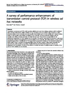
moving to the opposite direction with a maximum speed of 20m/s or 72km/hour. With m of 0.05/s, which corresponds to a maximum speed of 10m/s or 36km/hour in the previous example, 90% of the links are broken before 12s. We observe that the link cannot be maintained for long in these scenarios, which is a typical transportation network scenario. With m = 0.01, it takes 60s for 90% of the links to break. This scenario corresponds to a maximum speed of 2m/s or 7.2km/hour with a transmission range of 200m.

Cumulative Distribution Function

0.8

0.6

0.4

0.2 m = 0.1 m = 0.05 m = 0.01 Simulation 0 0

20

40

60

80

100

t (s)

B. Nodes moving to the same direction Fig. 3. CDF of connectivity period for two adjacent forwarding nodes moving to the opposite direction.

the range of t >

1 m,

P r{Tod > t} =

we have   m− 1  t −m

 +

0

m− 1t

4 1 − t(r − s) dr ds m2

4  1 − t(r − s) dr ds m2

1 t +s

0



0

m



1 = , 30m2 t2 1 1 t} = m2 − 1t 0

(6)

1 − 2(1 − mt)6 = . (7) 30m2 t2 1 , we have and for the range of 0 < t ≤ 2m

4  0  m 1 − t(r − s) dr ds P r{Tod > t} = m2 −m 0 (1 − 2mt)6 − 2(1 − mt)6 + 1 = . (8) 30m2 t2 Combining (7)-(8), P r{Tod ≤ t} = 1 − P r{Tod < t}, the connectivity period when two nodes move to opposite direction can be expressed in closed form as P r{Tod ≤ t}  1 1   for t >  1 − 30m2 t2 ,  m    6  1 1  1 − 1 − 2(1 − mt) , t}, by  P r{Tsd > t} =

m  r  1−t(r−s)

0

0

 =2

0

m r 0



4x3 1 2 2m

dx ds dr

 + 4 1 − t(r − s) m2

0

ds dr, (10)

where 1 − t(r − s) is the distance traveled to break the link, which have been described in previous subsection by (3). We purposefully omit the cases where the node in front is not faster than the node behind from the integration; hence, the limit of the inner integration ends at r. We now derive the CCDF for each specific range of t to remove the x+ operator, hence deriving a simple closed form 1 , we have formulas. For the range of t ≤ m

4 1 − t(r − s) > t} = 2 ds dr m2 0 0  2  6mt + (1 − mt)6 − 1 , = 2 2 30m t 

P r{Tsd

and the CCDF for t >

m r

1 m

(11)

is given by

4 1 − t(r − s) > t} = 2 ds dr+ m2 0 0

4   m r 1 − t(r − s) ds dr 1 m2 r− 1t t 2 1 = − . (12) 5mt 15m2 t2 

P r{Tsd



1 t



r



Similar with the previous subsection, the CDF, P r{Tsd ≤

1 , we have For the range of 0 < t ≤ m  2 2 2

 m 1 − tr+ m t − 3mt + 3 dr = . P r{Ts > t} = m 3 0 (17)

1

Cumulative Distribution Function

0.8

0.6

0.4

For the range of t > 0.2 m = 0.1 m = 0.05 m = 0.01 Simulation 0 0

20

40

60

80

100

t (s)

Fig. 4. CDF of connectivity period for two adjacent forwarding nodes moving to the same direction.

t}, is derived from the CCDF in (11) and (12)    2 1 1   1 − − , for t >  2 t2  5mt 15m m      2   6 P r{Tsd ≤ t} = 1 − 30m2 t2 6mt + (1 − mt) − 1 ,   1   for 0 < t ≤    m   0, otherwise. (13) Fig. 4 shows the connectivity period distribution of two nodes moving to the same direction, comparing the analytical and the simulation results. In this scenario, the analytical results also provide a good match to the simulation results. Using a similar scenario as before, setting the transmission range to 200m, we see that some of the links can be maintained for much longer compared with the case where the nodes are moving away from each other. These links can be maintained because of the speeds of the two adjacent nodes are similar, hence it takes much longer time to break the link. It takes 40s and 80s to break 90% of the links with m equals to 0.1/s (72km/hour) and 0.05/s (36km/hour) respectively. With slower speed, it takes more than 200s to break 90% of the links. C. Node moving away from a stationary node In this scenario, we have only one speed variable, r. The time when the link will break when the distance between the nodes is x can be computed by 1−x . (14) r Thus, we have the equation relating the distance x to the time t and the speed r: x = 1 − tr. (15) t=

Assuming r, we can integrate the density function of x from 0 to 1 − tr to yield the cumulative probability that the link will not break on time less than t. Unconditioning on r, we have the CCDF  2  m 1 − tr+  m  1−tr 2x dx dr = dr. P r{Ts > t} = m m 0 0 0 (16)

P r{Ts > t} =

1 m,

we have  2  1t 1 − tr+ 0

m

dr =

1 . 3mt

Having the CCDF, we can easily derive the CDF by  1 1  for t >   1 − 3mt ,  m  

 1 2 2  m t − 3mt + 3 , 1− P r{Ts ≤ t} = 3  1    for 0 < t ≤   m   0, otherwise.

(18)

(19)

IV. D ISTRIBUTION OF THE S OURCE TO D ESTINATION C ONNECTIVITY P ERIOD In this section, we consider the connectivity period of the end-to-end route from a source to a destination. To derive the distribution of the end-to-end connectivity period, we need to account all the possible combinations of the nodes’ motion. Let kn denotes the direction of the n-th node in the sequence of forwarding nodes that form a route from the source to the destination. Let Vh denotes a vector with h components, {k1 , k2 , . . . kh }. This vector defines the motion of all the forwarding nodes in a 1D MANET (the vector does not contain the source and the destination, as they are stationary). Hence, if we have a source connected to a destination in five hops, the number of forwarding nodes h is equal to 4. As discussed in section II, we have six possible combinations of the two nodes’ motions. Now we define αVh as the number of motion e and motion f in a scenario defined by Vh . Similarly, define βVh as the number of motion c and γVh as the number of motion a in the scenario Vh . We assume that in motion b and motion d, the links will never break as these links will, with high probability, break after the links in the other motion scenarios break. The end-to-end connectivity period is mainly characterized by the motion scenarios which links break the fastest as when any of the link breaks, the whole route breaks; hence, the contribution of motion b, motion d, and the case in motion e and motion f where the node behind is faster to the connectivity period distribution is insignificant. We can easily omit motion b and motion d from the final calculation, but we need a special treatment to remove the special case in motion e and motion f . When two nodes moving to the same direction with uniform speed distribution, the probability that one node is faster than the other is 0.5. The CCDF of the case where the two nodes are moving to the same direction, P r{Tef > t} is then given by P r{Tef > t} = 0.5 · P r{Tsd > t} + 0.5 · 1,

(20)

 P r{Ts2d ≤ t} = 1 −

∀Vh

P r{Tef > t}αVh · P r{Tod > t}βVh · P r{Ts > t}γVh

Cumulative Distribution Function

0.6

0.4

0.2 m = 0.1 m = 0.05 m = 0.01 Simulation 0 10

20

30

40

50

t (s)

Fig. 5.

(21)

the established route between the source and the destination. We show the distribution of end-to-end connectivity period for five hops route in Fig. 5. The figure shows close match between the simulation results and the analytical results, which proves that our approximation does not cause perceptible error. For this scenario, we assume a transmission range of 200m and source is transmitting to a destination that is five hops away. With m of 0.1/s (72km/hour), 90% of the links will break after 3.5s; for m = 0.05/s (36km/hour), it takes 7s for 90% of the links to break. With slower speed of 7.2km/hour), it takes 35s to break 90% of the links.

0.8

0

.

2h

1



CDF of end-to-end connectivity period for five hops route.

where P r{Tsd > t} is given in (11)-(12). Having all the possible combinations of Vh , The CDF of the end-to-end connectivity period is, then, can be computed by (21), where 2h is the number of possible combinations of Vh . The CCDF P r{Tef > t} is given in (20), P r{Tod > t} is computed by (7)-(8), and P r{Ts > t} is given by (17)-(18). The variables αVh , βVh , and γVh are calculated using recursive operations. Consider a vector, Vh , with components {k1 , k2 , . . . , kh−1 , kh }; the last two components of the vector determines the motion scenario for the last hop. Let 0 and 1 mean that the node is moving to the right and to the left respectively2 . With this definition, kh−1 = 1 and kh = 0 describe motion c in Fig. 2c, and kh−1 = kh describe either motion e or motion f . As the source and destination nodes are omitted from Vh , k1 and kh characterize the first and the last hop respectively. The formulas to compute αVh are αV1 = 0 and
αVh−1 + 1, if kh−1 = kh (22) αVh = αVh−1 , otherwise. To compute βVh , we have βV1 = 0 and
βVh−1 + 1, if kh−1 = 1 and kh = 0 βVh = βVh−1 , otherwise. Finally, we compute γVh    0, γVh = 2,   1,

(23)

by γV1 = 1 and if k1 = 1 and kh = 0 if k1 = 0 and kh = 1 otherwise.

(24)

Given the distance between the source and the destination, d, using (1) which indicates the link distance between two forwarding nodes, we can compute the mean number of hops for 2 We use left and right for easy notations to describe the two possible directions in a 1D MANET (note that the considered network might not form a straight line).

V. C ONCLUSION In this paper, we characterize the connectivity period of the route from a source to a destination in 1D MANETs, which implements a reactive routing protocol. We derived the CDF of the connectivity period of each link that connects two adjacent forwarding nodes, as well as the end-to-end connectivity period. We observe that with high mobility nodes, most of the end-to-end routes can only be maintained for few seconds. This result suggests that for high mobility scenarios, each source should maintain more than one active route to reduce the route discovery overhead. Another possibility for vehicular scenarios is to employ better antenna system, which can increase the transmission range of the nodes for higher route reliability. R EFERENCES [1] C. H. Foh and B. S. Lee, “A closed form network connectivity formula for one-dimensional MANETs,” in Proc. IEEE ICC, Paris, France, June 2004, pp. 3739–3742. [2] C. H. Foh, G. Liu, B. S. Lee, B. C. Seet, K. J. Wong, and C. P. Fu, “Network connectivity of one-dimensional MANETs with random waypoint movement,” IEEE Commun. Lett., vol. 9, no. 1, pp. 31–33, Jan. 2005. [3] P. Lassila, E. Hyyti¨a, and H. Koskinen, “Connectivity properties of random waypoint mobility model for ad hoc networks,” in Proc. MedHoc-Net, ˆIle de Porquerolles, France, Mar. 2005. [4] C. Bettstetter, “On the minimum no degree and connectivity of a wireless multi-hop network,” in Proc. ACM MobiHoc, Lausanne, Switzerland, June 2002, pp. 80–91. [5] ——, “Topology properties of ad hoc networks with random waypoint mobility,” in Proc. ACM MobiHoc, Annapolis, Maryland, June 2003. [6] O. Dousse, P. Thiran, and M. Hasler, “Connectivity in ad-hoc and hybrid networks,” in Proc. IEEE Infocom, New York, NY, USA, Mar. 2002. [7] M. Desai and D. Manjunath, “On the connectivity in finite ad hoc networks,” IEEE Commun. Lett., vol. 6, no. 10, pp. 437–439, Oct. 2002. [8] ns2 Network Simulator. [Online]. Available: http://www.isi.edu/nsnam/ns/ [9] C. E. Perkins and E. M. Royer, “Ad-hoc on-demand distance vector routing,” in Proc. IEEE Workshop on Mobile Computing Systems and Applications, New Orleans, Louisiana, USA, Feb. 1999, pp. 90–100. [10] C. Bettstetter, G. Resta, and P. Santi, “The node distribution of the random waypoint mobility model for wireless ad hoc networks,” IEEE Trans. Mobile Comput., vol. 2, no. 3, pp. 257–269, July-Sept 2003.