Nov 13, 2017 - Let us write (i, j) as an abridged notation for xi − xj and define, .... −5 − 2. √. 6X2 + X. The periods of these curves are ε(P0) and ε(P7), ...
Pure and Applied Mathematics Quarterly Volume 4, Number 4 (Special Issue: In honor of Jean-Pierre Serre, Part 1 of 2 ) 1107—1132, 2008
On Local Constants Associated to Arithmetical Automorphic Functions P. Bayer and A. Travesa Dedicated to Jean-Pierre Serre on the occasion of his 80th birthday
Abstract: This article deals with the diophantine nature of the local constants associated to automorphic functions with respect to Fuchsian groups obtained from quaternion algebras. We focus on the canonical model of those curves arising from the quaternion Q-algebra of discriminant D = 6. Introduction Some of the most useful Shimura varieties arise as moduli spaces of abelian schemes with extra structures, in the same way as modular curves are moduli spaces of elliptic curves. In the 1960s, a convenient generalization of the complex multiplication theory for the modular case led Shimura to his theory of canonical models (cf. [21], and [24] for a recent account of the theory). One of the first applications of Shimura curves was provided in [13]. By using fine properties of the N´eron models of the jacobians of modular curves and of Shimura curves associated to quaternion algebras, Ribet was able to prove a very particular case of a deep conjecture of Serre relative to the modularity of (mod p) Galois representations of dimension 2, stated in [19]. As is well known, this was the starting point of Wiles’ proof of Fermat’s Last Theorem (see for instance [20]). At present, very intensive work has been carried out towards a general proof of Serre’s conjecture. Received July 18, 2006. 1991 Mathematics Subject Classification. 11F03, 11G18, 14G35, 30F35. Partially supported by MEC, MTM2006-04895.
1108
P. Bayer and A. Travesa
In spite of their increasing interest, Shimura varieties have been much less studied from an effective point of view, even in dimension one. The reasons appear to be the lack of cusps and, consequently, the lack of Fourier expansions for the automorphic functions involved. In contrast, modular functions possess q-expansions at infinity, being q(z) = e2πiz , which were already known by the classics. In our previous articles [3] and [6], we considered the canonical models of Shimura curves associated to the indefinite quaternion Q-algebra of discriminant D = 6. We expanded their functions at elliptic points and at some distinguished CM-points, called special (SCM for short). This article is concerned with the characterization of the Q-rational functions of the canonical models through their expansions at CM-points. We will restrict our attention to the case of the quaternion Q-algebra of discriminant D = 6. The article is organized as follows: In sections 1 and 2 we summarize the contents of [6] to make our exposition self-contained. The functions defining the canonical models are introduced as solutions of non-linear differential equations of the third order which are set up from fundamental domains. In section 3 we derive an interesting formula which expresses a particular quaternionic automorphic function through quotients of Siegel automorphic forms. In some sense, the formula is analogous to the one expressing the elliptic jfunction in terms of Eisenstein series (cf. [18]). In sections 4 and 5 we introduce some local parameters and obtain explicit expansions at the elliptic points and SCM-points for the functions in section 2. The local parameters adapted to these functions turn out to be of the form µ ¶ z − P eP qP (z) = kP , z−P eP being the order of the isotropy group at P and kP a constant of the same transcendence class as certain products of values of Euler’s gamma function at rational arguments. In section 6 it is proved that the constants kP agree, up to algebraic elements, with some specific constants πd which only depend on the discriminant d of the field of complex multiplication. The identification of the constants at the elliptic points and at the SCM-points involves the use of the Chowla-Selberg formula [17]. The transcendence of the πd -s, for every d, is established by means of a theorem due to Chudnovsky [8]. The results in section 6 are generalized to every CM-point in section 7. Theorem 7.1 illustrates a theorem due to Shimura ([23], theorem 7.1) and shows that
On Local Constants Associated to Arithmetical ...
1109
the transcendental part of kP at a CM-point P agrees with πd . Finally, in theorem 7.3 we stress the arithmetical meaning of the parameters πd that is, that they allow the characterization of the canonical models through series expansions. Contents Introduction
1107
1. Preliminaries on the curve X6
1109
2. Canonical models
1112
3. Uniformizing functions and theta constants
1114
4. Local parameters
1118
5. Local expansions
1122
6. Transcendence classes of adapted local constants at elliptic points and at SCM-points 1125 7. Arithmetical properties of the canonical models
1129
References
1131
1. Preliminaries on the curve X6 Let H6 be the indefinite quaternion Q-algebra of discriminant 6, endowed with a basis {1, I, J, IJ} such that I2 = 3, J2 = −1, IJ = −JI. From the main antiinvolution of the algebra α = x + yI + zJ + tIJ 7→ α = x − yI − zJ − tIJ,
x, y, z, t ∈ Q,
the reduced trace and reduced norm of an element α ∈ H6 are defined by Tr(α) = α + α,
N(α) = αα.
We consider the order O6 := Z [1, I, J, (1 + I + J + IJ)/2] as a representative of the conjugacy class of all maximal orders of H6 . Throughout the paper we fix the embedding of algebras Φ:
H6
−→ ·
x + yI + zJ + tIJ 7→
M(2, √ R) √ ¸ x + y √3 z + t √3 . −(z − t 3) x − y 3
The group of units of O6 of reduced norm equal 1 can be identified with its image Γ6 ⊆ SL(2, R) under Φ. The group Γ6 and its projection Γ6 := Γ6 /{±1}
P. Bayer and A. Travesa
1110
in PSL(2, R) are Fuchsian groups of the first kind without parabolic transformations. The action of Γ6 on the complex upper half-plane H by homographies yields a projective non-singular curve of genus zero. Let us consider an imaginary quadratic field K and suppose that there is an embedding ϕ : K ,→ H6 . The embedding ϕ determines a point P ∈ H, called a CM-point by K, which is fixed under all transformations in√Φ(ϕ(K)). √They include the elliptic points, in which case the field K is either Q( −1) or Q( −3). A CM-point P ∈ H will be called special (SCM) if it is the fixed point of some fractional linear transformation γ ∈ (Φ ◦ ϕ)(OK ) of determinant equal to 6, the discriminant of the algebra. Here OK stands for the ring of integers of K. The theory of canonical models tells us that the curve associated to Γ6 has a canonical model (X6 , j6 ) which is defined over Q. Hence there exists a one to one mapping (cf. section 2) j6 : Γ6 \H → X6 (C). CM-points are relevant since their coordinates j6 (P ) generate class fields over imaginary quadratic fields. A fundamental domain for the action of Γ6 in H, together with its elliptic points and SCM-points, was computed in [1]. This information is collected in table 1 and figure 1.
P1
√ (− 3 + i)/2
P4 (1 + i)/(1 + P7 (1 +
√
√
P2 (−1 + i)/(1 +
3) P5
√
√ ( 3 + i)/2
3) P3 P6
(2 −
√
3)i
i
√ √ √ √ √ 2i)/ 3 P8 (−1 + 2i)/ 3 P0 ( 6 − 2)i/2
Table 1. Vertices of a fundamental domain for X6 and SCM-points Let N (O6 ) be the normalizer of O6 in H6 . The elements of N (O6 ) of positive reduced norm define a subgroup whose image in GL+ (2, R) will be denoted by Γ+ 6. + + The group Γ6 is contained in Γ6 as a normal subgroup and the quotient Γ6 /Γ6 is isomorphic to (Z/2Z)2 . The classes of this quotient are represented by elements wd ∈ O6 of norm d dividing 6. We can take w2 := 1+J, w3 := (−3−I−3J+IJ)/2 and w6 := w2 w3 = −3J + IJ. They define involutions of the curve X6 , denoted ωd . (d)
Together with the curve X6 , we consider its quotients X6 := X6 /hωd i and + X6 := X6 /hωd : d|6i. All these curves fit in a diagram of Galois covers of degree
On Local Constants Associated to Arithmetical ...
1111
P6 P8
c
c
P0
a
P1
a
P7 b
P5
b
P2
P4 P3
Figure 1. Fundamental domain for X6 two:
X6 . ↓ & (2) (3) (6) X6 X6 X6 & ↓ . X6+ . (2)
(3)
Figures 2 and 3 show fundamental domains for the genus zero curves X6 , X6 , (6) X6 , X6+ . P6
P6
b
b
a
b
P0 a
P0 a
P2
a P4
P3
b
P2
P4 P3
(2)
(3)
Figure 2. Fundamental domains for Γ6 and Γ6
The above fundamental domains exhibit particular symmetries. We use some of them to cut fundamental half-domains, that is, half-domains containing all the vertices of a fundamental domain exactly once. Table 2 lists axes of symmetries (2) (3) and polygons defining fundamental half-domains for the curves X6 , X6 , X6 ,
P. Bayer and A. Travesa
1112
P6 P6
b P7 b
a
b
b a
c
P0
P0
a
P5 c
a
P4
P2
P4
P3
(6)
Figure 3. Fundamental domains for Γ6 and Γ+ 6 (6)
X6 , X6+ . The results displayed in table 3 show the angles at the different vertices of the polygons defining the corresponding fundamental half-domains. curve axis of symmetry polygons X6 (P2 , P6 , P4 ) [P2 , P3 , P4 , P6 ] (2) X6 (P3 , P6 ) [P3 , P4 , P6 ] (3) X6 (P2 , P4 ) [P2 , P4 , P6 ] (6) X6 (P0 , P4 , P7 ) [P0 , P4 , P7 , P6 ] X6+ (P0 , P6 ) [P0 , P4 , P6 ] Table 2. Fundamental half-domains
2. Canonical models Since the curves we are dealing with are all of genus zero, there exist au(2) (3) (6) tomorphic functions on H, t6 , t6 , t6 , t6 , t+ 6 , uniquely defined by imposing their values at three vertices of the fundamental half-domains and such that they P0 P2 P3 P4 P6 P7 X6 ∗ π/3 π/2 π/3 π/2 ∗ (2) X6 ∗ ∗ π/4 π/3 π/4 ∗ (3) X6 ∗ π/6 ∗ π/6 π/2 ∗ (6) X6 π/2 ∗ ∗ π/3 π/2 π/2 X6+ π/2 ∗ ∗ π/6 π/4 ∗ Table 3. Angles at the vertices of fundamental half-domains
On Local Constants Associated to Arithmetical ...
1113
t P0 P2 P3 P4 P6 P7 t6 ∗ a 0 1 ∞ ∗ (2) t6 ∗ ∗ 0 1 ∞ ∗ (3) t6 ∗ 0 ∗ 1 ∞ ∗ (6) t6 0 ∗ ∗ 1 ∞ b t+ 6 0 ∗ ∗ 1 ∞ ∗ Table 4. Values of the uniformizing functions at the vertices
(2)
(3)
(6)
uniformize the curves X6 , X6 , X6 , X6 , X6+ . We choose the functions in accordance with table 4. Proposition 2.1. The uniformizing functions defined in table 4 fulfil the following algebraic relations: (2)
(2)
(3)
2 (1) 4t+ 6 t6 = (t6 + 1) .
2 (2) t+ 6 = (2t6 − 1) .
(3) 4t6 (2t6 − 1)2 = (t6 + 1)2 .
(4) t26 = t6 .
(5) 4t6 t6 = (t6 + 1)2 .
(6) t+ 6 + t6 (t6 − 2) = 0.
(7) 2t6 t6 = i(t6 − i)2 .
2 2 (8) 4t26 t+ 6 = (t6 + 1) .
(2)
(3)
(2)
(3)
(6)
(2)
(2) (6)
(6)
(2)
(6)
(6)
(3)
(6)
(6)
(9) (t6 + 1)2 + 4t6 t6 (t6 − 2) = 0. (10) (2t6 − 1)2 + t6 (t6 − 2) = 0. Moreover, we have the following values for the functions: 1 (3) (6) (12) t6 (P0 ) = . (13) b = t6 (P7 ) = 2. 2 (14) a = t6 (P2 ) = −1. (15) t6 (P0 ) = i. (16) t6 (P7 ) = −i. ¤ (2)
(11) t6 (P0 ) = −1.
For a non-constant smooth function f (z), let D(f, z) be its derivative. The automorphic derivative of f is defined as Da(f, z) =
2D(f, z)D3 (f, z) − 3D2 (f, z)2 . D(f, z)4
· ¸ az + b ab For a homographic transformation γ(z) = ,γ = ∈ GL(2, C), we cd cz + d have Da(γ, z) = 0. Conversely, for a non-constant smooth function · ¸ γ(z), the az + b ab , for some γ = ∈ M(2, C). relation Da(γ, z) = 0 implies that γ(z) = cd cz + d The automorphic derivative Da(f, z) of a Γ-automorphic function f (z) is again a Γ-automorphic function. That is to say, for every γ ∈ Γ, z ∈ H the following equality holds: Da(f, γ(z)) = Da(f, z).
P. Bayer and A. Travesa
1114
Proposition 2.2. The functions defined by table 4 satisfy the differential equations Da(t, z) + R(t) = 0, where the rational functions R(t) are listed in table 5. ¤ (2)
(3)
(6)
Theorem 2.3. The functions j6+ , j6 , j6 , j6 : H → P1 (C) given by j6+
:=
(2) j6
t+ 6, √
(3)
j6 := u3 :=
(3)
:= u2 :=
(6)
−3 (1 − 2t6 ), j6 := u6 :=
√
√
(2)
−1
1 + t6
(2)
1 − t6
,
(6)
−3 (1 − t6 ),
and the function j6 : H → P2 (C) given in homogeneous coordinates by j6 := (u3 : u6 : 1) = (u2 : 1 : 1/u6 ) = (1 : 1/u2 : 1/u3 ) (2)
(3)
(6)
define canonical models over Q of the curves X6+ , X6 , X6 , X6 , X6 , respectively. For the last one, we have Q(X6 ) = Q(j6 ) = Q(u3 , u6 ) = Q(u2 , u6 ) = Q(u2 , u3 ). These functions fulfil the following algebraic relations: u23 + u26 + 3 = 0,
u 6 u2 = u3 . ¤
For the proofs of propositions 2.1, 2.2 and theorem 2.3 we refer the reader to [6]. 3. Uniformizing functions and theta constants We consider the alternating bilinear form T(α, β) := Tr(µ α β),
α, β ∈ H6 ,
where µ := −3J + IJ is such that µ2 = −6. The form T is integer valued over O6 . The matrices " √ √ # √ · ¸ · ¸ −1+ 3 −1+ 3 0 −1 −1 + 3 0 2 2 √ η1 = 12 , η2 = 1+√3 −1−√3 , η3 = , η4 = 1 0 0 −1 − 3 2
2
define a symplectic basis in Φ(O6 ) with respect to the bilinear form 1 E(Φ(α), Φ(β)) := T(α, β) 6 (note that 6 equals the positive square root of the Pfaffian of T). Therefore, for a given point z ∈ H, · ¸ z Φ(O6 ) = Z[η1 (z), η2 (z), η3 (z), η4 (z)]. 1
On Local Constants Associated to Arithmetical ...
Curve
function t
vertices angles
−Da(t, z)
X6
t6
[P2 , P3 , P4 , P6 ] [π/3, π/2, π/3, π/2]
27t4 + 74t2 + 27 36t2 (t2 − 1)2
(2)
[P3 , P4 , P6 ] [π/4, π/3, π/4]
135t2 − 142t + 135 144t2 (t − 1)2
(3)
[P2 , P4 , P6 ] [π/6, π/6, π/2]
27t2 − 27t + 35 36t2 (t − 1)2
(2)
t6
(3)
t6
(6)
t6
X6 X6 X6
X6+
(6)
1115
[P0 , P4 , P7 , P6 ] 27t4 − 108t3 + 211t2 − 206t + 108 [π/2, π/3, π/2, π/2] 36t2 (t2 − 3t + 2)2
135t2 − 103t + 108 144t2 (t − 1)2 Table 5. Automorphic derivatives of the functions t+ 6
[P0 , P4 , P6 ] [π/2, π/6, π/4]
We define two period matrices by Ω1 (z) = [η1 (z), η2 (z)], Ω2 (z) = [η3 (z), η4 (z)]. Let ε be the embedding of the Poincar´e upper half-plane H into the Siegel upper half-space H2 of degree 2 defined by ε :H→ H2 z 7→ Ω1 (z)−1 · Ω2 (z), that is
· ¸ √ √ √ 1 1 + 3 − 2 3 z + (1 − 3)z 2 2(1 + z 2 ) √ √ √ √ ε(z) = . 2(1 + z 2 ) −4 3 z 1 − 3 − 2 3 z + (1 + 3)z 2 Henceforth we let Sp(4, R) be the group of the symplectic (4 × 4)-matrices.
We let Γ6 and the transformations Φ(wd ), d|6, act on Φ(O6 ) by multiplication on the right. Since the action of Γ6 preserves the alternating form E, and the elements Φ(wd ) act as symplectic similarities, we obtain two embeddings Ψ : Γ6 → Sp(4, Z),
Ψ+ : Γ+ 6 → Sp(4, R),
which, moreover, are compatible with ε. Hence, there exist well-defined mappings Γ6 \H → Sp(4, Z)\H2 ,
+ Γ+ 6 \H → Sp6 (4, Z)\H2 ,
where Sp+ 6 (4, Z) denotes the subgroup of Sp(4, R) generated by Sp(4, Z) and + + Ψ (Γ6 ).
P. Bayer and A. Travesa
1116
Let x1 , x2 , . . . , x6 be the roots of a sextic a6 X 6 + a5 X 5 + · · · + a0 ,
ai ∈ C.
Let us write (i, j) as an abridged notation for xi − xj and define, in accordance with [12] and [7], the following symmetric functions of the roots: P I2 (a) = a26 (15) (12)2 (34)2 (56)2 , I4 (a) = a46 I6 (a) = a66
P
2 2 2 2 2 2 (10) (12) (23) (31) (45) (56) (64) ,
P
2 2 2 2 2 2 2 2 2 (60) (12) (23) (31) (45) (56) (64) (14) (25) (36) ,
I10 (a) = a10 6
Q
2 i