On Local Optima in Multiobjective Combinatorial Optimization Problems

On Local Optima in Multiobjective Combinatorial Optimization Problems Luis Paquete1 , Tommaso Schiavinotto2 and Thomas St¨ utzle3 1

Universidade do Algarve, Faculdade de Economia, Centro de Sistemas Inteligentes Campus de Gambelas, 8005 Faro, Portugal 2 Signum - Scuola Normale Superiore di Pisa Piazza dei Cavalieri, 7, 56126 Pisa, Italy 3 Universit´e Libre de Bruxelles, CoDE, IRIDIA, CP 194/6, Av. F. Roosevelt 50, 1050 Brussels Abstract. In this article, local optimality in multiobjective combinatorial optimization is used as a baseline for the design and analysis of two iterative improvement algorithms. Both algorithms search in a neighborhood that is defined on a collection of sets of feasible solutions and their acceptance criterion is based on outperformance relations. Proofs of the soundness and completeness of these algorithms are given.

1. Introduction Stochastic local search (SLS) algorithms have been shown to provide high quality solutions for many hard combinatorial problems (Aarts and Lenstra, 1997; Hoos and St¨ utzle, 2004). A central aspect in the development of these methods is the notion of local optimum, that is, a solution that cannot be improved with respect to its neighborhood. In fact, many general-purpose SLS methods (also called metaheuristics) have been designed with the explicit goal to overcome the problems associated with local optimality. SLS algorithms have also been applied with considerable success to multiobjective combinatorial optimization (MOCO) problems (Ehrgott and Gandibleux, 2004). However, different from the single objective counterpart, there is not a widely accepted notion of local optimality in MOCO. This may be a reason why the existing SLS approaches to MOCO problems appear to have been developed often in a more ad-hoc and less directed manner. The notion of local optimum for the single objective case can be extended to MOCO problems by considering sets of solutions. We call the resulting set of local optima a Pareto local optimum set. We first relate the concept Pareto local optimum set to aspects of global and local optima for the single objective case. A negative result is that SLS algorithms for single objective problems are not appropriate for obtaining a Pareto local optimum set. In a next step, we propose two iterative improvement algorithms that search according to a neighborhood that is defined on a collection of sets of solutions, and whose acceptance criterion is based on the better relation defined in (Hansen and Jaszkiewicz, 1998; Zitzler et al., 2003). The first iterative improvement algorithm has, however, the disadvantage of visiting an exponential number of sets of solutions at each iteration of the iterative improvement algorithm. A more restricted version, called Pareto c 2007 Kluwer Academic Publishers. Printed in the Netherlands.

2 local search (PLS), initially proposed and experimentally tested in (Paquete et al., 2002; Paquete et al., 2004), is shown to search for a more interesting and restricted set of solutions. We prove that this algorithm terminates in a specific type of a Pareto local optimum set. In addition, since there can be an exponential number of solutions to be visited, alternatives that restrict the acceptance criterion by using measures for the spread of solutions are discussed. However, we show that some caution must be taken on the type of restrictions to be used since for some choices iterative improvement algorithms can cycle. The article is organized as follows. In Section 2, we introduce notation and discuss the definitions of local optimality we use in this article. Section 3 discusses the relation of these notions to the solutions returned by solving each objective separately. In Section 4, the iterative improvement algorithms are proposed, and Section 5 analyzes PLS with respect to its soundness and completeness. Further extensions and future work are discussed in Section 6. 2. Notation and Definitions 2.1. Multiobjective optimization The following orders in the Euclidean space IRK are considered. Let u and v be vectors in IRK . The strict component-wise order is denoted by u < v, where ui < vi , i = 1, . . . , n; component-wise order by u ≤ v, where u 6= v and ui ≤ vi , i = 1, . . . , n; and weak component-wise order by u ≦ v, where ui ≤ vi , i = 1, . . . , n. Note that if we have that u ≦ v and v ≦ u, then u = v. We consider here the general multiobjective program min

   q1 = F1 (s)  

qK

.. . = FK (s),

(1)

where s belongs to the set S of feasible solutions and min is understood in terms of Pareto optimality. F (s) = (F1 (s), . . . , FK (s)) is the objective function vector of s and K is the number of objectives. Without loss of generality, only minimization is considered. The objective function of a single objective optimization problem is denoted by f (s). We restrict ourselves to combinatorial optimization problems. In the context of optimization, the relation between objective function vectors of two feasible solutions s and s′ is denoted as follows: if F (s) < F (s′ ), then F (s) strictly dominates F (s′ ); if F (s) ≤ F (s′ ), then F (s) dominates F (s′ ); if F (s) ≦ F (s′ ), then F (s) weakly dominates F (s′ ). Finally, F (s) and F (s′ ) are (pairwise) nondominated if F (s) 6≤ F (s′ ) and F (s′ ) 6≤ F (s), and are (pairwise) non weakly dominated if F (s) 6≦ F (s′ ) and F (s′ ) 6≦ F (s). Note that the latter is more restrictive since it implies that F (s) 6= F (s′ ). The same notation is applied when referring to solutions, if the relation holds between their objective function vectors. A solution to Program (1) is one that is globally nondominated, that is, it is not dominated by any other feasible solution. Such a solution is known in

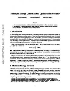
3 the literature as Pareto global optimum. However, there is usually not only one Pareto global optimum but many, and the solution to Program (1) becomes a set of Pareto global optima. A set is a Pareto global optimum set if, and only if, it contains only and all Pareto global optima. Its image in the objective space is called efficient set. Note that several Pareto global optima may have the same objective function vector. Hence, rather than finding the Pareto global optimum set, one may be only interested in one solution for each element of the efficient set. In that case, the strict version of Pareto global optimum set is more appropriate. A set is a strict Pareto global optimum set, if, and only if, it contains only non weakly dominated Pareto global optima and its image in the objective space coincides with the efficient set. A strict Pareto global optimum set is called minimal complete set by Hansen (1979), complete set of alternatives by Emelichev and Perepelista (1992) and strictly Pareto optimal set by Ehrgott (2000). 2.2. Local Optimality An iterative improvement algorithm starts from an arbitrary feasible solution and searches neighbors for better solutions to replace the current one. This neighborhood search is repeated until no improvement is found anymore and the algorithm stops in a local optimum. More formally, let N : S 7→ 2S be a neighborhood function that associates a set of feasible solutions N (s) to every feasible solution s. A feasible solution s′ ∈ N (s) is also called a neighbor of s. The solution s is a local optimum with respect to N if, and only if, there is no s′ ∈ N (s) such that f (s′ ) < f (s). Note that different iterative improvement algorithms can be defined in dependence of the criterion used for searching an improving neighbor. The notion of local optimum can be easily extended to MOCO in terms of Pareto optimality by adapting the notion of Pareto global optimum. In (Paquete et al., 2004), a feasible solution s is called a Pareto local optimum with respect to a neighborhood N , if, and only if, there is no s′ ∈ N (s) such that F (s′ ) ≤ F (s). For the same reasons presented above for defining a Pareto global optimum set, Paquete et al. (2004) defined a set S ′ ⊆ S to be a Pareto local optimum set with respect to a neighborhood N if, and only if, all solutions in S ′ are Pareto local optima with respect to N . (An analogous definition of Pareto local optimum set is given in (Deb, 1999).) Note, however, that such a set may contain dominated solutions and therefore, if nothing else is said, we require the Pareto local optimum set to have only solutions that are pairwise nondominated. Finally, an extension of this definition to non weakly dominated solutions was introduced in (Paquete and St¨ utzle, 2006). Fig. 1 illustrates the image of a Pareto local optimum set with non weakly dominated solutions in the objective space (two minimizing objectives) by black points, where neighbors are connected by edges. It can be seen that no neighbor (represented by gray points) dominates any of the black points and that the black points are pairwise non weakly dominated. Note that a Pareto global optimum is also a Pareto local optimum, independent of the neighborhood N . A Pareto global optimum set is a Pareto local

4

Figure 1. The set of black points forms a non weakly dominated Pareto local optimum set. The gray points are neighbors to each element of that set.

optimum set with nondominated solutions and a strict Pareto global optimum set is a Pareto local optimum set with non weakly dominated solutions. In this sense, these notions are analogous to the relationship of the notions of local optimum and global optimum in the single objective case. Putting this analogy further to the level of algorithms, it is natural to require an iterative improvement algorithm for MOCO problems to terminate once a Pareto local optimum set with only non weakly dominated solutions is found. Remark: In the remainder of this paper, we will, for conciseness, refer to a Pareto local optimum set with only non weakly dominated solutions simply as a Pareto local optimum set.

3. Local Optima and Pareto Local Optima Given the analogies between local optima for the single- and multiobjective case, a first question is whether applying iterative improvement algorithms to each objective of a MOCO problem separately can be used for obtaining a Pareto local optimum set. In general, the answer is no and we will illustrate these results using the Multiobjective Traveling Salesman Problem (MOTSP). In the MOTSP are given n cities and distance vectors in IN K for each pair of cities. The goal is to find a set of Hamiltonian tours that is minimal with respect to the notion of Pareto optimality. This problem is known to be NP-hard since its single objective version is NP-hard (Serafini, 1986). The first negative result states that there may be cases in which a Pareto global optimum is not a local optimum for any single objective of a MOCO problem. This is shown by the following example. EXAMPLE 3.1. Consider the MOTSP instance with 5 cities that is taken from (Emelichev and Perepelitsa, 1991).1 In Figure 2 is given a biobjective MOTSP 1

Emelichev and Perepelitsa (1991) proposed a generalization of this instance as an example of an MOTSP instance that has unsupported Pareto global optima.

5 (1, 5)

a

b (2, 2) (5, 1)

d e

c

Figure 2. Graph of the MOTSP instance for Example 3.1. All the edge weight vectors are (5, 5) except for the ones labeled explicitly.

instance (the edges without label have weight vectors (5, 5)). The Pareto global optimum set (Sg ) and the corresponding image in the objective space (Og ) are presented in the following table: solution

Sg

Og

s1

(a, b, d, e, c) (a, b, e, d, c) (a, b, c, e, d) (a, b, c, d, e) (a, c, b, d, e) (a, c, b, e, d)

(18, 22)

s2 s3 s4 s5 s6

(18, 22) (21, 21) (21, 21) (22, 18) (22, 18)

Consider the 2-exchange neighborhood, where for a given solution s, all neighbors can be obtained by replacing two edges from s with two different edges not present in s. For this neighborhood, any solution with objective function vector (21, 21) is not a local optimum for any component of the objective function vector since there is a better neighbor for each objective. For example, the solution s4 has two better neighbors: solution s2 with respect to the first objective (by removing the edges (b, c) and (e, a) and adding the edges (b, e) and (c, a) in s4 ) and s5 with respect to the second objective (by removing the edges (a, b) and (c, d) and adding the edges (a, c) and (b, d) in s4 ). The following example shows that a locally optimal solution with respect to at least one objective of the MOCO problem may not be a Pareto local optimum. EXAMPLE 3.2. Figure 3a gives a biobjective MOTSP instance (the edges that are not present have each distance vector component larger than 2). The Pareto global optimum set is {(a, g, e, b, d, c, f )}, the tour indicated by bold edges, and the efficient set is {(7, 8)}. Under the same 2-exchange neighborhood from the previous example, the sequence s = (a, b, c, d, e, f, g), which is indicated in Figure 3b with straight lines, has an objective value vector (8, 12) and it is a locally

6 a (1, 1)

(1, 2)

(1, 1)

g (1, 2)

f

(1, 1)

(1, 1)

(1, 1)

(1, 1)

(1, 2)

(1, 2)

(1, 2)

c

f

(2, 2)

a

d

b (1, 2) (1, 1)

(1, 1)

e

(1, 2)

g

b

(1, 2)

a

c

(1, 1)

(1, 2)

(1, 1)

e

(2, 2)

d

b

Figure 3. An MOTSP instance (a) and a local optimum (b) for Example 3.2.

optimal tour for the first component. However, this sequence is not a Pareto local optimum since it is weakly dominated by the sequence (a, b, e, d, c, f, g) obtained by removing the edges (b, c) and (e, f ) from s, and adding the edges (b, e) and (c, f ) (the latter two edges are dashed in Figure 3b) with an objective value vector (8, 10). These two examples give a negative answer to the initial question posed in this section, that is, solutions returned by applying an iterative improvement algorithm to each objective may not result in a Pareto local optimum set. However, an acceptance criterion that accepts sets of solutions can, in fact, identify Pareto local optima. Two variants are discussed in the next two sections.

4. A basic iterative improvement algorithm for MOCO One common approach to solve MOCO problems is to use the (weak) componentwise ordering when comparing neighboring solutions (Knowles and Corne, 2000; Angel et al., 2004b; Paquete et al., 2004). In that case, the acceptance criterion is to accept a neighbor if it is non (weakly) dominated; since in the local search process we can expect to have more than one solution for which this holds, an additional data structure, which is usually called archive, is used to maintain the current set of solutions. How do these two features, component-wise acceptance criterion and the usage of an archive, relate to our notions of Pareto local optimum set? To answer this question we have to define an analogy to iterative improvement algorithms for the single objective case. In fact, in the literature there are almost no iterative improvement algorithms for MOCO problems that stop in a set of solutions that cannot be improved locally, an exception being the Pareto local search (PLS) algorithm proposed in (Paquete et al., 2004). In this section, we define a basic iterative improvement algorithm for MOCO problems that is based on a general neighborhood between sets of solutions and a dominance relation between sets of points. In the next section, we discuss the relationship

7 of the outcomes of PLS to the outcomes of this basic iterative improvement algorithm. Certainly, a suitable stopping criterion for a basic iterative improvement algorithm for MOCO problems is to terminate once a Pareto local optimum set is found. Hence, such an algorithm should, at each iteration, select a set of non Sweakly dominated solutions and work on a set of solutions. We define US ′ = s∈S ′ N (s) for a given arbitrary neighborhood function N and a set S ′ of feasible solutions. Then, a natural neighborhood of S ′ , identified by Υ(S ′ ), is the power set of S ′ ∪ US ′ , that is, ′

Υ(S ′ ) = 2S ∪US ′ . The next step is to define an acceptance criterion for sets of solutions that are neighbors with respect to Υ. For this task, the outperformance relations proposed in (Hansen and Jaszkiewicz, 1998) and later extended in (Zitzler et al., 2003) are useful. Given two arbitrary point sets A and B in a K-dimensional objective space, the following relations are introduced: ◦

1. A < B if every b in B is strictly dominated by at least one a in A, i.e., A strictly dominates B; ◦

2. A ≤ B if every b in B is dominated by at least one a in A, i.e., A dominates B; ◦

3. A
B if every b in B is weakly dominated by at least one a in A and A 6= B, i.e., A is better than B; ◦

4. A ≦ B if every b in B is weakly dominated by at least one a in A, i.e., A weakly dominates B; ◦

◦

◦

5. A k B if neither A ≦ B nor B ≦ A, i.e., A and B are incomparable. ◦

◦

◦

◦

Moreover, A < B ⇒ A ≤ B ⇒ A
B ⇒ A ≦ B (Zitzler et al., 2003). Figure 4 illustrates these relations between sets of points in the objective space with two minimizing objectives in some particular cases. In Plot 1, any black point is strictly dominated by a white one. Plot 2 shows that there is a black point (the minimum with respect to F1 ) that is dominated (but not strictly) by another two white points. The remaining black points are strictly dominated by some white point. Plot 3 shows that all black points are weakly dominated by white points, although not all black points (the gray points belong to both sets) are dominated, and hence, the two sets are different. In Plot 4, both sets are equal and the white points weakly dominate the black points and vice-versa. Finally, the plot on the bottom shows two sets that are incomparable, i.e., one can neither say that all black points dominate the white ones nor vice-versa. Based on the neighborhood Υ and on any of the outperformance relations above, local search algorithms can now be defined. In fact, depending on the particular relation chosen, different outcomes can be expected. Consider first

8 F2

F2

8

8

6

6

4

4

2

2 2

4

6

8

2

F1

1. A < B F2

8

8

6

6

4

4

2

2 4

6

8

F1

8

F1

2. A ≤ B

F2

2

4 ◦

◦

6

8

2

F1

◦

◦

4

6 ◦

4. A ≦ B (and B ≦ A)

3. A
B F2 8 6 4 2 2

4

6 ◦

8

F1

5. A k B Figure 4. Illustration of relations between a set A (white points) and a set B (black points) of nondominated objective value vectors. A gray point belongs to both sets. Note that each plot shows a special case that cannot be classified w.r.t. the preceding relation. For example, ◦

A ≦ B is true for plots 1 to 4, but the special case in the plot 4 cannot be classified with ◦

◦

◦

respect to the relations