On Making Directed Graphs Eulerian arXiv ... - Semantic Scholar

On Making Directed Graphs Eulerian

arXiv:1101.4283v2 [cs.DM] 18 Feb 2011

Manuel Sorge

Diplomarbeit zur Erlangung des akademischen Grades Diplom-Informatiker

Friedrich-Schiller-Universität Jena Institut f¨ ur Informatik Theoretische Informatik I / Komplexitätstheorie

Betreuung: Dipl.-Inf. René van Bevern Prof. Dr. Rolf Niedermeier Dipl.-Inf. Mathias Weller

¨ Uberarbeitete Version Eingereicht von Manuel Sorge, geb. am 28.04.1986 in Zittau. Jena, den 21. Februar 2011

Zusammenfassung. Einen gerichteten Graphen nennt man Eulersch, wenn er eine Tour enth¨ alt, die jede gerichtete Kante genau einmal besucht. Wir untersuchen das Problem Eulerian Extension (EE) in dem ein gerichteter Multigraph G und eine Gewichtsfunktion gegeben ist, und gefragt wird, ob G durch Hinzuf¨ ugen gerichteter Kanten, deren Gesamtgewicht einen Grenzwert nicht u ¨berschreitet, Eulersch gemacht werden kann. Dieses Problem ist motiviert durch Anwendungen im Erstellen von Fahrplänen f¨ ur Fahrzeuge und Abfolgepl¨ anen f¨ ur Fließbandarbeit. Allerdings ist das Problem EE NP-schwer; deshalb analysieren wir es mit Hilfe von Parametrisierter Komplexität. Die Parametrisierte Komplexit¨ at eines Problems hängt nicht nur von der Eingabelänge, sondern auch von anderen Eigenschaften der Eingabe ab. Diese Eigenschaften nennt man “Parameter”. Dorn et al. [10] zeigten, dass EE in O(4k n4 ) Zeit gelöst werden kann. Hier bezeichnet k den Parameter “Anzahl der gerichteten Kanten, die hinzugef¨ ugt werden m¨ ussen”. In dieser Arbeit analysieren wir EE mit den (kleineren) Parametern “Anzahl c der verbunden Komponenten im Eingabegraph” und “Summe b aller indeg(v) − outdeg(v) u ur die dieser Wert ¨ber alle Knoten v f¨ positiv ist”. Wir zeigen dass es einen Lösungsalgorithmus f¨ ur EE gibt, dessen 2 Laufzeit den Term 4c log(bc ) als einzigen superpolynomiellen Term beinhaltet. Um diesen Algorithmus zu erhalten, machen wir mehrere Beobachtungen u ¨ber die Mengen gerichteter Kanten, die dem Eingabegraph hinzugef¨ ugt werden m¨ ussen, um ihn Eulersch zu machen. Aufbauend auf diesen Beobachtungen geben wir außerdem eine Reformulierung von EE in einem Matchingkontext. Diese Matchingformulierung k¨ onnte ein bedeutendes Werkzeug sein, um zu klären, ob EE in Laufzeit gel¨ ost werden kann, deren superpolynomieller Anteil nur von c abh¨ angt. Außerdem betrachten wir Vorverarbeitungsalgorithmen polynomieller Laufzeit f¨ ur EE, und zeigen, dass diese keine Instanzen erzeugen können, deren Gr¨ oße polynomiell nur von einem der Parameter b, c, k abhängt, es sei denn coNP ⊆ NP/poly.

1

Abstract. A directed graph is called Eulerian, if it contains a tour that traverses every arc in the graph exactly once. We study the problem of Eulerian Extension (EE) where a directed multigraph G and a weight function is given and it is asked whether G can be made Eulerian by adding arcs whose total weight does not exceed a given threshold. This problem is motivated through applications in vehicle routing and flowshop scheduling. However, EE is NPhard and thus we use the parameterized complexity framework to analyze it. In parameterized complexity, the running time of algorithms is considered not only with respect to input length, but also with respect to other properties of the input—called “parameters”. Dorn et al. [10] proved that EE can be solved in O(4k n4 ) time, where k denotes the parameter “number of arcs that have to be added”. In this thesis, we analyze EE with respect to the (smaller) parameters “number c of connected components in the input graph” and “sum b over indeg(v) − outdeg(v) for all vertices v in the input graph where this value is positive”. We prove that there is an algorithm for EE whose running time is 2 polynomial except for the term 4c log(bc ) . To obtain this result, we make several observations about the sets of arcs that have to be added to the input graph in order to make it Eulerian. We build upon these observations to restate Eulerian extension in a matching context. This matching formulation of EE might be an important tool to solve the question of whether EE can be solved within running time whose superpolynomial part depends only on c. We also consider polynomial time preprocessing routines for EE and show that these routines cannot yield instances whose size depends polynomially only on either of the parameters b, c, k unless coNP ⊆ NP/poly.

2

Contents 1 Introduction 1.1 Preliminaries . . . . . . . . . . . . . . . . . . . . . . 1.1.1 Parameterized Algorithmics . . . . . . . . . . 1.1.2 Graphs . . . . . . . . . . . . . . . . . . . . . 1.2 Problems, Variants, Relationships . . . . . . . . . . . 1.2.1 Relations to the Rural Postman Problem . . 1.2.2 Relations to the Hamiltonian Cycle Problem 1.2.3 Constrained Eulerian Extensions . . . . . . . 1.3 Our Work . . . . . . . . . . . . . . . . . . . . . . . .

. . . . . . . .

. . . . . . . .

2 Connected Components 2.1 Structure of Eulerian Extensions . . . . . . . . . . . . . 2.2 Simplification through Advice . . . . . . . . . . . . . . . 2.2.1 Computing Realizations of Hints . . . . . . . . . 2.2.1.1 The minpath Function . . . . . . . . . 2.2.1.2 Removing Cycles from an Advice . . . 2.2.2 The Impact of Advice . . . . . . . . . . . . . . . 2.2.2.1 Reducing EE to EECA . . . . . . . . . 2.2.2.2 Reducing EEA to EE . . . . . . . . . . 2.2.3 An Efficient Multivariate Algorithm for EECA . 2.3 From Eulerian Extension to Matching and back . . . . . 2.3.1 Conjoining Bipartite Matching . . . . . . . 2.3.1.1 NP-Hardness . . . . . . . . . . . . . . . 2.3.1.2 Tractability on Restricted Graphs . . . 2.3.2 The Relationship between Eulerian Extension and 2.3.2.1 Reducing EECA to CBM . . . . . . . 2.3.2.2 Islands of Tractability for EE . . . . . . 2.3.2.3 Reducing CBM to EEA . . . . . . . . 2.4 Discussion . . . . . . . . . . . . . . . . . . . . . . . . . .

. . . . . . . .

. . . . . . . .

. . . . . . . .

. . . . . . . .

. . . . . . . .

. . . . . . . . . . . . . . . . . . . . . . . . . . . . . . . . . . . . . . . . . . . . . . . . . . . . . . . . . . . . . . . . . Matching . . . . . . . . . . . . . . . . . . . .

4 5 5 7 11 12 13 15 15 17 19 25 26 26 28 30 31 32 36 39 39 40 44 48 49 53 54 58

3 Incompressibility 59 3.1 Switch Set Cover . . . . . . . . . . . . . . . . . . . . . . . . . 59 3.2 Switch Set Cover is Or-Compositional . . . . . . . . . . . . . 60 3.3 Lower Bounds for Problem Kernels . . . . . . . . . . . . . . . . . 64 4 Conclusion

71

3

Chapter 1

Introduction The notion of Eulerian graphs dates back to Leonhard Euler. In 1735, he solved the question of whether there is a tour through the city of Königsberg such that every bridge is crossed once and only once [14]. The term “Eulerian tour” has been coined for such a tour. At Euler’s time, the city of Königsberg had seven bridges across the river Pregel and it turned out that an Eulerian tour did not exist. Later, in the nineteenth century, a railway bridge has been built, making such a tour feasible [30]. In this thesis, we study the problem where, given a city, it is asked what is a minimum-cardinality set of bridges that have to be built such that the city allows for an Eulerian tour? Typically, one aims for minimizing the costs for bridge-building. Thus, we mainly focus on a weighted version of this problem. Also, instead of ordinary bridges, we consider bridges that only allow traffic in one way. We call the problem of making a city allow for an Eulerian tour by building one-way bridges, weighted according to a cost function, Eulerian Extension. The problem of Eulerian Extension is also well-motivated through wholly different approaches. Recently, it has been shown by H¨ ohn et al. [21] that some sequencing problems can be solved with Eulerian Extension. An example for such a sequencing problem is “no-wait flowshop”, where a schedule of jobs is sought, each processing on a fixed succession of machines, such that no waiting time occurs for any job between the processing on two subsequent machines. Such problems arise, for instance, in steel production [20]. Another problem that has strong ties to Eulerian Extension is Rural Postman. There, a postman’s tour in a city is sought such that a given subset of streets in the city is serviced. Dorn et al. [10] have proven that Rural Postman is equivalent to Eulerian Extension. Rural Postman can be applied, for example, in routing of snow plowing vehicles [13]. Unfortunately, Eulerian Extension is NP-hard, and thus it is likely not to be solvable within time polynomial in the input size. Thus, we analyze Eulerian Extension using the parameterized-complexity framework. That is, we consider running times not only depending on the input size, but also depending on other properties of the input—called parameters. A problem is called fixed-parameter tractable for a specific parameter if there is an algorithm whose exponential running-time portion depends only on this parameter. For instance, Dorn et al. [10] have proven that Eulerian Extension is fixed-parameter tractable 4

with respect to the parameter k = “number bridges that have to be built”. They have shown that Eulerian Extension can be solved with an algorithm that has running time O(4k n4 ). In this work, we consider smaller parameters for Eulerian Extension. In particular, we look at the number of “islands” the input city consists of and a more technical parameter which we introduce later. By islands we mean districts in the city that are completely cut off from other districts and cannot be reached via bridges. On the positive side, despite Eulerian Extension being NP-hard, we are able to derive algorithms for this problem whose exponential running time portion depends only on these two, presumably small, parameters. On the negative side, we observe that preprocessing Eulerian Extension such that the size of the resulting instances is bounded by polynomials in these parameters likely is not possible. Our work is organized as follows: In Section 1.1, we gather a common knowledge base by recapitulating basic notions of graph theory and parameterized algorithmics. Section 1.2 treats previous work on Eulerian Extension and the related problem of Rural Postman. There we also give an NP-hardness proof for Eulerian Extension for illustrative purposes. In Chapter 2, constituting the main part of this work, we consider structural properties of Eulerian Extension and derive an efficient algorithm. We also restate the problem in a matching context. This matching formulation might become a stepping stone to solve the question of whether Eulerian Extension is fixed-parameter tractable with respect to the parameter “number of islands in the city” we have sketched above. Chapter 3 contains our considerations with regard to preprocessing routines for Eulerian Extension. There, it is shown that no polynomial-time data reduction rules exist that reduce an instance to a polynomial-size problem kernel unless coNP ⊆ NP/poly. Finally in Chapter 4, we give a brief summary of our results and give directions for further research.

1.1

Preliminaries

We assume the reader to be familiar with the basics of set theory, logic, algorithm analysis, and computational complexity. They are covered, for example, by Cormen et al. [7] and Arora and Barak [1].

1.1.1

Parameterized Algorithmics

Many problems of practical importance are NP-hard. Thus, it is widely believed that for these problems there is no algorithm whose running time is bounded by a polynomial in the input size. However, in practice sometimes the phenomenon can be observed, that instances of such problems are indeed solvable within reasonable time. The reason for this is that some algorithms can be analyzed such that their super-polynomial running time portion depends only on some property of the input instances. If such a property, called “parameter”, is not dependent on the input size and if it is “small” in practical instances, then it becomes feasible to solve even big instances of NP-hard problems. The notion of parameters also gives rise to a method measuring the effectiveness of data reduction rules: If the rules reduce an instance such that its size is bounded by

5

polynomials depending only on the parameter, we may assume that the reduction rules perform well in practice. The design of algorithms exploiting small parameters is treated in Niedermeier [27]. However, it is likely that not every problem admits such an algorithm for every possible parameter. In this regard, complexity-theoretic approaches are presented in Downey and Fellows [11] and Flum and Grohe [16]. We use the parameterized complexity framework in our analysis of Eulerian Extension and give some basic definitions of parameterized algorithms and complexity here. Problems and Parameterizations. Let Σ be an alphabet. A parameterization is a polynomial-time computable function κ : Σ∗ → N. A parameterized problem over Σ is a tuple (Q, κ) where Q ⊆ Σ∗ and κ is a parameterization. For an instance I ∈ Σ∗ of a parameterized problem (Q, κ) we also call κ(I) the parameter. A parameterized problem (Q, κ) is called fixed-parameter tractable with respect to κ, if there is an algorithm that, given an instance I ∈ Σ∗ , decides whether I ∈ Q in time at most f (κ(I)) · p(length(I)). Here, f : N → N is a computable function and p is a polynomial. Search Tree Algorithms. A straightforward way to prove a problem fixedparameter tractable is to employ search tree algorithms. A search tree algorithm recursively divides an instance of a problem into a number of new instances. It divides the instances, until they are solvable within polynomial time. If both the recursion depth of the algorithm and the number of new instances generated from each instance is bounded by the parameter, then we obtain an algorithm whose superpolynomial time-portion is bounded by some function depending only on the parameter. Thus, the algorithm is a witness to the fixed-parameter tractability of the problem. Since search tree algorithms often terminate early, are easily parallelized and often allow for many performance tweaks, they often form relevant practical algorithms for NP-hard problems. Problem Kernels. Problem kernels are often used to give a guarantee of efficiency for data reduction rules. Let (Q, κ) be a parameterized problem. A reduction rule for (Q, κ) is a mapping r : Σ∗ → Σ∗ such that (1) r is polynomial-time computable, (2) for every I ∈ Σ∗ it holds that I ∈ Q if and only if r(I) ∈ Q, and (3) κ(r(I)) ≤ κ(I). Statement (2) is called the correctness of the rule. A reduction to a problem kernel for (Q, κ) is a reduction rule r : Σ∗ → Σ∗ such that for every I ∈ Σ∗ it holds that length(r(I)) ≤ h(κ(I)), where h is a computable function. If h is a polynomial, then we call r a reduction to a polynomial-size problem kernel. Parameterized Reductions. Let (Q, κ), and (Q0 , κ0 ) be two parameterized problems. A parameterized many-one reduction from (Q, κ) to (Q0 , κ0 ) is a mapping r : Σ∗ → Σ∗ such that for every I ∈ Σ∗ (1) r(I) is computable in time at most f (κ(I))·p(length(I)), where f : N → N is a computable function and p a polynomial, (2) r(I) ∈ Q0 if and only if I ∈ Q, and (3) there is a computable function g : N → N such that κ0 (r(I)) ≤ g(κ(I)).

6

Statement (2) is called the correctness of the reduction. If the function f is a polynomial in statement (1) we call r a parameterized polynomial-time manyone reduction. If the function g in statement (3) is a polynomial, we call r a polynomial-parameter many-one reduction. A parameterized Turing reduction from (Q, κ) to (Q0 , κ0 ) is an algorithm with an oracle to Q0 that, given an instance I ∈ Σ∗ , (1) decides whether I ∈ Q, (2) has running time at most f (κ(I)) · p(length(I)), where f : N → N is a computable function and p a polynomial, and (3) there is a computable function g : N → N such that for every oracle query I 0 ∈ Σ∗ posed by the algorithm it holds that κ(I 0 ) ≤ g(κ(I)). Parameterized Complexity. It is assumed that not all parameterized problems are fixed-parameter tractable. To distinguish the various degrees of (in-)tractability, there is a multitude of complexity classes. We briefly introduce the classes FPT ⊆ W[1] ⊆ W[2] ⊆ . . . ⊆ W[P ] ⊆ XP. For a brief introduction to parameterized intractability and the W-hierarchy see Chen and Meng [6], for comprehensive works see Downey and Fellows [11] or Flum and Grohe [16]. The class FPT contains all parameterized problems that are fixed-parameter tractable. The class W[t], t ∈ N contains all problems that are parameterized many-one reducible to the satisfiability problem for circuits with depth at most t and an AND output gate, parameterized by the weight of the sought truth assignment—that is the number of variables that are assigned true. The class W[P ] contains all parameterized problems (Q, κ) such that it can be decided whether a word I ∈ Σ∗ is contained in Q in at most f (κ(I)) · p(length(I)) time, using a Turing machine that makes at most h(κ(I)) · log(length(I)) nondeterministic steps. Here, f, h : N → N are computable functions and p is a polynomial. The class XP contains all parameterized problems (Q, κ) for which there is a computable function f such that it can be decided whether I ∈ Σ∗ is contained in Q in time at most length(I)f (κ(I)) + f (κ(I)). A parameterized problem (Q, κ) is assumed to be fixed-parameter intractable, if it is hard for the class of problems W[1]. That is, all parameterized problems in W[1] are parameterized many-one reducible to (Q, κ). Hardness for W[1] can be shown via a parameterized many-one reduction from a W[1]-hard parameterized problem. Such a problem is, for instance, Independent Set parameterized by the size of the sought independent set k: Independent Set Input: A graph G = (V, E) and an integer k. Question: Is there a vertex subset S ⊆ V such that k ≤ |S| and G[S] contains no edges?

1.1.2

Graphs

We now recapitulate some basic notions of graph theory. We oriented our definitions towards the ones given by Bang-Jensen and Gutin [2]. Other books on graph theory include Diestel [8] and West [29]. We also give some non-canonical

7

definitions for notions that we frequently use; especially in the “Connectivity” and “Degree and Balance” paragraphs below. A directed multigraph G is a tuple (V, A), where V is a set, A is a multiset and for every a ∈ A : a = (u, v) ∈ V × V ∧ u 6= v.1 We sometimes denote V by V (G) and A by A(G). Elements in V are called the vertices of G and elements in A are called the arcs of G. We denote |V | by n and |A| by m where it is appropriate. A vertex v ∈ V and an arc (u, w) ∈ A are called incident if u = v or w = v. Two vertices u, v ∈ V are called adjacent or neighbors if there is an arc a ∈ A such that u, v and a are incident. Let B be an arc set. We define the directed multigraph G + B as (V, A ∪ B). Subgraphs. Any directed multigraph (V 0 , A0 ) such that V 0 ⊆ V and A0 ⊆ A is called a subgraph of G. Let V 0 ⊆ V be a vertex set. The graph G[V 0 ] := (V 0 , B) where B = A ∩ V 0 × V 0 is called the vertex-induced subgraph of G with respect to V 0 . Let A0 ⊆ A be an arc-set. The graph GhA0 i := (W, A0 ) where W = {v ∈ V : ∃a ∈ A0 : v and a are incident} is called the arc-induced subgraph of G with respect to A0 . Walks, Trails, and Paths. A walk is an alternating sequence v1 , a1 , v2 , . . . , vk−1 , ak−1 , vk of vertices vi ∈ V and arcs aj ∈ A such that aj = (vj , vj+1 ) for all 1 ≤ j ≤ k − 1. A subwalk of a walk w is a consecutive subsequence of w beginning and ending with a vertex. We say that a walk traverses a vertex v (an arc a) if the vertex v (the arc a) is contained in the corresponding sequence. We say that a walk w traverses a vertex set (arc set), if all vertices (arcs) in the set are traversed by w. The length of a walk is the number of arcs it traverses. The first vertex of a walk w is called the initial vertex and the last vertex is called the terminal vertex. The initial and terminal vertices are also called the endpoints of w. We say that a walk is closed if its initial and terminal vertices are equal. A trail in the graph G is a walk that traverses every arc of G at most once. A path in the graph G is a trail that traverses every vertex of G at most once. A closed trail that traverses every vertex of G at most once except for its initial and terminal vertices is called a cycle. We sometimes abuse notation and identify walks with their corresponding arc sets or their arc-induced subgraphs. Graphs and Orientations. A multigraph G is a tuple (V, E), where V is a set, E is a multiset and for every e ∈ E : e ⊆ V ∧ |e| = 2. We sometimes denote V by V (G) and E by E(G). Vertices, edges, incidence, (vertex- or edge-induced) subgraphs, walks, trails and paths are defined analogously to the definitions for multigraphs. Directed graphs (digraphs for short) and graphs are the special cases of multigraphs that comprise arc or edge sets instead of multisets, respectively. A (directed) graph is called complete if it contains all possible edges (arcs). Let G = (V, E) be a (directed) graph and let G0 = (V, E 0 ) be a complete (directed) graph. The complement graph of G is the graph G = (V, E), where E = E 0 \ E. 1 We exclude “self-loops” (v, v) ∈ A here, because they are not meaningful in the context of Eulerian extensions.

8

4

17 5

1

2

14

10

3 15

13 7

6

16 8 19

9 12

11

18 20

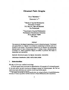
Figure 1.1: A directed graph G (vertices 1 through 20, solid arcs), and its components (encircled and shaded in gray). Furthermore, a number of trails is shown that traverse vertices of G (dashed arcs). The mapping CG () maps both the trails traversing the vertices 5, 14 and 17, 2, respectively, to trail in CG that is represented by the solid line. The trails traversing the vertices 12, 9, 8, 19, 6 and 8, 20, 18, 19, 6, 3, respectively, both map to the trail represented by the dotted lines.

A directed multigraph is said to be an orientation of a multigraph G if it can be obtained from G by substituting every edge {u, v} by either the arc (u, v) or the arc (v, u). The underlying multigraph of a directed multigraph G is the uniquely determined multigraph G0 such that G is an orientation of G0 . Drawing Graphs. We draw a directed multigraph by drawing circles for vertices, sometimes drawing their names inside the circle, and by drawing arrows with the head at the circle corresponding to the vertex u for arcs (v, u). Multigraphs are drawn by drawing circles for vertices and by drawing lines between the corresponding circles for edges. Connectivity. A (directed) multigraph G is said to be connected if for every pair of vertices u, v ∈ V (G) there is a path with the endpoints u, v in (the underlying multigraph of) G. A maximal vertex set C ⊆ V (G) such that G[C] is connected is called a connected component of G. We sometimes abuse notation and identify connected components C with their vertex-induced subgraphs G[C]. When it is clear from the context we denote connected components simply by components. By the component graph CG of G we denote the complete graph that has a vertex for every connected component of G. Consider a trail t that traverses only vertices of G and the trail s in CG that is obtained from t as follows: for every connected component C of G, substitute every maximum length subtrail t0 of t such that V (t0 ) ⊆ C by the vertex in CG that corresponds to C. We denote the underlying trail of s by CG (t). For an example on connected components and the CG () mapping, see Figure 1.1. 9

Degree and Balance. Let G = (V, A) be a directed multigraph. The indegree (outdegree) of a vertex v ∈ V denoted by indeg(v) (outdeg(v)) is |{(u, v) ∈ A}| (|{(v, u) ∈ A}|). The balance of v, denoted by balance(v), is indeg(v) − outdeg(v). In directed multigraphs, a vertex v is called balanced if balance(v) = 0. Let G = (V, E) be a multigraph. The degree of a vertex v ∈ V denoted by deg(v) is |{{u, v} ∈ E}|. In multigraphs, a vertex v is called balanced if deg(v) is even. Let G = (V, E) be a (directed) multigraph. We denote the set of unbalanced + vertices by IG . If G is directed, we denote {v ∈ V : balance(v) > 0} by IG − and {v ∈ V : balance(v) < 0} by IG . Eulerian Graphs and Extensions. A closed trial in a (directed) multigraph G is said to be Eulerian, if it traverses every edge in E(G) (arc in A(G)) exactly once and every vertex in V (G) at least once.2 A (directed) multigraph is called Eulerian, if it contains an Eulerian trail. The following theorem holds. Theorem 1.1.1. A (directed) multigraph is Eulerian if and only if it is connected and every vertex is balanced. A version of Theorem 1.1.1 that is restricted to graphs is due to Euler, a proof for the generalized version above can be found in Bang-Jensen and Gutin [2]. We call an edge multiset (arc multiset) E such that G + E is Eulerian an Eulerian extension for G. Edges (arcs) contained in E are called extension edges (extension arcs). Vertex Partitions and Bipartite Graphs. Let G = (V, A) be a (directed) multigraph. A family of sets P = {C1 , . . . , Ck } is called a vertex partition of G, Sk if V = i=1 Ci and Ci ∩ Cj = ∅ for all 1 ≤ i < j ≤ k. The sets Ci , 1 ≤ i ≤ k are called cells of the partition P . A graph G = (V1 ] V2 , E) is called a bipartite graph, if {V1 , V2 } is a vertex partition of G and for every e = {u, v} ∈ E : u ∈ V1 ∧ v ∈ V2 .3 Matchings. Let G = (V, E) be a graph. A set M ⊆ E is called a matching in G or of the vertices in G, if for every e, f ∈ E : e ∩ f = ∅. A matching M is called perfect if for every vertex v ∈ V there is an edge in M that is incident to v. The following theorem holds: Theorem 1.1.2 (Hall’s condition). A bipartite graph G = (V1 ] V2 , M ) has a perfect matching, if and only if U ≤ N (U ) for every U ⊆ V1 . Here, N (U ) denotes the set of all neighbors of U . A proof for Theorem 1.1.2 can be found in Bang-Jensen and Gutin [2]. 2 Note that there seem to be two equally well-accepted definitions of Eulerian trails: The definitions with and without the additional vertex condition. We chose the one with the vertex condition here, because it makes it easier to deal with connected components that consist only of one vertex. Algorithmically, problems according to both formulations are easily inter-transformable. 3 In this regard we use the symbol ] to indicate a disjoint union of the vertex sets.

10

Eulerian extension on unweighted graphs Connected Disconnected √ √ Undirected m n m n m log(n)(m + n log(n)) Directed nm log(n) Table 1.1: Complexity results regarding unweighted Eulerian extension problems. The number of edges in complement graphs of graphs with m edges is denoted by m. Running times in big-O notation. The result for undirected and directed graphs have been obtained by Boesch et al. [4] and Dorn et al. [10], respectively.

1.2

Problems, Variants, Relationships

Eulerian graphs are interesting by themselves from a graph-theoretic point of view. However, they also bear intuitive and practical applications. In this section we introduce various problems regarding Eulerian graphs, their complexity if it is known, and point out relations to other problems. As we will see later in this section, some natural problems translate into the problem of making a given graph Eulerian by adding edges or arcs, respectively. In these problems it is beneficial to add as few edges as possible, or to add edges such that their total weight is as low as possible. This translates into the following problem formulation: Eulerian Extension (EE) Input: A directed multigraph G = (V, E) and a weight function ω : V × V → [0, ωmax ] ∪ {∞}. Question: Is there an Eulerian extension for G of weight at most ωmax ? The problem of Unweighted Eulerian Extension is EE where every arc in V × V has weight 1. Natural variants of these problems can be derived by substituting undirected multigraphs, directed graphs or graphs for multigraphs in the problem description. As we will also see, the complexity of problems regarding weighted Eulerian extensions depends heavily on the connectedness of the input graph. So, connectedness makes for another intuitive distinction in these problems. Polynomial-time Solvable Variants. Table 1.1 shows polynomial running time results for unweighted Eulerian extension problems on graphs. For unweighted multigraphs, Dorn et al. [10] obtained linear-time algorithms for both the directed and undirected case. These algorithms work regardless of whether the input multigraph is connected or disconnected. Polynomial-time solvability has also been proven for the unweighted and connected variants shown in Table 1.2. Fixed-Parameter Tractability. In general, EE is NP-hard. We recapitulate two NP-hardness proofs in the following subsections. However, Dorn et al. [10] have proven EE to be fixed-parameter tractable with respect to a slightly complicated parameterization: Let E(G, ω) be the set of all Eulerian extensions E for the directed multigraph G with weight ω(E) ≤ ωmax according to the weight function ω.

11

Weighted, connected Eulerian extension Graphs Multigraphs Undirected Directed

|IG |3 log(|IG |) m log(n)(m + n log(n))

|IG |3 log(|IG |) n3 log(n)

Table 1.2: Complexity results regarding weighted Eulerian extension problems on connected graphs. The number of edges in complement graphs of graphs with m edges is denoted by m. Recall that IG denotes the set of not balanced vertices in the input graph. Running times in big-O notation. These results have been obtained by Dorn et al. [10]. Theorem 1.2.1. Eulerian Extension parameterized by k = max{|E| : E ∈ E(G, ω)} is solvable in O(4k n4 ) time. Note that the according parameterization is likely not polynomial-time computable. This calls for the trick to encode the parameter in the corresponding language Q of the parameterized problem. The parameter then has to be checked for correctness by any algorithm that decides Q.

1.2.1

Relations to the Rural Postman Problem

In this section, we briefly review the many-one reductions from Eulerian Extension (EE) to the Rural Postman problem and back, given by Dorn et al. [10]. From these reductions we get parameterized equivalence with respect to parameters that motivate our choice of parameters for EE. The Rural Postman problem is defined as follows. Rural Postman (RP) Input: A directed graph G = (V, A), a set R ⊆ A of required arcs and a weight function ω : A → [0, ωmax ] ∪ {∞}. Question: Is there a walk W in G such that W traverses all arcs in R and ω(W ) ≤ ωmax ? Dorn et al. [10] observed that RP parameterized by the “number of arcs in the sought walk” and EE parameterized by “number of arcs in the sought Eulerian extension” are equivalent.4 We take a brief look at their construction here and observe a further parameterized equivalence. The main idea in both reductions is to exploit the following observation. Observation 1.2.1. Let G be a directed graph and let W be a multiset of arcs in G. There is a closed walk in G that uses exactly the arcs W if and only if the directed multigraph (V (G), W ) is Eulerian. With Observation 1.2.1 it is easy to see that the following two constructions are polynomial-time many-one reductions from RP to EE and from EE to RP, respectively. Construction 1.2.1. Let the directed graph G = (V, A), the required arc set R and the weight function ω : V ×V → [0, ωmax ]∪{∞} constitute an instance of RP. 4 The

actual parameters are slightly more complicated, but this intuition suffices here.

12

Construct an instance of EE by defining the directed multigraph G0 := (V, R) and a weight function ω 0 : V × V → [0, ωmax − ω(R)] ∪ {∞} by ( ω(a), a ∈ A ∧ ω(a) ≤ ωmax − ω(R), 0 ω := ∞, otherwise. Construction 1.2.2. Let the directed multigraph G = (V, A) and the weight function ω : V × V → [0, ωmax ] ∪ {∞} constitute an instance of EE. Construct an instance of RP by defining the directed graph G := (V, V × V ), the required 0 arc set R := A, the weight function ω 0 = ω and the maximum weight ωmax := ωmax + ω(R). In the search for suitable parameters for EE, we observed the following. Intuitively, we expect the number of connected components in GhRi to be small in practical instances. For instance, consider a postman’s tour in a city that comprises a number of suburbs. The number of streets that have to be serviced in each of the suburbs is expected to be much higher than the streets in-between, thus forming connected components in each suburb. We also expect the sum of positive balances of all vertices in GhRi to be small: This sum is at most proportional to the number of required arcs, and we assume this number to be small compared to n in practice. With regard to EE, the following observation is of much interest. Observation 1.2.2. Let G be the input digraph and R the required arcs in an instance of RP. Let G0 be the input graph in an instance of EE. Construction 1.2.1 and Construction 1.2.2 are polynomial-time polynomial-parameter many-one reductions with respect to the parameters (i) number of connected components in GhRi and number of connected components in G0 , and/or (ii) sum of all positive balances in GhRi and sum of all positive balances in G0 . This motivates the analysis of EE with respect to these two parameters. In this regard, Frederickson [18] has proven the following theorem. Theorem 1.2.2. Rural Postman can be solved in O(n3 n2c−2 /c!) time, where c is the number of connected components in GhRi—the graph G being the input graph and R the set of required arcs. From this theorem it immediately follows that RP parameterized by the number of components in GhRi is in XP and thus, by Observation 1.2.2, EE parameterized by the number of components in the input graph also is in XP.

1.2.2

Relations to the Hamiltonian Cycle Problem

In this section we observe that the difficulty of solving Eulerian Extension (EE) depends on the number of components in the input graph. This is done using a reduction from the Hamiltonian Cycle problem. A natural question is, whether the difficulty of solving EE depends only on the number c of components, that is, whether EE is fixed-parameter tractable with respect to the parameter c. We attack this question in Chapter 2, especially Section 2.3.

13

This section also shows that the parameter “sum of all positive balances of vertices in the input graph” for EE will likely not yield fixed-parameter tractability. The Hamiltonian Cycle problem is defined as follows. Definition 1.2.1. Let G be a directed graph. A cycle in G is called Hamiltonian if it traverses every vertex in G exactly once. Hamiltonian Cycle (HC) Input: A directed graph G. Question: Is there a Hamiltonian cycle in G? Orloff [28] notes that the complexity of RP seems to depend on the number of connected components in GhRi, where G is the input graph and R is the set of required arcs. In a way, Lenstra and Kan [24] proved this statement by giving a reduction from the NP-hard [23] HC problem such that the number of components in GhRi in the RP instance is exactly the number of vertices in the HC instance. In this section, we give a reduction from HC to EE illustrating that the same is true for EE. The main idea of the reduction is that any Eulerian extension for EE has to connect all connected components in the input graph. Thus, we model every vertex by a connected component consisting of two vertices that are connected by two arcs: One arc in either direction. To model edges in the instance of RP, we utilize the weight function and choose ωmax accordingly to ensure that every feasible Eulerian extension is a cycle. Construction 1.2.3. Let the directed graph G0 = (V 0 , A0 ) constitute an instance of RP. Construct an instance of EE as follows: Define the directed multigraph G = (V, A) by V := V 0 × {0, 1} and A := {((v, 1), (v, 0)), ((v, 0), (v, 1)) : v ∈ V 0 }. Set the maximum weight ωmax := |V 0 | and define the weight function ω by ( 1, a = ((u, 0), (v, 0)) ∧ (u, v) ∈ A0 , ω(a) := ∞, otherwise. It is easy to see that this construction is correct using the following observation: Observation 1.2.3. Any Eulerian extension E for G with ω(E) ≤ ωmax is a cycle. Proof. Since E has to connect |V 0 | connected components in G, it contains at least |V 0 | − 1 arcs. The Eulerian extension E cannot contain a maximum-length trail that is open, since there are no unbalanced vertices in G. For sake of contradiction assume that E contains three arcs that are incident to one vertex v in G. Then, to connect the remaining connected components in G via a closed trail, E has to contain at least |V 0 | − 3 arcs. However, then v is still not balanced and E has to contain at least one additional arc, totalling in |V 0 | + 1 arcs. Thus, by contradiction, every vertex in G has at most two incident arcs in E and thus E is a cycle. 14

Thus, Construction 1.2.3 is correct and we have that the difficulty in solving EE depends on the number of components in the input graph. But the reduction given by Construction 1.2.3 also gives the following observation. Observation 1.2.4. EE parameterized by the sum of all positive balances of vertices in the input graph is not contained in XP, unless P = NP. Proof. Observe that all vertices in the graph G produced by Construction 1.2.3 are balanced. If EE parameterized by the sum b of all positive balances of vertices in the input graph was in XP, in particular all instances with b = 0 were solvable within polynomial time. Thus, HC would be solvable within polynomial time.

1.2.3

Constrained Eulerian Extensions

A natural modification of Eulerian extension problems is to give constraints on the set of edges or arcs that can be added to the input graph in order to make it Eulerian. Note for example that in Eulerian Extension on graphs we can regard the condition that the input graph has to remain a graph with the added edges as a constraint on the allowed edges (that is multiedges are forbidden). Thusly constrained problems might also be interesting in practice. For instance, Höhn et al. [21] observed that the following class of constrained Eulerian extension problems has applications to sequencing problems: d-Dimensional Eulerian Extension Input: A directed graph G = (V, A), where V ⊂ Qd . Question: Is there an Eulerian extension E for G such that for every (u, v) ∈ E it holds that u ≥ v component-wise? However, H¨ ohn et al. [21] also have proven that d-Dimensional Eulerian Extension is NP-complete. We model such constraints on the extension edges in such problems as instances of Eulerian Extension by simply defining the weight function accordingly—assigning forbidden arcs or edges the weight ∞, and setting the maximum weight to a large enough value. We use d-Dimensional Eulerian Extension as a helper problem in Chapter 3. In order to deal conveniently with the arc constraints, we introduce some notation at this point. Definition 1.2.2. Let ω be a weight function assigning weights [0, ωmax ] ∪ {∞} to arcs. An arc a is called allowed with respect to ω if ω(a) < ∞. If the weight function is clear from the context, then we simply say that the arc is allowed.

1.3

Our Work

In recent research by Dorn et al. [10] the problem Eulerian Extension (EE) has been shown to be fixed-parameter tractable with respect to the parameter k = “number of arcs in the sought Eulerian extension”.5 In this work we initiate a more fine-grained analysis of the EE problem by considering parameters that are upper bounded by k. In particular, we study the parameterizations “number c 5 The actual parameter is slightly more complicated—see page 11—but the intuition of the number of needed extension arcs suffices here.

15

Parameterized complexity results for Eulerian Extension Parameter Known New k c b, c

∈ FPT : 4k ∈ XP —

no polykernel ∈ W[P ], no polykernel 2 ∈ FPT : 4c log(bc ) , no polykernel

Table 1.3: Overview on parameterized complexity results for EE regarding various parameters. Fixed-parameter tractability results include the superpolynomial term of the corresponding algorithm. Known results: The fixed-parameter tractability result for parameter k is due Dorn et al. [10]. The XP-result for parameter c is due Frederickson [18] (see Subsection 1.2.1). New results: The fixed-parameter tractability result for the combined parameter b, c is shown in Theorem 2.2.3 and Corollary 2.2.1. The W[P ]-result for parameter c follows from Observation 2.3.1 and Theorem 2.3.5. The non-existence of polynomial-size problem kernels is shown in Theorem 3.3.2 and its corollaries. of components in the input graph” and “sum b of all positive balances of vertices in the input graph”. Since any Eulerian extension E for a multigraph has to produce a connected graph, it holds that |E| ≥ c − 1 and thus k ≥ c − 1 . Also, any Eulerian extension E has to balance all vertices in the given multigraph, that is, for every vertex v with balance d > 0, it has to contain at least d outgoing arcs. Hence it holds that |E| ≥ b and thus k ≥ b. Table 1.3 gives a compact overview over the new and known results regarding EE. EE parameterized only with b is already NP-hard when b = 0: Consider the reduction we give in Subsection 1.2.2 to prove NP-hardness for EE. This reduction produces instances with b = 0. Also, the question whether EE is fixedparameter tractable when parameterized by c is a long-standing open question which arose implicitly in research by Frederickson [18, 19]. His work implies that EE is polynomial-time solvable for every constant value of c (see Subsection 1.2.1). However, his algorithm does not imply fixed-parameter tractability and this question seems to be hard to answer. Nevertheless, in Chapter 2 we show that when parameterizing with both b and c EE becomes fixed-parameter tractable. Pursuing the question whether EE is fixed-parameter tractable with only the parameter c, we restate EE in the context of matchings in Chapter 2 and show that the problem Conjoining Bipartite Matching is parameterized equivalent to EE. Using the matching formulation we obtain a fixed-parameter tractability result for a restricted class of EE when parameterized by c. We also consider preprocessing routines for EE in Chapter 3. In this regard, we show that d-Dimensional Eulerian Extension does not admit a polynomial problem kernel with respect to the parameter k. The result also transfers to the parameters b, c and the more general problem EE.

16

Chapter 2

Connected Components The main results given in this chapter are an efficient algorithm for Eulerian 2 Extension (EE) with running time in O(4c log(bc ) n2 (b2 + n log(n)) + n2 m) and the parameterized equivalence of EE parameterized by c and Conjoining Bipartite Matching. Here, c is the number of components and b is the sum of all positive balances in the input graph, that is for the input graph G, it P is b = v∈I + balance(v). The equivalence to the matching problem also yields G

4

an algorithm for a restricted form of EE with O(2c(c+log(2c )) (n4 + m)) running time. The latter result represents some partial progress to answer the question of whether EE is fixed-parameter tractable with respect to the parameter c. We first make some observations about Eulerian extensions in Section 2.1 which expose that every Eulerian extension corresponds to a specific structure that has an intimate relationship to the connected components of the input graph. This then leads to a modified problem derived from EE in Section 2.2. There we consider the problems Eulerian Extension with Advice (EEA) and Eulerian Extension with Minimal Connecting Advice (EECA) where the structure of the sought Eulerian extensions is made explicit in the input. These restricted problems seem to be easier to tackle and we derive an algorithm with O(4c log(b) n2 (b2 + n log(n)) + n2 m) running time for EECA. Using observations about the relationship between EE and EECA we derive an 2 algorithm for EE running in O(4c log(bc ) n2 (b2 + n log(n)) + n2 m) time. In Section 2.3 we introduce Conjoining Bipartite Matching (CBM) and show that it is tractable on some restricted graph classes. We give parameterized reductions from EE to CBM and from CBM to EE using some intermediary problems that we introduce in Section 2.2. This then yields the parameterized equivalence of CBM and EE. As simple corollaries, we derive fixed-parameter tractability of EE with respect to parameter c on some restricted input instances. The reductions also yield some results for intermediary problems, for example a problem kernel for EECA that has size polynomial in b and c. Consult Figure 2.1 and Table 2.1 for an overview on the reductions given in this chapter and the tractability results obtained.

17

pT

EE

EECA

pt-pp-m

3SAT pt-pp-m

pt-pp-m

EEA

pt-m CBM

Figure 2.1: Schematic overview on the reductions given in this chapter. The label “pT” indicates a parameterized Turing reduction, the label “pt-pp-m” indicates a polynomial time polynomial parameter many-one reduction, and the label “pt-m” indicates a classical polynomial time many-one reduction. The reductions from and to EE are covered in Section 2.2. The reductions from and to CBM are given in Section 2.3.

Problem a

CBM CBMb EECA EEA EEc EEd EE

Tractability results Result n+m 2j(j+1) n + n3 4c log(b) n2 (b2 + n log(n)) + n2 m b2 c vertex kernel 16c log(c) (cn4 + m) 4 2c(c+log(2c )) (n4 + m) 2 4c log(bc ) n2 (b2 + n log(n)) + n2 m

Proposition Corollary 2.3.1 Lemma 2.3.4 Theorem 2.2.3 Corollary 2.3.6 Corollary 2.3.3 Corollary 2.3.4 Corollary 2.2.1

Table 2.1: Overview on tractability results given in this chapter. All values in big-O notation. Here, j denotes the parameter “join set size” in CBM instances. This parameter corresponds to the parameter “number of components” in EE instances in reductions we give in this chapter. a When

the the c When the d When the b When

input graph is a forest. bipartite input graph has maximum degree two in one of its cells. allowed arcs “resemble” a forest. allowed arcs “resemble” a vertex-disjoint union of cycles.

18

+

− Figure 2.2: Examples of a closed maximum length trail (left, solid arcs) and an open maximum length trail (right, solid arcs) in an Eulerian extension (solid arcs). Arcs belonging to the input graph are dashed. Observe that the vertex + + − is the only vertex in IG and the vertex − is the only vertex in IG .

2.1

Structure of Eulerian Extensions

In this section, we show that we can assemble a minimum-weight Eulerian extension for a graph G using trails that are of restricted structure, and bound the length and number of “long” trails by polynomials in the number of components in G. To this end, we consider trails in Eulerian extensions. We investigate preprocessing routines for instances of EE—namely, we split vertices (Transformation 2.1.1) and use shortest-path preprocessing (Transformation 2.1.2)—that allow us to modify any valid Eulerian extensions such that we can make assumptions about their trails without increasing the weight of the extensions. In this section, we frequently use the component graph CG of a graph G and the mapping CG (t) of trails t in G to trails in CG . These are defined on page 9 in Section 1.1. The main result of this section is as follows. Theorem 2.1.1. Let G be a directed multigraph with c connected components. Let G and the weight function ω : V ×V → [0, ωmax ]∪{∞} constitute an instance of Eulerian Extension that is preprocessed using Transformation 2.1.1 and Transformation 2.1.2. Then, there is a set S := {t1 , . . . , tk } of pairwise edgedisjoint paths and cycles each in the graph (V, V × V ) such that Sk (i) i=1 A(ti ) is an Eulerian extension of minimum weight for G, (ii) each ti ∈ S contains at most c + 1 vertices, (iii) in S there are at most c(c − 1)/4 paths and cycles containing more than one arc, + − (iv) the number of paths in S is at most |IG | = |IG |, (v) for ti 6= tj ∈ S of length at least two CG (ti ), and CG (tj ) are edge-disjoint, (vi) the graph defined by the union of all trails CG (t1 ), . . . , CG (tn ) without their initial vertices does not contain a cycle. In this section, let G = (V, A) be a directed multigraph, let E be an Eulerian extension for G—that is G + E := (V, A ∪ E) is Eulerian—and let the function ω : V × V → [0, ωmax ] ∪ {∞} be a weight function. Observation 2.1.1. A maximum-length trail in an Eulerian extension for a + − graph G either is closed or starts in IG and ends in IG . Proof. Consider the initial vertex vA and terminal vertex vΩ of a trail t in the Eulerian extension E. The vertices vA and vΩ are balanced in G + E. 19

Assume that vΩ is not balanced in G. Every time t traverses vΩ , it uses one arc in E that enters vΩ and one that leaves it. This implies that vΩ 6= vA because vΩ is balanced in G + E and thus there is an odd number of arcs in E incident to vΩ (recall that t is of maximum length). Since t ends in vΩ , this also − + implies that vΩ ∈ IG . Analogously we get that vA ∈ IG . Now assume that vΩ is balanced in G. Since t cannot be extended, it already uses every arc incident to vA and vΩ . However, if vΩ is not equal to vA , there are more arcs entering vΩ than leaving vΩ in E. This means that vΩ is not balanced in G + E which is a contradiction. Figure 2.2 illustrates Observation 2.1.1. Preprocessing Routines. There is a preprocessing routine introduced by Dorn et al. [10] that ensures that every vertex has balance between −1 and 1. This later helps to give a bound on very short trails in Eulerian extensions. Transformation 2.1.1 (Splitting Vertices). Let the graph (G = (V, A), the weight function ω and the maximum weight ωmax ) constitute an instance of EE. Compute a new instance as follows: Search for a vertex v with | balance(v)| > 1, introduce a new vertex u. If balance(v) > 0, choose an arbitrary arc (w, v), delete it and add the arc (w, u). Proceed analogously, if balance(v) < 0. Add the arcs (u, v), (v, u). Finally, define a new weight function ω 0 for each pair of vertices x, y ∈ V as follows.  ∞, x = u, y = v ∨ x = v, y = u    ω(v, y), x = u ω 0 (x, y) =  ω(x, v), y = u    ω(x, y), otherwise Lemma 2.1.1. Transformation 2.1.1 is correct, that is, it maps yes-instances and only yes-instances to yes-instances. Also, Transformation 2.1.1 can be applied exhaustively in O(n2 m) time. When applied exhaustively, the resulting instance contains only vertices v with | balance(v)| ≤ 1. Proof. The last statement of the lemma is clear. Concerning the running time, we can iterate over every vertex v ∈ V (O(n) time), check if it has high absolute balance (O(m) time) and, if so, perform the weight function update (O(n) time) and perform the local modifications (O(1) time) for every “excess arc” incident to v (there are at most m many). In total, this is O(n2 m) time. To prove the correctness, we only have to examine one application of Transformation 2.1.1: Let (G0 = (V 0 , A0 ), ω 0 , ωmax ) be an instance of EE where Transformation 2.1.1 has been applied once at vertex v yielding the new vertex u. Given an Eulerian extension for the input graph G, we can obtain an Eulerian extension for G0 of the same weight by modifying an arc a ∈ E incident to v appropriately such that it starts or ends in u. If we are given an Eulerian extension for G0 , at least one arc in it has to be incident to u and thus we can obtain an Eulerian extension for G by modifying it to start or end in v. We can apply a further preprocessing routine to make some further observations about trails in Eulerian extensions:

20

Transformation 2.1.2 (Shortest-Path Preprocessing). For an input instance of EE consisting of the graph G = (V, A), the weight function ω and the maximum weight ωmax , derive a new instance by computing a new weight function ω 0 as follows: ω 0 (u, v) := weight of a shortest path from u to v in the graph (V, V × V ). Lemma 2.1.2. Transformation 2.1.2 is correct—that is, it maps yes-instances and only yes-instances to yes-instances—and can be applied in O(n3 ) time. Proof. It is clear that for any Eulerian extension E of G it holds that ω 0 (E) ≤ ω(E), making any feasible Eulerian extension in the original instance also one for the modified instance. Now let E be an Eulerian extension for G with ω 0 (E) ≤ ωmax . We get an Eulerian extension E 0 for G with ω(E 0 ) ≤ ωmax by exchanging every arc a = (u, v) ∈ E with ω 0 (a) < ω(a) by the set of arcs of a shortest path from u to v in the graph (V, V × V ) with respect to the weight function ω. Using Dijkstra’s algorithm we can compute in O(n2 ) time the weights of the shortest paths between one vertex v and any other in G and update the weight function accordingly. Doing this for every vertex in G takes O(n3 ) time. Shortest-path preprocessing and splitting vertices enables us to make a range of useful observations regarding trails in Eulerian extensions. In the following we assume any instance of Eulerian Extension to be preprocessed using Transformation 2.1.1 and Transformation 2.1.2. In the subsequent sections, we use this preprocessing in parameterized algorithms and reductions. Thus, we need to know whether it is parameter-preserving. This is the case, as the following observation shows. Observation 2.1.2. The number of components and the sum of all positive balances of vertices in an instance of EE are invariant under Transformation 2.1.1 and Transformation 2.1.2. Shortcutting Trails in Eulerian Extensions. Using Transformation 2.1.2, we can define the following transformation that operates on trails of an Eulerian extension. Transformation 2.1.3. Let E be an Eulerian extension of G, let t be a trail in the graph (V (G), E) and let s be a subtrail of t where s has the initial vertex vA and the terminal vertex vΩ . Obtain a new trail t0 by substituting the edge (vA , vΩ ) for s in t and derive a new arc set E 0 by substituting A(t0 ) for A(t) in E. Define shortcut(E, t, s) := (E 0 , t0 ). Figure 2.3 illustrates Transformation 2.1.3. Lemma 2.1.3. Let shortcut(E, t, s) = (E 0 , t0 ) where the trail s has initial vertex vA and terminal vertex vΩ . The following statements hold: (i) ω(E 0 ) ≤ ω(E). (ii) Every vertex in V (s) is balanced in G + E 0 . (iii) If every vertex of s except vA and vΩ is contained in a connected component of G that also contains a vertex of t0 , then the arc set E 0 is an Eulerian extension for G. 21

vA

vΩ

Figure 2.3: Example of an application of Transformation 2.1.3. Solid arcs and dotted arcs belong to t, dotted arcs to s and the dashed arc is substituted for the dotted arcs in t0 .

Proof. Statement (i) is trivial because of the implicitly transformed weight function (Transformation 2.1.2). By substituting (vA , vΩ ) for s, every vertex on s except vA and vΩ looses one indegree and one outdegree. Hence, augmenting G with E 0 results in a graph without unbalanced vertices (statement (ii)). For statement (iii) it remains to show that the graph (V (G), A ∪ E 0 ) is connected: If every vertex of s except vA and vΩ is contained in a connected component of G that also contains another vertex of t0 , then augmenting G with E 0 results in a connected graph, making E 0 an Eulerian extension for G (Theorem 1.1.1). Observation 2.1.3. For any Eulerian extension E of G = (V, A) there is an Eulerian extension E 0 of at most the same weight such that any trail with arcs in E 0 visits every vertex at most once. Proof. Assume that in the Eulerian extension E there is a trail t that visits v ∈ V more than once. Then there is a subtrail s = (u, (u, v), v, (v, w), w) ˆ t0 ) = shortcut(E, t, s). By Lemma 2.1.3, E ˆ is an of t with u, w ∈ V . Let (E, Eulerian extension for G because t0 still visits v (one time less than t). If we recursively shortcut edges in trails in E until every such trail visits any vertex at most once, we obtain an Eulerian extension E 0 . By Lemma 2.1.3, ω(E 0 ) ≤ ω(E). Observation 2.1.3 allows us to assume trials in Eulerian extensions to be cycles when they are closed and paths otherwise. Observation 2.1.4. For any Eulerian extension E of G, there is an Eulerian extension E 0 of at most the same weight such that for any path p and any cycle c in E 0 such that p and c are edge-disjoint and have length at least two the following statements hold: (i) p and c do not successively visit two vertices contained in exactly one connected component of G. (ii) p and c do not visit one connected component of G twice except for the initial and terminal vertex. (iii) p and c have length at most the number of connected components of G. Proof. The proof for (i) and (ii) is similar to the proof of the observation above. Again we can shortcut edges and obtain an Eulerian extension of at most the same weight. Statement (iii) directly follows from (i) and (ii). 22

r

t t0 Figure 2.4: Gray objects represent components of G. Shown are two trails r (top) and t (bottom, solid and dashed arcs) in an Eulerian extension. The trails CG (r), CG (t) share two vertices. The dashed arcs represent a subtrail s0 of t as in Lemma 2.1.4 and thus we can obtain a path t0 (bottom, solid and dotted arcs) replacing t, while maintaining connectedness and balance of all vertices.

Shortcutting and Component Graphs. We can further extend our observations by looking at component graphs CG and the mapping of trails t in G to trails CG (t) in CG . Recall these definitions stated on page 9 in Section 1.1. The following lemma is a generalization of statement (iii) in Lemma 2.1.3. Lemma 2.1.4. Let E be an Eulerian extension of G, let t, r be trails in the directed multigraph (V (G), E) such that the trails CG (r) and CG (t) are not vertexdisjoint. Furthermore, let s be a subtrail of t in the directed multigraph (V (G), E) such that CG (s) is a subtrail of CG (r). Let s0 be a subtrail of t such that s is a subtrail of s0 and s traverses exactly one vertex less than s0 . Set (E 0 , t0 ) = shortcut(E, t, s0 ). Then E 0 is an Eulerian extension for G. Proof. Lemma 2.1.3 shows that the vertices in G + E 0 are balanced. It remains to show that the resulting graph is connected: Any connected component that is traversed by s is also traversed by u. The trails CG (u) and CG (t0 ) still share a vertex and thus G + E 0 is connected. Lemma 2.1.4 leads to the following Observation 2.1.5, which is illustrated in Figure 2.4. Observation 2.1.5. For any Eulerian extension E of G there is an Eulerian extension E 0 of at most the same weight such that for any two edge-disjoint trails t1 , t2 in E 0 it holds that CG (t1 ), CG (t2 ) either are vertex-disjoint, share at most one vertex, or share only their initial and terminal vertices. Proof. This follows directly from Lemma 2.1.4 by shortcutting subtrails that are shared by two such trails in CG . We can improve this even to the following. Observation 2.1.6. For any Eulerian extension E of G there is an Eulerian extension E 0 of at most the same weight such that for any set ofSedge-disjoint n trails {t1 , . . . , tn } in E 0 it holds that the edge-induced graph CG h i=1 CG (ti )0 i 0 does not contain a cycle as subgraph, where CG (ti ) is CG (ti ) without the initial vertex. 23

Proof. By Observation 2.1.3 we Sn may assume that S := {t1 , . . . , tn } are paths or cycles. Assume that CG ( i=1 CG (ti )0 ) contains a cycle c and that S is minimal with respect to this property. Let e ∈ ti be an arbitrary edge on c. There is a subtrail s of ti such that CG (s) traverses e and at least one edge not belonging to c—recall that CG (ti )0 is CG (ti ) without the initial vertex. Shortcutting s maintains balance of every vertex (statement (ii), Lemma 2.1.3) and connectedness, because afterwards CG (ti ) is not vertex-disjoint from c. Since an edge is removed from c, it is a path after shortcutting s. Sn Iterating the shortcutting for every cycle in the graph CG ( i=1 CG (ti )0 ) eventually removes every cycle after a finite amount of steps, because obviously the statement of the lemma holds true, if t1 , . . . , tn have length one, and because in every step the number of arcs in E decreases by at least one. We use Observation 2.1.6 in forthcoming Subsection 2.2.2 to efficiently derive the structure of a suitable Eulerian extension for a given graph. We are now ready to prove Theorem 2.1.1. Theorem 2.1.1. Let G be a directed multigraph with c connected components. Let G and the weight function ω : V ×V → [0, ωmax ]∪{∞} constitute an instance of Eulerian Extension that is preprocessed using Transformation 2.1.1 and Transformation 2.1.2. Then, there is a set S := {t1 , . . . , tk } of pairwise edgedisjoint paths and cycles each in the graph (V, V × V ) such that Sk (i) i=1 A(ti ) is an Eulerian extension of minimum weight for G, (ii) each ti ∈ S contains at most c + 1 vertices, (iii) in S there are at most c(c − 1)/4 paths and cycles containing more than one arc, + − (iv) the number of paths in S is at most |IG | = |IG |, (v) for ti 6= tj ∈ S of length at least two CG (ti ), and CG (tj ) are edge-disjoint, (vi) the graph defined by the union of all trails CG (t1 ), . . . , CG (tn ) without their initial vertices does not contain a cycle. Proof. We simply take an Eulerian extension E of minimum weight for the directed multigraph G and successively remove maximum-length paths from E to obtain a set of trails S = {t1 , . . . , tk }. The sought properties of the trails follow from the observations we made in this section: Statement (i) is trivial. From Observation 2.1.3 we can assume that each ti either is a path or a cycle. The maximum-length c + 1 of maximum-length cycles and paths (statement (ii)) can be assumed because, by Observation 2.1.4, we can assume that each trail traverses at most one vertex in each component except the terminal vertex. Statement (v) follows directly from Observation 2.1.5. The maximum number of maximumlength paths p and cycles d of length at least two (statement (iii)) can be assumed because we can assume that CG (p), CG (d) use two edges (Observation 2.1.4), they are edge-disjoint (Observation 2.1.5) and there are at most c(c−1)/2 edges in CG . + The upper bound |IG | on the number of maximum-length paths (statement (iv)) can be assumed because every vertex v has | balance(v)| ≤ 1 (Lemma 2.1.1) and each such path starts and ends in an unbalanced vertex (Observation 2.1.1). Finally, statement (vi) follows directly from Observation 2.1.6.

24

2.2

Simplification through Advice

In Section 2.1 we observed that any Eulerian extension can be modified to conform to a restricted structure with respect to the connected components in the input graph. We will observe in Chapter 3, that this structure cannot be determined within polynomial time—unless coNP ⊆ NP/poly, which seems unlikely. There, we implicitly use that fact, that it is not clear how components are connected through an Eulerian extension in order to obtain lower bounds for problem kernels. An obvious question is, whether the structure of an Eulerian extension can be determined using fixed-parameter algorithms whose superpolynomial-time portion depends only on the connected components of the input graph. This question is considered in the following sections. We consider the general problem Eulerian Extension (EE), and investigate its connection to the problem Eulerian Extension with Advice (EEA) in which the structure of allowed Eulerian extensions may be given by the input. In order to get a grasp at the structure of Eulerian extensions, we introduce the notion of hints and advice: Definition 2.2.1. Let G = (V, A) be a directed multigraph. A hint for G is an undirected path or cycle t of length at least one in the component graph CG together with the information that t shall form a cycle of a path in an Eulerian extension of G.1 We call the corresponding hints cycle hints and path hints, respectively. We say a set of hints P is an advice to the graph G if the hints are edge-disjoint.2 We say that a path p in the graph (V, V × V ) realizes a path hint h if CG (p) = h and the initial vertex of p has positive balance and the terminal vertex has negative balance in G. We say that a cycle c in the graph (V, V × V ) realizes a cycle hint h if CG (c) = h. We say that an Eulerian extension E heeds the advice P if it contains paths and cycles that realize all hints in P . Now consider the following restricted version of EE: Eulerian Extension with Advice (EEA) Input: A directed multigraph G = (V, A) with a weight function ω : V × V → [0, ωmax ] ∪ {∞} and advice P . Question: Is there an Eulerian extension E of G that is of weight at most ωmax and heeds the advice P ? For an example of an instance of EEA, see Figure 2.5. The EEA problem may be interesting in practical applications where the structure of a sought Eulerian extension is partly known. However, our intent is to use this problem to make the complete structure of the Eulerian extension explicit. We derive efficient algorithms that guess the structure as advice and then realize each hint. In Subsection 2.2.1, we simplify EEA and gather a useful tool for its analysis. Then, in Subsection 2.2.2, we look at the relationship of EE and EEA. We introduce a variant of EEA that seems to be easier to tackle than EE. In Subsection 2.2.3, we give an efficient algorithm for this variant that also transfers over to EE. 1 The

extra information is necessary because a hint to a path may be a cycle in CG . that there is a difference between advice in our sense and the notion of advice in computational complexity theory. There a piece of advice applies to every instance of a specific length. 2 Note

25

1

3

4

2

5

7

6

8

Figure 2.5: An instance of EEA comprising the vertices 1 through 8 and the solid arcs. Gray objects represent components of the input graph G and the the dashed lines are a hint h that forms a piece of advice P = {h} for G. The dotted arcs form an Eulerian extension E of G. Both the paths traversing the vertices 1, 3, 5 and 7, 4, 2 realize h. Thus, E heeds P .

In the following sections, we assume all instances of EE and EEA to be preprocessed using Transformation 2.1.1 (“splitting vertices”) and Transformation 2.1.2 (“shortest-path preprocessing”) as introduced in Section 2.1. We give parameterized reductions that use the parameters number of components and sum of all positive balances of vertices in the input graph. For these one can assume without loss of generality that the instances are preprocessed using the two transformations, because of Observation 2.1.2.

2.2.1

Computing Realizations of Hints

In this subsection, we introduce the minpath function, which calculates minimumweight paths that consist of allowed arcs and traverse connected components in a specific order. Using this function, we show that EEA and the problem Eulerian Extension with Cycle-free Advice (EE∅A) are equivalent under polynomial-time many-one reductions. That is, a minimum-weight realization for any hint to a cycle can be found in polynomial time. We use this equivalence in the forthcoming sections to derive algorithms more conveniently, and to simplify reductions from and to EEA. 2.2.1.1

The minpath Function

On many occasions we need to find a minimum-weight realization of a path-hint in an advice that starts and terminates in some specified vertices. Hence we need to compute a minimum-weight path that traverses vertices of components in the order given by the hint. The minpath function defined below finds such paths. Definition 2.2.2. Let the directed multigraph G = (V, A) and the weight function ω : V × V → [0, ωmax ] ∪ {∞} constitute an instance of EE. Let p be a path in CG and let u be a vertex in the component of G that corresponds to the initial vertex of p and v a vertex in the component that corresponds to the terminal vertex of p. Define minpath(G, ω, p, u, v) as the shortest path s from u to v in the complete graph (V, V × V ) such that CG (s) = p. Recall that we have made shortest-path preprocessing (Transformation 2.1.2) implicit at the start of this section. Thus, by Observation 2.1.4, we may assume

26

that any shortest path in (V, V × V ) with respect to the weight function ω does not successively visit two vertices of one connected component of G. This gives the following strategy to compute minpath(G, ω, p, u, v): Orient the path p to obtain a directed path p0 . Initialize a new weight function ω 0 that assigns every arc in V × V the weight ∞. Iterate over the arcs of p0 . For any such arc (c1 , c2 ) let C1 , C2 be the corresponding components. For every arc (w, x) ∈ C1 × C2 set ω 0 (w, x) := ω(w, x). Now, using the weight function ω 0 , compute a shortest path s from u to v in the graph (V, V × V ). Return s. See also the pseudocode in Algorithm MinPath. Algorithm MinPath: Finding minimum-weight paths that traverse components in a specified order. Input: A directed multigraph G = (V, A), a weight function ω : V × V → [0, ωmax ] ∪ {∞}, a path p in CG , and vertices u, v in the components C u , C v corresponding to the initial and terminal vertices of p, respectively. Output: A minimum-weight path s from u to v in (V, V × V ) such that CG (s) = p. 1

2 3 4 5 6 7

8

/* Orient the path p. */ p0 ← a path that is an orientation of p and starts in the vertex corresponding to C u and terminates in the vertex corresponding to C v ; /* Initialize a modified weight function ω 0 . */ for w, x ∈ V do ω 0 (w, x) ← ∞; for (c1 , c2 ) ∈ p0 do C1 ← connected component of G corresponding to c1 ; C2 ← connected component of G corresponding to c2 ; for w ∈ C1 , x ∈ C2 do ω 0 (w, x) ← ω(w, x); Path ← a shortest path from u to v in the complete directed graph with the vertices of G and with weight function ω 0 ; return Path;

Lemma 2.2.1. Algorithm MinPath computes the function minpath(G, ω, p, u, v) in O(n2 ) time. Proof. Consider pmin = minpath(G, ω, p, u, v). This path retains its weight under the weight function ω 0 . It follows that the output s of Algorithm MinPath has at most the weight of pmin . However, since in any vertex of a component of G only arcs that lead to the next component according to p0 may have weight ≤ ∞, we may assume that CG (s) = p and thus ω(s) ≥ ω(pmin ). The dominating running time portion is in the computation of a shortest path in line 7, which is possible in O(n2 ) time using Dijkstra’s algorithm (there are no negative weights in ω 0 ). Using the minpath function, we can formulate a fact about Eulerian extensions that we use in reductions involving EEA. Observation 2.2.1. Let E be an Eulerian extension for the multigraph G that heeds the advice P , let P contain a path-hint h and let ω be a weight

27

function V × V → [0, ωmax ] ∪ {∞}. There is an Eulerian extension E 0 such that the following statements hold: (i) E 0 heeds the advice P , (ii) ω(E 0 ) ≤ ω(E), and (iii) A(minpath(G, ω, h, u, v)) ⊆ E 0 . Here, u, v are vertices contained in the connected components of G that correspond to the initial and terminal vertices of h, respectively. Proof. Observation 2.2.1 is easy to prove: Simply remove the realization p of h from E and add the edges of minpath(G, ω, h, u, v) where u, v are the initial and terminal vertices of p, respectively. 2.2.1.2

Removing Cycles from an Advice

Now regarding hints to cycles, we may proceed as in Algorithm DetermineCycle (see page 29): First we introduce a new component K 0 that is a copy of an arbitrary component K visited by the given cycle hint c (lines 1 and 2). Then we extend the weight-function ω such that any arc in V × V that contains a vertex v of K 0 is assigned the same weight as the arc that contains the original vertex in K (lines 3 to 5). We then split the cycle c to a path p that goes from K to K 0 (lines 6 to 9). Then for every vertex v ∈ K we compute minpath(G, ω, p, v, v 0 ) and minpath(G, ω, p, v 0 , v) where v 0 is the copy of v in K 0 . This is done in lines 11 to 18. The shortest path found in this procedure is modified such that the vertex it contains in K 0 is replaced by its original in K. This modified path is returned. Lemma 2.2.2. The output returned by Algorithm DetermineCycle is a cycle that is contained in a minimum-weight Eulerian extension E for G that heeds an advice P such that P contains the input cycle c. The algorithm runs in O(n3 ) time. Proof. It is easy to see that the output is a cycle: The algorithm computes a path from v ∈ K to its copy v 0 ∈ K 0 . However, v 0 is replaced by v in the final step in line 19. Since the Eulerian extension E heeds some advice that contains the cyclehint c, it contains a number of closed trails that all visit the components whose corresponding vertices in CG are contained in c. Let cG min be a trail that is of minimum-weight among those trails. Because of shortest-path preprocessing and Observation 2.1.4 we may assume that cG min is a cycle that contains exactly one vertex of every component it visits. By copying an arbitrary component K this cycle visits and modifying the cycle so that it starts in one vertex v of K and ends in the copy of v, we obtain a path of the same weight. That is, the path found by Algorithm DetermineCycle has at most the weight of cG min . However, it may not find a cycle that is of lower weight than cG , otherwise E is not of min lowest weight. Regarding the running time, lines 1 and 2 can be carried out in O(n+m) time. Extending the weight function in lines 3 to 5 is possible in O(n2 ) time. Lines 6 to 9 take time at most O(n) using list-implementations of paths. The loop in line 11 is executed at most n times and every iteration takes O(n2 ) time using Algorithm MinPath. Summing up, we get a bound of O(n3 ) time. Lemma 2.2.2 yields the following theorem: 28

Algorithm DetermineCycle: Finding minimum-weight cycles with advice. Input: A directed multigraph G = (V, A), a weight function ω : V × V → [0, ωmax ] ∪ {∞} and a cycle c in CG . Output: A minimum-weight cycle in G that occurs in an Eulerian extension of G that heeds an advice containing c. 1 2 3 4 5 6 7 8 9

10 11 12 13 14 15 16 17 18 19

/* Introduce a new component to split the cycle. K ← an arbitrary component of G that is visited by c; G ← G with an additional copy K 0 of K; for (v, w) ∈ K × V do v 0 ← the copy of v in K 0 ; ω(v 0 , w) ← ω(v, w); k ← the vertex in CG that corresponds to K; k 0 ← the vertex in CG that corresponds to K 0 ; {k, v} ← an edge in c that is incident to k; p ← c \ ({{k, v}} ∪ {{k 0 , v}}); /* Probe vertices for shortest cycles. CurrentShortestPath ← empty list; for v ∈ K do v 0 ← the copy of v in K 0 ; Path ← minpath(G, ω, p, v, v 0 ); Path0 ← minpath(G, ω, p, v 0 , v); if ω 0 (Path) < ω 0 (CurrentShortestPath) then CurrentShortestPath ← Path;

*/

*/

if ω 0 (Path0 ) < ω 0 (CurrentShortestPath) then CurrentShortestPath ← Path0 ; return CurrentShortestPath with every vertex in CurrentShortestPath ∩ K 0 replaced by its original in K;

29

Theorem 2.2.1. Eulerian Extension with Advice and Eulerian Extension with Cycle-free Advice are equivalent under polynomial-parameter polynomial-time many-one reductions when parameterized by the number of connected components and/or the sum of positive balances of all vertices. Proof. Since EE∅A is a subset of EEA this direction is trivial. To reduce EEA to EE∅A simply use Algorithm DetermineCycle for every cycle-hint in the advice and add the corresponding cycle to the input graph. This is a polynomial-time many-one reduction, because it can be carried out in O(|P |n3 ) time and it is correct because of Lemma 2.2.2. Also, by carrying out the reduction the number of components does not increase and the balance of all vertices stays the same. As a consequence, this is a polynomial-parameter polynomial-time reduction for these parameters. Theorem 2.2.1 enables us to simplify reductions and algorithms for EEA by using the equivalence of EEA and EE∅A and by considering the simpler problem of EE∅A instead.

2.2.2

The Impact of Advice

In this section we investigate the relationship of EE and EEA. For this, we consider the following restricted form of advice and corresponding problem Eulerian Extension with Minimal Connecting Advice (EECA). Definition 2.2.3. Let G be a directed multigraph and let P be an advice for G. We call the advice P connecting, if the hints in P connect every vertex in CG . Eulerian Extension with Minimal Connecting Advice Input: A directed multigraph G = (V, A) with a weight function ω : V × V → [0, ωmax ] ∪ {∞} and minimal connecting advice P . Question: Is there an Eulerian extension E of G that is of weight at most ωmax and heeds the advice P ? We show that EE is parameterized Turing-reducible to EECA when parameterized by the number c of components in the input graph or the combined parameter of c and the sum b of all positive balances of vertices in the input graph. And we also give a polynomial-time polynomial-parameter many-one reduction from EEA to EE with respect to the parameter number of connected components in this section. Since in Chapter 3 we will show that a polynomial-size problem kernel for EE would imply coNP ⊆ NP/poly and since in Subsection 2.3.2 we will give a polynomial-size problem kernel for EECA, we cannot hope to replace the Turing reduction with a polynomial-time polynomial-parameter many-one reduction. Otherwise we could derive a polynomial-size problem kernel for EE using this reduction. In terms of classical complexity theory, the parameterized Turing reduction is a very powerful tool, and thus, one could hope for EECA being polynomial-time solvable. This, however, is unlikely. Although the reductions given in this section do not imply a hardness result for EECA, we gather NP-hardness as a simple corollary (Corollary 2.3.5) in Subsection 2.3.2. Nevertheless, the reductions given in this section are of high value to us, because we can use the Turing reduction to derive an efficient algorithm for EE in Subsection 2.2.3 and together with the second reduction, we can restate EE as a matching problem in Section 2.3. 30

Simple Observations Regarding EECA. For running time analysis, we sometimes need to know the maximum number of hints in an advice in EECA. Here, the following observation is helpful. Observation 2.2.2. Let G be a directed multigraph with c connected components and let P be a minimal connecting advice for G. The advice P contains at most c hints. Proof. Since a hint is a path or cycle of length at least one, it connects at least two vertices in CG . We consider the graph (V (CG ), ∅) and the procedure of successively adding hints h1 , . . . , hk that form a minimal connecting advice. It is clear that every hint hi , 1 ≤ i ≤ k, must connect two connected components of Si−1 the graph (V (CG ), j=1 E(hj )). Otherwise we could remove hi and still connect every vertex in CG using the remaining hints. Thus, adding c hints connects every vertex in CG and there are at most c hints in P . It is also easy to see, that we can realize every cycle hint in a minimal connecting advice to obtain a cycle-free minimal connecting advice. Observation 2.2.3. Eulerian Extension with Minimal Connecting Advice is equivalent to Eulerian Extension with Cycle-free Minimal Connecting Advice ( EE∅CA) under polynomial-parameter polynomial-time many-one reductions with respect to the parameters number of connected components and sum of all positive balances of vertices. Proof. See Theorem 2.2.1. 2.2.2.1

Reducing EE to EECA

To reduce EE to EECA the obvious idea of trying pieces of advice yields a Turing reduction. We make use of the observations in Section 2.1 to assume certain restrictions on the pieces of advice we have to guess. Lemma 2.2.3. Let G be a directed multigraph and let E be a minimum-weight Eulerian extension with respect to a weight function ω : V × V → [0, ωmax ] ∪ {∞} for G. There is a minimal connecting advice P = {h1 , . . . , hi } such that (i) E heeds P , and (ii) the graph defined by the union of all trails h1 , . . . , hi without their initial vertices does not contain a cycle. Proof. This is mainly based on Theorem 2.1.1. By the theorem, there is a decomposition of E into paths and cycles t1 , . . . , tk such that the graph defined by the union of all trails CG (t1 ), . . . , CG (tk ) without their initial vertices does not contain a cycle. We greedily take paths CG (tj ) of length at least one into P that connect new vertices in CG . Using this restriction, we can guess all forests of CG and try all possibilities to extend them to an advice: Lemma 2.2.4. Eulerian Extension is parameterized Turing-reducible to Eulerian Extension with Minimal Connecting Advice when parameterized by the number c of components in the input graph or the combined parameter of c and the sum of all positive balances of vertices in the input graph. The reduction can be carried out in O(16c log(c) (c + n + m)) time. 31

Proof. Let the directed multigraph G = (V, A) and the weight function ω : V × V → [0, ωmax ] ∪ {∞} constitute an instance of EE and let c be the number of connected components in G. We give an algorithm that decides EE using an 2 oracle for EECA in time O(2c log(c) (c3 + n + m)). We simply generate all possible pieces of advice and apply the oracle to the resulting instances. If one of the oracle calls accepts the advice-instance, then, clearly, the original instance is a yes-instance. Also, for every yes-instance of EE, there is an advice derivable from a solution to the instance because of Lemma 2.2.3. Clearly, the number of components and the sum of all positive balances remain the same in the instances passed to the oracle. Concerning the generation of the pieces of advice, by Lemma 2.2.3 we may assume that the hints without their initial vertices form a forest in CG . Thus, we may simply enumerate all forests contained in CG , partition their edges into at most c hints and try all possibilities to add the initial vertex back onto the hints. To enumerate all forests, we first partition the vertices into at most c cells (there are cc many such partitions), then enumerate all spanning trees in each cell (in each cell there are cc−2 spanning trees [5]). This is possible in O(cc (cc−2 + c2 )) = O(c2c−2 ) time [22]. We then partition the edges into at most c hints (there are cc partitions), extend every hint by adding an initial vertex (in total, there are cc possibilities) and check if this yields a valid advice—that is, whether the hints are paths or cycles and whether the advice is connecting. This procedure can be carried out in O(c2c c3 ) time allowing O(c3 ) for the validity check. For every guessed advice, we have to pass the instance to the oracle in linear time and, since nn = 2n log(n) , we can derive the running time bound of O(16c log(c) (c + n + m)). 2.2.2.2

Reducing EEA to EE

Here, we will see that there is only a polynomial number of optimal ways to realize a hint in an advice. Each of these realizations will be modeled by a pair of imbalanced vertices. These pairs will reside in a new component and this component then can only be connected to the rest of the graph by taking arcs into an Eulerian extension that also connect each component corresponding to inner vertices of the hint. For convenience, we give a reduction from EE∅A (see Subsection 2.2.1) instead of EEA. This is without loss of generality because of Theorem 2.2.1. We first give an intuitive description, followed by detailed construction and then a correctness proof. The construction uses the minpath function introduced on page 26 in Subsection 2.2.1. Intuitive Description. We look at the hints present in an EE∅A instance and eliminate them one at a time: For every hint pi , 1 ≤ i ≤ d, first, a connected component is introduced (vertex set W1i , arc sets B1i,± , B1i,= in the construction below) and copied for every inner vertex of the hint (vertex sets Wli , arc sets Bli,± , Bli,= for 2 ≤ l ≤ k − 1). Each copy is connected to the component corresponding to its vertex in the hint (by the arc-set Bli,γ ). The new component and its copies consist of interconnected imbalanced pairs of vertices. In the

32

i,± construction below, these are the vertices si,± l,u,v , tl,u,v contained in the i-th component. Each pair corresponds to a pair of vertices u, v forming the endpoints of a path that realizes the currently considered hint pi . A new weight function gives meaning to the construction and ensures that i,− adding an arc (u, ti,+ 1,u,v ) or an arc (s1,u,v , v) to an Eulerian extension has the same weight as a minimum-weight realization of the hint that goes from u to v or from v to u, respectively. Notice that the superscript “+”corresponds to paths in one direction and the superscript “−” to paths in the opposite direction. The weight function also ensures that if such an arc is present in an Eulerian extension, then the connected components traversed by the hint are connected to each other.

Construction 2.2.1. Let the directed multigraph G0 = (V0 , A0 ), the weightfunction ω0 : V0 × V0 → [0, ωmax ] ∪ {∞}, and the advice P constitute an instance IEE∅A of EE∅A. Let p1 , . . . , pd be the elements of P and let C1 , . . . , Cc be the connected components of G. For every pi , 1 ≤ i ≤ d, inductively define Gi and ωi as follows: Let Cj1 , . . . , Cjk be the components of G that correspond to the vertices traversed by pi , ordered according to an arbitrary path orientation of pi . For every 1 ≤ l ≤ k −1 introduce the vertex set i,+ + − Wli,+ := {ti,+ l,u,v , sl,u,v : u ∈ Cj1 ∩ IG ∧ v ∈ Cjk ∩ IG }, and i,− − + Wli,− := {si,− l,u,v , tl,u,v : u ∈ Cj1 ∩ IG ∧ v ∈ Cjk ∩ IG }.

Set Wli := Wli,+ ∪ Wli,− . Make all these vertices imbalanced via the arc set i,+ i,− i,− Bli,± := {(ti,+ l,u,v , sl,u,v ), (tl,u,v , sl,u,v )}.

Let wl1 , . . . , wlh be the vertices in Wli . For each 1 ≤ l ≤ k − 1, interconnect these vertices via a cycle, using the following arc set Bli,= := {(wlg , wlg+1 ) : 1 ≤ g < h} ∪ {(wlh , wl1 )}. Furthermore, for each 2 ≤ l ≤ k − 1, choose cjl ∈ Cjl and wl ∈ Wli arbitrarily and add the following arc set connecting Wli to Cjl : Bli,γ := {(wl , cjl ), (cjl , wl )}. Sk−1 Sk−1 Sk−1 Now set Gi = (Vi , Ai ) := (Vi−1 ∪ l=1 Wli , Ai−1 ∪ l=1 (Bli,± ∪Bli,= )∪ l=2 Bli,γ )) and create a new weight function as follows:   u, v ∈ Vi−1 ωi−1 (u, v),   +  , v = ti,+ ω0 (minpath(G0 , ω0 , pi , u, x)), u ∈ Cj1 ∩ IG 1,u,x    − ω0 (minpath(G0 , ω0 , pi , x, v)), u = si,− , v ∈ C ∩ IG  j1 1,x,v   0, − u = si,+ k−1,x,v , v ∈ Cjk ∩ IG ωi (u, v) := i,− +  0, u ∈ Cjk ∩ IG , v = tk−1,u,x    i,±   u = si,± 0, l,x,y , v = tl,x,y   i,±  u = sl,x,y , v = ti,± 0, l+1,x,y    ∞, otherwise The graph Gd , the weight function ωd and the number ωmax constitute an instance IEE of EE. 33

1

3

4

2

5

7

6

8

(a) EE∅A instance

W11

1

W21

t1,+ 1,1,7

s1,+ 1,1,7

t1,+ 2,1,7

1,+ s2,1,7

t1,+ 1,1,5

s1,+ 1,1,5

t1,+ 2,1,5

1,+ s2,1,5

s1,− 1,8,2

t1,− 1,8,2

1,− s2,8,2

t1,− 2,8,2

s1,− 1,6,2

t1,− 1,6,2

1,− s2,6,2

t1,− 2,6,2

5

7

3

4

6

8

2

(b) EE instance

Figure 2.6: Example for Construction 2.2.1 explained in Example 2.2.1.

34

Example 2.2.1. Have a look at Figure 2.6. At the top, an instance IEE∅A of EE∅A is shown. It comprises three connected components and an advice consisting of a single hint p1 represented by the dashed edges. Below, there is an instance IEE of EE produced by Construction 2.2.1. The dotted arcs represent the only arcs incident to the new vertices with weight potentially lower than ∞. In the new instance the hint p1 is removed and a new component W11 is introduced. A copy W21 of the vertex set W11 is introduced and connected to the component that corresponds to the inner vertex of p1 . The induced subgraphs i,+ of W11 , W21 consist of pairs ti,+ l,u,v , sl,u,v of vertices that are made imbalanced via a direct arc and that are connected via a directed cycle. Each of the vertices si,+ l,u,v — i,+ the “sources”—has balance 1 and can either be connected to a vertex tl,u,v —the “targets”—inside the same component or to another component. Analogously, targets can only accept at most one arc from either inside the same component or from outside. Consider a solution E to IEE∅A that also contains the arcs (1, 3), (3, 5) as realization of p1 . We may remove these arcs and add the arcs 1,+ 1,+ 1,+ (1, t1,+ 1,1,5 ), (s1,1,5 , t2,1,5 ), (s2,1,5 , 5)

to E, and add arcs from all remaining sources to their corresponding targets that reside in the same component to obtain a solution to IEE . Also, every solution to IEE has to connect the connected component W11 to the rest of the graph. This is only possible by adding an arc from a source to outside its component, 1,− 1,− for example at s1,− 1,6,2 . Then the vertex t1,6,2 has to fetch an arc from s2,6,2 in the Eulerian extension in order to become balanced. This means that then also the arc (6, t1,− 2,6,2 ) has to be included in an Eulerian extension for IEE∅A and thus we can include the path from vertex 6 to vertex 2 that realizes p1 computed by the minpath function. Correctness. We first prove that Construction 2.2.1 is polynomial-time computable and that the parameter in the reduced instance is polynomial in the original parameter. We then proceed to show the soundness of the construction. Observation 2.2.4. Construction 2.2.1 is polynomial-time computable. There are O(c2 ) components in Gd . Proof. We first look at the running time of the construction: The size of Wli and the arc sets Bli,± , Bli,= , Bli,γ is at most O(n2 ). It holds that l ≤ c and there are at most O(c2 ) hints in an advice (recall that hints in an advice are edge-disjoint). Hence, at most O(c3 n2 ) vertices and edges are added. This can be done in time linear in the number of added vertices and edges. Thus, the new weight-function can be computed in O(c6 n4 ) time and this yields a polynomial-time algorithm for Construction 2.2.1. Since there are at most O(c2 ) hints in an advice and for every hint, there is exactly one new component (the component with vertex-set W1i ) in the reduced instance, the new parameter is in O(c2 ). Lemma 2.2.5. Construction 2.2.1 is a polynomial-parameter polynomial-time reduction.

35

Proof. By Observation 2.2.4 it only remains to show that Construction 2.2.1 is correct. For this, first consider an Eulerian extension E that is a solution to IEE∅A . For every hint pi the set E contains a set of paths that realize that hint. Without loss of generality we may assume that among those paths is s = minpath(G0 , ω0 , pi , u, v) for suitable vertices u, v in the components that pi starts and ends, respectively (see Observation 2.2.1). Thus, in order to connect the component Wli to the rest of the graph, we may remove s from E and add the arcs i,+ i,+ i,+ i,+ i,+ (u, ti,+ 1,u,v ), (s1,u,v , t2,u,v ), . . . , (sk−2,u,v , tk−1,u,v ), (sk−1,u,v , v). i,+ This does not increase the weight of E. To balance all vertices ti,+ l,u0 ,v 0 , sl,u0 ,v 0 0 0 with 1 ≤ l ≤ k − 1, u 6= u, v = 6 v, we may add the corresponding arcs i,− i,− (si,+ , again without increasl,u0 ,v 0 , tl,u0 ,v 0 ) and analogously for vertices in Wl ing the weight. Thus, doing this for every hint yields an Eulerian extension for IEE of the same weight. Now consider an Eulerian extension E that is a solution to IEE . The set E has to connect the component W1i to the rest of the graph for every hint pi . Thus, without limitation of generality, there is an arc (u, ti,+ 1,u,v ) for some vertices u, v in the components that correspond to the endpoints of pi . For every vertex tj,± l,x,y all arcs with weight lower than ∞ end in it, and since it has balance −1, there is exactly one arc incident to it in E. The same is true for vertices sj,± l,x,y since all arcs with weight lower than ∞ start at them and they have balance 1. Hence the i,+ i,+ i,+ arc (si,+ 1,u,v , t2,u,v ) is present in E, by induction also (sl,u,v , tl+1,u,v ) ∈ E, 1 ≤ l ≤ k − 2, and finally also (si,+ k−1,u,v , v) ∈ E. Thus we can remove these arcs from E, add minpath(G0 , ω0 , pi , u, v), and repeat this for all hints to obtain an Eulerian extension for G0 that heeds the advice P and has weight at most wmax .

Theorem 2.2.2. Eulerian Extension with Advice is polynomial-time polynomial-parameter many-one reducible to Eulerian Extension when parameterized by the number of components in the input graph.

2.2.3

An Efficient Multivariate Algorithm for EECA

In this section we consider EECA parameterized by both the number of components c in the input graph and the sum b of all positive balances of vertices in the input graph. A simple idea is used to obtain an efficient algorithm that solves EECA. We prove the following theorem: Theorem 2.2.3. Eulerian Extension with Minimal Connecting Advice is solvable in O(4c log(b) n2 (b2 + n log(n)) + n2 m) time, where c is the number of components in the input graph and where b is the sum of all positive balances of vertices in the input graph. In a simple corollary, we also obtain an efficient algorithm for EE, proving that this problem is fixed-parameter tractable with respect to the combined parameter (b, c). We deem parameterizing with both b and c to be a good choice: The reduction we use to show NP-hardness for EE in Subsection 1.2.2 creates instances where b = 0 implying that parameterizing only with b does not suffice to obtain efficient algorithms. Also, the question whether EE is fixed-parameter tractable with respect to parameter c is a long-standing open question dating 36

back to Frederickson [18]. We reflect on the parameter c in Section 2.3 and it seems hard to answer this question. To obtain an algorithm for EECA, we use the fact that minimum-weight Eulerian extensions for connected multigraphs can be found in O(n3 log(n)) time [10]. To derive a connected instance of EE from an instance of EECA, we realize all hints in the given minimal connecting advice. The parameter b helps to bound the number of possible ways we have to try to realize each hint. An algorithm that achieves the running time given in Theorem 2.2.3 can simply try each combination of optimal realizations of each hint in the given advice and then solve the resulting instance comprising a connected multigraph via the polynomial-time algorithm given by Dorn et al. [10]. We denote a call to this algorithm by solve connected(G, ω), where G is a connected multigraph and ω : V × V → [0, ωmax ] ∪ {∞} is a weight function. Solution Algorithm. For convenience, we give an algorithm that solves EE∅CA which we then generalize to an algorithm for EECA using Observation 2.2.3. In Algorithm SolveEE∅CA a description of the solution algorithm is shown in pseudo code. It is invoked with an instance of EE∅CA and an empty set E. The set E is then successively extended to a minimum-weight Eulerian extension. This is done by iterating over every local-optimal realization of each hint in lines 9 and 10 and recursing for every of them. When each hint is realized, that is P = ∅ in line 1, the resulting instance is solved in polynomial time. Algorithm SolveEE∅CA: Solving EE∅CA. Input: A directed multigraph G = (V, A), a weight function ω : V × V → [0, ωmax ] ∪ {∞}, a cycle-less advice P and an arc-set E. Output: A minimum-weight Eulerian extension for G that heeds the advice P . 1 2 3 4 5 6 7 8 9 10 11 12 13 14 15 16 17

if P = ∅ then return E ∪ solve connected(G, ω); else h ← a hint in P ; vA ← initial vertex of h; CA ← connected component of G corresponding to vA ; vΩ ← terminal vertex of h; CΩ ← connected component of G corresponding to vΩ ; MinEE ← ∅; found solution ← false; + − for (u, v) ∈ IG × IG such that u ∈ CA ∧ v ∈ CΩ or vice versa do p ← minpath(G, ω, h, u, v); ActEE ← SolveEE∅CA(G + p, ω, P \ {h}, E ∪ p); if ω(MinEE) > ω(ActEE) ∨ found solution = false then found solution ← true; MinEE ← ActEE; return MinEE;

37

Proof of Theorem 2.2.3. The theorem is mainly based on Algorithm SolveEE∅CA: Given an instance of EECA we compute an equivalent instance of EE∅CA using the reduction in Theorem 2.2.1 that uses Algorithm DetermineCycle. Then, we apply Algorithm SolveEE∅CA solving the instance of EE∅A. We first look at the correctness of Algorithm SolveEE∅CA and then analyze the overall running time. Consider the return value E 0 of Algorithm SolveEE∅CA when called with an initially empty arc set E and an instance of EE∅A consisting of the multigraph G, the weight function ω, and minimal connecting advice P . For every hint in P there is realization in E 0 , that is, E 0 connects all connected components of G. Because of the call to solve connected the set E 0 also makes every vertex in G balanced. Hence E 0 is an Eulerian extension for G that heeds P . Also, E 0 is of minimum weight among all Eulerian extensions for G that heed the advice P , because of the weight-minimality of solve connected and because, by Observation 2.2.1, we may assume that in a minimum-weight Eulerian extension all path hints h are realized by minpath(G, ω, h, u, v) for appropriate vertices u, v in the components of G corresponding to the initial and terminal vertices of h. Concerning the running time of the overall procedure, we have to preprocess the input instance using Transformation 2.1.1 and Transformation 2.1.2 (we have made this preprocessing implicit at the start of the section). By Lemmas 2.1.1 and 2.1.2 this takes O(n3 + n2 m) time. Next, the given instance of EECA has to be converted to an instance of EE∅CA. By Lemma 2.2.2 this is possible in O(|P |n3 ) time. Finally, we apply Algorithm SolveEE∅CA: Obviously its + − recursion depth is at most |P |. Because of b ≥ |IG | = |IG |, every call of 2 Algorithm SolveEE∅CA yields at most b recursive calls. This means the sum of all calls is b2|P | . The running-time of one call is dominated by either the computation of b2 minpath-instances which takes O(b2 n2 ) time (Lemma 2.2.1) or the computation of solve connected which takes O(n3 log(n)) time [10]. Thus, Algorithm SolveEE∅CA can be computed in O(b2|P | (b2 n2 + n3 log(n))) = O(22|P | log(b) n2 (b2 + n log(n))) time. Because of Observation 2.2.2, |P | ≤ c and thus we can derive that the runningtime bound of the overall procedure is in O(22c log(b) n2 (b2 + n log(n)) + cn3 + n2 m) ⊆ O(4c log(b) n2 (b2 + n log(n)) + n2 m). Corollary 2.2.1. Eulerian Extension is solvable in 2

O(4c log(bc ) n2 (b2 + n log(n)) + n2 m) time. Proof. By Lemma 2.2.4 there is a Turing reduction from EE to EECA with running time of O(16c log(c) (c + n + m)) and at most 16c log(c) oracle calls. Replacing the oracle with the algorithm for EECA given in Theorem 2.2.3 we 2 obtain an algorithm for EE with O(4c log(bc ) n2 (b2 + n log(n)) + n2 m) running time: The algorithm first preprocesses the input using Transformation 2.1.1 and Transformation 2.1.2, guesses the advice and then, instead of invoking the oracle, reduces the resulting instance of EECA to an instance of EE∅CA. This instance is then solved using Algorithm SolveEE∅CA.

38

2.3

From Eulerian Extension to Matching and back

The observations in Section 2.1 suggest the following intuition for making multigraphs Eulerian: To balance every vertex in the given multigraph, we have to add paths from vertices with lower outdegree to vertices with lower indegree. This implies that we have to match these vertices such that adding paths between them leads to a minimum-size Eulerian extension. In this section we prove that this intuition is correct and restate EE as the newly introduced Conjoining Bipartite Matching (CBM). In previous work by Dorn et al. [10] a similar approach that involves matchings yields polynomial-time algorithms for some restricted Eulerian extension problems. Of course polynomial-time solvability would be very surprising for EE because this problem is NP-hard; and we will see that the corresponding matching problem CBM indeed is also NP-hard. However, we deem the matching representation to be more accessible in terms of fixed-parameter complexity. In this regard, we show that CBM is fixed-parameter tractable on restricted input graphs for a parameter that translates over to the number of components in EE. Using this we make partial progress to answering the question whether EE is fixed-parameter tractable with the parameter number of connected components by showing that it indeed is fixed-parameter tractable in a restricted form. We also gather a polynomial-size problem kernel for EECA as a simple corollary using the matching formulation. In Subsection 2.3.1 we introduce CBM, show that it is NP-hard, and derive that it is fixed-parameter tractable on special input graphs. In Subsection 2.3.2 we investigate the relationship between EE and CBM, and show that they are parameterized equivalent. Using this equivalence, we derive fixed-parameter tractability results for EE as simple corollaries.

2.3.1

Conjoining Bipartite Matching

In this section we introduce Conjoining Bipartite Matching (CBM)—a variant of minimum-weight perfect bipartite matching. We show that this problem is NP-hard and fixed-parameter tractable on a restricted graph class. Definition 2.3.1. Let G be a bipartite graph,3 let M be a matching of the vertices in G and let P be a vertex-partition with the cells C1 , . . . , Cc . We call an unordered pair {i, j} of integers 1 ≤ i < j ≤ c a join and a set J a join set with respect to G and P if J ⊆ {{i, j} : 1 ≤ i < j ≤ c}. We say that a join {i, j} ∈ J is satisfied by the matching M of G if there is at least one edge e ∈ M with e ∩ Ci = 6 ∅ and e ∩ Cj 6= ∅. We say that a matching M of G is J-conjoining with respect to a join set J if all joins in J are satisfied by M . If the join set is clear from the context, we simply say that M is conjoining. Conjoining Bipartite Matching (CBM) Input: A bipartite graph G = (V1 ] V2 , E) with a weight function ω : E → [0, ωmax ] ∪ {∞}, a partition P = {C1 , . . . , Ck } of the vertices in G and a join set J. Question: Is there a matching M of the vertices of G such that M is perfect, M is conjoining and M has weight at most ωmax ? 3 Note

that G is undirected.

39

1

3

5

7

2

4

6

8

Figure 2.7: An instance of CBM comprising a bipartite graph with the vertices 1 through 8 and the solid edges, a vertex partition represented by the gray objects, and a join set consisting of a single join that is represented by the dashed line. The weight function is ignored here. The shown instance has a perfect matching, for example {{1, 2}, {3, 4}, {5, 6}, {7, 8}}. However, it does not have a perfect and conjoining matching: The vertex 8 has to be matched to 7 in any perfect matching. Thus, the vertices 2 and 7 cannot be matched. Since 7 is already matched, the vertex 6 has to be matched to 5. This means that the vertices 4 and 5 cannot be matched. Thus, no edge that satisfies the single join present can be contained in a perfect matching.

For an example of an instance of CBM, see Figure 2.7. Example 2.3.1. CBM models a variant of the assignment problem with additional constraints. In this variant, an assignment of workers to tasks is sought such that each worker is busy and each task is being processed. Furthermore, every worker must be qualified for its assigned task. Both the workers and the tasks are grouped and the additional constraints are of the form “At least one worker from group A must be assigned a task in group B”. An assignment that satisfies such additional constraints may be favorable in the following scenario. A company wants to create working groups, each working on a distinct project consisting of multiple tasks. However, every working group shall have a very creative member, a very social and a very methodical member. Here, we assume that extreme creativity, sociality and methodicality are mutually exclusive. This scenario can be modeled in CBM by defining a bipartite graph that has a vertex for every worker and task, and that has an edge between a worker and a task, if the worker is qualified for the task. The additional constraints can be modeled by first partitioning the tasks into the projects C1 , . . . , Ci and partitioning the workers into the creative ones Ci+1 , the social ones Ci+2 and the methodical ones Ci+3 . Then, creating a join set {{j, i + 1}, {j, i + 2}, {j, i + 3} : 1 ≤ j ≤ i} ensures that every working group is assigned at least one creative, social, and methodical member. The edge weights can be ignored in our scenario. However, as we will see in the forthcoming section, the problem of CBM is NP-hard even in the unweighted case. 2.3.1.1

NP-Hardness

We reduce from the well-known 3SAT problem [23]. For this, we briefly recapitulate some related definitions. Definition 2.3.2. Consider the boolean variables X = {x1 , . . . , xn }. Positive literals over X are xi and negative literals are ¬xi with xi ∈ X. A boolean 40

Vk formula φ in conjunctive normal form over the variables X is of the form i=1 ci , where ci = li1 ∨ . . . ∨ liji . Here li , 1 ≤ i ≤ 2n are literals over X. The subformulas ci , 1 ≤ i ≤ k, are called clauses. If it holds that j1 = . . . = jk = d, then we say that φ is in d-conjunctive normal form. A truth assignment ν for the variables X is a function ν : X → {true, false}. A truth assignment is said to be satisfying for a boolean formula φ if φ evaluates to true when substituting ν(xi ) for every variable xi occuring in φ. In 3SAT, a boolean formula φ in 3-conjunctive normal form is given and it is asked whether there is a truth-assignment of the variables in φ that satisfies φ. We use the fact that, in CBM, connected components that form cycles have exactly two perfect matchings because every cycle in a bipartite graph has even length. Thus, we model variables as cyclic connected components and the two possible matchings will correspond to the two possible truth values for the variables. Clauses will be modeled by cells in the input partition and a join that forces one of the corresponding variable-cycles into one of the two possible matchings in order to satisfy the clause. In the following, we regard clauses of boolean formulas in 3-conjunctive normal form over the variables X as subsets of X × {+, −} where (xi , +) ((xi , −)) in the clause cj implies that xi is in the clause cj as a positive (negative) literal. First, we give an intuitive description of the reduction, we then go into the details. After that, we give an example and prove the correctness of the reduction. Intuitive Description. Let φ be a boolean formula in 3-conjunctive normal form with n variables and m clauses. For every variable xi we introduce a cycle consisting of 4m vertices (vertex set Vi and edge set Ei in the below construction). For every such cycle, we fix an ordering of the edges e1i , . . . , e4m according to i the order in which they are traversed by the cycle. In a perfect matching of the cycle either all edges eki with odd k are matching edges or all edges eki with even k are matching edges. These two matchings will correspond to assigning xi the value false or true, respectively. Next, for every clause cj we define a cell Cj in order to derive a partition of the vertices in the cycles. For every positive literal (xi , +) contained in cj , we choose an edge eki such that k is even and such that its vertices have not been assigned to a cell yet, and put both endpoints of eki into Cj . Analogously, for every negative literal (xi , −) ∈ ci we choose an edge eki such that k is odd and such that its endpoints have not been assigned yet, and put them into Cj . Finally, all vertices that have not been assigned to a cell yet, are added to the cell C0 and for every cell Ci , i ≥ 1 we add the join {0, i} to the designated join set. Construction 2.3.1. Let φ be a boolean formula in 3-conjunctive normal form with the variables X := {x1 , . . . , xn } and the clauses c1 , . . . , cm ⊆ X × {+, −}. For every variable xi , introduce a cycle with 4m edges consisting of the vertex set Vi := {vij : 1 ≤ j ≤ 4m} and the edge set Ei := {eki := {vik , vik+1 } ⊆ Vi } ∪ {e4m := {vi1 , vi4m }}. i Sn Sn Define the graph G := ( i=1 Vi , i=1 Ei ), define the weight function ω by ω(e) := 0, e ∈ Ei for any 1 ≤ i ≤ n, and define wmax := 1. 41

C1

C0

v21

v22

v23

v13

v14

v11

v12

v24

v25

v26

v15

v28

v27

v18

v17

C2

v16

Figure 2.8: Example of Construction 2.3.1 explained in Example 2.3.2.

Inductively define the vertex partition Pm of V (G) and the join set Jm as follows: Let J0 = ∅ and let P0 := ∅. For every clause cj introduce the cell Cj := {vi4j−1 : (xi , +) ∈ cj ∨ (xi , −) ∈ cj } ∪ {vi4j−2 : (xi , +) ∈ cj } ∪ {vi4j : (xi , −) ∈ cj }. Define Pi := Pi−1 ∪ {Cj } and Ji S := Ji−1 ∪ {{0, j}}. m Finally, define C0 := V (G) \ ( j=1 Cj ). The graph G, the weight function ω, the vertex partition Pm ∪ {C0 } and the join set Jm constitute an instance of CBM. Example 2.3.2. Figure 2.8 shows an instance of CBM produced from the formula φ := (¬x1 ∨ x2 ) ∧ (¬x1 ∨ ¬x2 ) by Construction 2.3.1. For simplicity, we chose a formula in 2-conjunctive normal form. The instance comprises the graph G that consists of two directed cycles (solid edges and dotted edges, respectively), three cells C0 , C1 , C2 forming a partition of V (G) (shaded in gray), and a join set with two joins represented by the dashed lines. Construction 2.3.1 introduces the solid-edge cycle for variable x1 and the dotted-edge cycle for variable x2 . The cycle corresponding to xi has exactly the two perfect matchings Mitrue := {{vik , vik+1 } : k odd} and Mifalse := {{vik , vik+1 } : k even} ∪ {{vi1 , vi8 }}. The cell C1 models the clause ¬x1 ∨ x2 and the vertices are chosen such that only edges of M1false and edges of M2true connect the cells C0 and C1 . Analogously, only edges of M1false and edges of M2false connect the cells C0 and C2 . There is a correspondence between the clauses a variable xi satisfies using a particular truth assignment and the joins that are satisfied by matching the cycle that corresponds to xi using one of the two available matchings. For example, the variable x1 satisfies both clauses in φ when assigned false and no clause when assigned true. Accordingly, the matching M1false satisfies both the joins {0, 1}, and {0, 2} and the matching M1true satisfies no join. This holds true analogously for x2 and thus finding a perfect conjoining matching in G is equivalent to satisfying φ. 42

Lemma 2.3.1. CBM is NP-hard, even in the unweighted case, even when for every cell Ci in the given vertex-partition of the input graph G = (V ] W, E) it holds that |Ci ∩ V | = |Ci ∩ W | and even when G has maximum degree two. Proof. We prove that Construction 2.3.1 is a polynomial-time many-one reduction from 3SAT to CBM. Notice that in instances created by Construction 2.3.1 any matching has weight lower than ωmax and, thus, the soundness of the reduction implies that CBM is hard even without the additional weight constraint. Also, since the cells in the instances of CBM are disjoint unions of edges, every cell in the partition Pm contains the same number of vertices from each cell of the graph bipartition. Concerning Construction 2.3.1, it is easy to check that it is polynomial-time computable. For the correctness we first need the following definition: For every variable xi ∈ X let Mitrue := {eki ∈ Ei : k odd} and Mifalse := Ei \ Mitrue = {eki ∈ Ei : k even}. Sn ν(i) Observe that all perfect matchings in G are of the form i=1 Mi , where ν is Sn ν(i) some function {1, . . . , n} → {true, false}. We show that the matching i=1 Mi is a conjoining matching for G with respect to the join set Jm if and only if the truth assignment that assigns each xi ∈ X the value ν(i) is a satisfying truth assignment for φ. For this, it suffices to show that for every variable xi ∈ X it holds that {j : (xi , +) ∈ cj } = {j : Mitrue satisfies the join {0, j}}, and {j : (xi , −) ∈ cj } = {j :

Mifalse

satisfies the join {0, j}}.

(2.1) (2.2)

We only show that Equation 2.1 holds; Equation 2.2 can be proven analogously. Assume that (xi , +) ∈ cj . By Construction 2.3.1 vi4j−2 ∈ Cj , vi4j−3 ∈ C0 and thus, since {vi4j−2 , vi4j−3 } = e4j−3 ∈ Mitrue , the matching Mitrue satisfies the join {0, j}. Now assume that (xi , +) ∈ / cj , that is, either (1) both (xi , ±) ∈ / cj or (2) (xi , −) ∈ cj . In case (1) we have that Vi and Cj are disjoint and, thus, no matching in G[Vi ] can satisfy the join {0, j}. In case (2) the only edges in Ei that can satisfy the join {0, j} are e4j−2 and e4j i i . true However, both these edges are not in Mi and, thus, this matching cannot satisfy the join {0, j}. Observation 2.3.1. CBM is contained in NP and in W[P ] when parameterized by the size of the join set. Proof. Observe that a minimal matching M that satisfies all joins is a certificate for a yes-instance. Note that M not necessarily has to be perfect. A minimumweight perfect conjoining matching M 0 ⊇ M , if it exists, can then be found in polynomial time by removing the incident vertices of edges in M from the graph and computing a minimum-weight perfect matching of the remaining vertices. Finding this matching is possible in O(mn2 ) time [12] and it follows that CBM is in NP. Also, generating all minimal matchings that satisfy all joins can be done using a polynomial-time Turing machine using at most O(c log(m)) nondeterministic steps, where c is the size of the join set: For every join, simply guess an edge that satisfies it. Hence, CBM is in W[P ]. 43

Now we can deduce the following theorem: Theorem 2.3.1. Conjoining Bipartite Matching is NP-complete. 2.3.1.2

Tractability on Restricted Graphs

In this section we use data reduction rules to show that CBM is fixed-parameter tractable on some restricted classes of input graphs. In particular, we prove that CBM is linear-time decidable on forests (Corollary 2.3.1) and the following theorem: Theorem 2.3.2. Conjoining Bipartite Matching is solvable in O(2c(c+1) n+ n3 ) time, where c is the size of the join set and when in the bipartite input graph G = (V1 ] V2 , E) each vertex in V1 has maximum degree two. Using this theorem and a reduction from Eulerian Extension to CBM, we show that Eulerian Extension is tractable on some restricted instances in Subsection 2.3.2.2. The tractable instances are the preimages of the degreerestricted instances of CBM defined in Theorem 2.3.2. To prove the Theorem 2.3.2, we use data reduction rules and an observation about matchings in such bipartite graphs as in Theorem 2.3.2. We first give some simple reduction rules and then turn our attention to bipartite graphs with maximum degree two. For these graphs we give a slightly more intricate reduction rule restricting the number of cycles they comprise by some function depending only on the join set size c. These reduced instances are then solved via a search-tree procedure which yields fixed-parameter tractability for CBM on graphs with maximum degree two. A further observation about matchings in bipartite graphs where each vertex in one cell of the bipartition has maximum degree two is then used to generalize the tractability result to Theorem 2.3.2. In the following, let G = (V1 ] V2 , E) be a bipartite graph, let ω : E → [0, ωmax ] ∪ {∞} be a weight function, let P = {C1 , . . . , Cd } be a vertex partition of G and let J be a join set with respect to G and P . Simple Data Reduction Rules. Reduction Rule 2.3.1. If there is an edge {v, w} ∈ E such that deg(v) = 1, then remove both v and w from G, and remove any join {i, j} from J, where v ∈ Ci , w ∈ Cj . Decrease ωmax by ω({v, w}). Observation 2.3.2. Reduction Rule 2.3.1 is correct and can be applied exhaustively in O(n + m) time. Proof. It is clear that Reduction Rule 2.3.1 is correct because the sought matching is perfect and thus has to match v with w. It can be applied in linear time by first listing all vertices with degree one in linear time and then applying the rule in a depth-first manner outgoing from the degree-one vertices. Corollary 2.3.1. CBM is linear-time solvable on forests. Reduction Rule 2.3.2. If there is a connected component C of G such that C ⊆ Cj for some 1 ≤ j ≤ c, then compute a minimum-weight perfect matching M in G[C], remove C from G and decrease ωmax by ω(M ).

44

Observation 2.3.3. Reduction Rule 2.3.2 is correct and can be applied exhaustively in O(mn2 ) time. Proof. The correctness of Reduction Rule 2.3.2 is easy to prove, since for any perfect conjoining matching M 0 for G we can derive a matching of at most the weight ω(M 0 ) by matching the vertices in G[C] according to M . Hence we can derive a matching of weight at most ω(M 0 ) − ω(M ) in the graph with C removed. Obtaining a matching for G from a matching in the graph G with C removed is trivial. Applying Reduction Rule 2.3.2 exhaustively can be done by first finding all connected components D1 , . . . , Dk that are contained in one cell in linear Sk time and then computing a minimum-weight perfect matching in the graph G[ i=1 Di ] in O(mn2 ) time [12]. Then, deleting the affected vertices is possible in linear time. Reduction Rule for Maximum Degree Two. Now let G = (V1 ] V2 , E) be a bipartite graph with maximum degree two of an instance of CBM that is preprocessed with Reduction Rule 2.3.1 and Reduction Rule 2.3.2. In this graph, any degree-one vertices have been deleted and thus each vertex has degree two. It follows that G consists of connected components each of which is a cycle of even length—because G is bipartite. Thus every connected component has exactly two perfect matchings. To describe a third reduction rule, we need the following definitions: Definition 2.3.3. For every connected component, that is, every cycle D contained in G, denote by M1 (D) a minimum-weight perfect matching of D with respect to ω and denote by M2 (D) := E(D) \ M1 (D), that is, the other perfect matching of D. Furthermore, define σ1 (D) := {j ∈ J : ∃e ∈ M1 (D) : e satisfies j}, σ2 (D) := {j ∈ J : ∃e ∈ M2 (D) : e satisfies j} and the signature σ(D) of D as (σ1 (D), σ2 (D)). We say that two signatures σ(A), σ(B) are equal and we write σ(A) ≡ σ(B), if (σ1 (A) = σ1 (B) ∧ σ2 (A) = σ2 (B)) ∨ (σ1 (A) = σ2 (B) ∧ σ2 (A) = σ1 (B)). Reduction Rule 2.3.3. Let S = {D1 , . . . , Dj } be a maximal set of connected components of G such that σ(D1 ) ≡ . . . ≡ σ(Dj ) and j ≥ 2. Let M1∗ = Sj k=1 M1 (Dk ), let Dl ∈ S such that ω(M2 (Dl )) − ω(M1 (Dl )) is minimum and let M1∼ = M1∗ \ M1 (Dl ). (i) If the matching M1∗ is conjoining for the join set σ1 (D1 ) ∪ σ2 (D1 ), then remove each component in S from G, remove each join in σ1 (D1 ) ∪ σ2 (D1 ) from the join set J, and reduce ωmax by ω(M1∗ ). (ii) If the matching M1∗ is not conjoining for the join set σ1 (D1 ) ∪ σ2 (D1 ) remove each component in S \ {Dl } from G, remove any join in σ1 (D1 ) from the join set J, and reduce ωmax by ω(M1∼ ). In either case, update the partition P accordingly. Lemma 2.3.2. Reduction Rule 2.3.3 is correct. 45

Proof. Let G = (V1 ] V2 , E) be a graph with maximum degree two, let ω : E → [0, ωmax ] ∪ {∞} be a weight function, let P = {C1 , . . . , Cc } be a vertex partition of G and let J be a join set with respect to G and P . The objects G, ω, ωmax , P , and J constitute an instance I of CBM. Furthermore, let the graph G0 , the 0 weight function ω, the maximum weight ωmax , the vertex partition P 0 , and the 0 0 0 join set J with respect to G and P constitute the instance I 0 that is obtained from I by applying Reduction Rule 2.3.3 with the set S = {D1 , . . . , Dj } as defined there. Let M be a perfect J-conjoining matching for G with ω(M ) ≤ ωmax and Sj assume that the matching M1∗ = k=1 M1 (Dk ) is conjoining for the join set σ1 (D1 ) ∪ σ2 (D1 ). Then either M1∗ ⊆ M , or we can obtain another perfect J-conjoining matching with weight at most ω(M ) that satisfies this property. Without loss of generality assume that M1∗ ⊆ M . Then M \ M1∗ is a perfect J 0 0 conjoining matching for G0 with weight ω(M ) − ω(M1∗ ) ≤ ωmax . ∗ Now assume that M1 is not conjoining for the join set σ1 (D1 ) ∪ σ2 (D1 ). Then either (1) M1∗ ⊆ M or (2) there is an integer n such that M2 (Dn ) ⊆ M . We first show that, in case (2), we may assume without loss of generality that n is unique and that n = l as in Reduction Rule 2.3.3. Otherwise we can find another perfect J-conjoining matching with weight at most ω(M ) that satisfies this property: Since M1∗ is not conjoining for the join set σ1 (D1 ) ∪ σ2 (D1 ), it holds that σ1 (D1 ) = . . . = σ1 (Dj ),

and

σ2 (D1 ) = . . . = σ2 (Dj ),

because all signatures of the components in S are equal by prerequisite of Reduction Rule 2.3.3. If n is not unique, there are n, m such that M2 (Dn ), M2 (Dm ) ⊆ M . However, by definition ω(M1 (A)) ≤ ω(M2 (A)) and if we substitute M1 (Dm ) for M2 (Dm ) in M , the resulting matching has at most the same weight and is still J-conjoining because σ2 (Dn ) = σ2 (Dm ). Hence we can assume that n is unique. We can also assume that n = l because by definition of l ω(M2 (Dl )) − ω(M1 (Dl )) ≤ ω(M2 (Dn )) − ω(M1 (Dn )) and thus we can substitute M1 (Dn ) for M2 (Dn ) and M2 (Dl ) for M1 (Dl ) in the matching M to obtain a perfect J-conjoining matching of at most the same S weight. Consider the matching M1∼ = 1≤k≤j,k6=l M1 (Dk ). Both in case (1) and in case (2), when assuming that n = l is unique, M \M1∼ is a perfect J 0 -conjoining 0 matching for G0 of weight ω(M ) − ω(M1∼ ) ≤ ωmax . We now have that if I is a yes instance then I 0 is a yes instance. For the other way round, assume that M 0 is a perfect J 0 -conjoining matching 0 for G0 of weight ω(M 0 ) ≤ ωmax . Assume that each component in S of G has 0 been removed in G by Reduction Rule 2.3.3. Then the matching M 0 ∪ M1∗ for G is perfect, J-conjoining and of weight ω(M ) + ω(M1∗ ) ≤ ωmax . Now assume only the component Dl of the components in S is still present in G0 . Then, the matching M ∪ M1∼ is a perfect J-conjoining matching for G of weight ω(M ) + ω(M1∼ ) ≤ ωmax . Lemma 2.3.3. Reduction Rule 2.3.3 can be applied exhaustively in O(n3 ) time.

46

Proof. To apply Reduction Rule 2.3.3 once, we can first search for a set of components S as defined there by first finding all connected components in linear time. Then we find out the signature of each connected component. For this, we first compute a minimum-weight perfect matching for every connected component in overall O(m) time by simply iterating over the edges in each component, alternatingly summing up the edge weights and choosing the lower one of the two values. We annotate every edge with whether it is contained in the minimum-weight matching or not and which join it satisfies, if any, in O(m2 ) time. We then iterate over every edge and add the information saved in the annotation to the signature of the connected component it is contained in. Having computed the signatures, we create a map in O(n log(n)) time that maps every signature present to the list of connected components that have this signature. We then simply iterate over every list present in the map to obtain a maximal list of components that have the same signature or decide that there is no such list with at least two elements. This is possible in O(n) time. The removal of the connected components and joins, the update of ωmax and the partition P is then possible in linear time, because the matchings for each component have already been computed and thus the overall running time is O(m2 + n log n). Observe that in graphs with exactly degree two m ∈ O(n) and thus we can derive a running time bound in O(n2 ). In any application either no set S is found and thus the procedure terminates, or at least 4 vertices are deleted—this is the minimum size of a connected component. Hence the procedure can be applied at most n times and exhaustively applying Reduction Rule 2.3.3 takes O(n3 ) time. Observation 2.3.4. When Reduction Rule 2.3.3 cannot be applied anymore, the input graph contains at most 2c+1 components, where c is the size of the join set. Proof. When there are c joins in a join set, then there are at most 2c+1 signatures. For each signature, there is at most one connected component when Reduction Rule 2.3.3 is not applicable. Lemma 2.3.4. CBM is solvable in O(2c(c+1) n + n3 ) time on graphs with maximum degree two, where c is the size of the join set. Proof. This follows from exhaustively applying Reduction Rule 2.3.1, Reduction Rule 2.3.2, and Reduction Rule 2.3.3 and then invoking a search tree algorithm. The algorithm chooses one join, branches into choosing any component that contains an edge that satisfies the join, matches the component accordingly and then recurses until every join is satisfied. Since there are at most 2c+1 components in the preprocessed graph, every branching-step invokes at most 2c+1 recursive calls. The recursion depth is obviously at most c. In every call at most O(n) time is spent finding components satisfying the chosen join and thus we can derive a running time bound of O(2c+1 )c n) = O(2c(c+1) n) for the search tree algorithm. The preprocessing rules take O(n3 ) time by Observation 2.3.2, Observation 2.3.3, Lemma 2.3.3, and by the fact that m ∈ O(n) in graphs with degree at most two. Thus the overall running time bound is O(2c(c+1) n + n3 ). Perfect Matchings in Graphs with Maximum Degree Two. Now let G = (V1 ] V2 , E) be a bipartite graph where each vertex in V1 has maximum degree 47

two. We show that if G has a perfect matching, it will be preprocessed by Reduction Rule 2.3.1 such that each vertex has degree exactly two. Lemma 2.3.5. If G has a perfect matching, every connected component of G contains at most one cycle as subgraph. Proof. We show that if G contains a connected component that contains two cycles c1 , c2 as subgraphs, then G does not have a perfect matching. First assume that c1 , c2 are vertex-disjoint. Then, there is a path p from a vertex v ∈ V (c1 ) to a vertex w ∈ V (c2 ) such that p is vertex-disjoint from c1 and c2 except for v, w. It is clear that both v, w ∈ V2 because they have degree three. Consider the vertices V1cp := (V (c1 ) ∪ V (p) ∪ V (c2 )) ∩ V1 and the set V2cp := (V (c1 ) ∪ V (p) ∪ V (c2 )) ∩ V2 . The set V2cp is the set of neighbors of vertices in V1cp , because they have degree two and thus have neighbors only within p, c1 , and c2 . It is |V1cp | = (|E(c1 )| + |E(p)| + |E(c2 )|)/2 since neither of these paths and cycles overlap in a vertex in V1 . However, it is |V2cp | = |V1cp |−1 because c1 and p overlap in v and c2 and p overlap in w. This is a violation of Hall’s condition—recall the definition of Hall’s condition in Theorem 1.1.2—and thus G does not have a perfect matching. The case where c1 and c2 share vertices can be proven analogously. (Observe that then there is a subpath of c2 that is vertex-disjoint from c1 and contains an even number of edges.) Proof of Theorem 2.3.2. Consider applying Reduction Rule 2.3.1 to a graph G = (V1 ] V2 , E) such that each vertex in V1 has maximum degree two and such that G has a perfect matching. This has to yield a graph that is a collection of vertex-disjoint cycles because in every connected component there is at most one cycle as subgraph (Lemma 2.3.5). Hence, every component consists of a cycle with a collection of pairwise vertex-disjoint paths incident to it. These paths are completely reduced by Reduction Rule 2.3.1 and all that remains is either the cycle or nothing. Thus, in order to cope with graphs G as above, we can modify the algorithm from Lemma 2.3.4: If the application of Reduction Rule 2.3.1 does not yield a graph that is a collection of vertex-disjoint cycles, we can abort the procedure because it cannot yield a perfect matching. This can be checked in linear time and thus, Theorem 2.3.2 now directly follows. (Notice that the running time bound of Lemma 2.3.4 does not increase, since in graphs G as above that have a perfect matching it also holds that m ∈ O(n).)

2.3.2

The Relationship between Eulerian Extension and Matching

In this section we show that CBM parameterized by the size of the join set and EE parameterized by the number of connected components in the input graph are parameterized equivalent. To this end, we first give a reduction from EECA to CBM. This reduction also yields an efficient algorithm for a restricted variant of EE. Second, we give a reduction from CBM to EEA. The equivalence of EE and CBM then follows from the reductions given in Lemma 2.2.4 and Theorem 2.2.2 in Subsection 2.2.2.

48

2.3.2.1

Reducing EECA to CBM

We first reduce EECA to CBM. In order to simplify our reduction, we reduce from EE∅CA instead (see page 30 in Subsection 2.2.2). We know that EE∅CA and EECA are equivalent from Observation 2.2.3. As we have observed in Observation 2.1.1 we have to draw paths between unbalanced vertices in order to make them balanced and to ultimately make the input graph Eulerian. These paths also have to connect all components of the input graph. The basic structure of these paths is made explicit by the advice in EE∅CA and thus we do not have to concern ourselves with finding a suitable order of components for these paths. We simply have to realize every hint to connect the graph and then balance all remaining vertices. Reduction Outline. The basic ideas of our reduction are to use vertices of positive balance and negative balance in an instance of EE∅CA as the two cells of the graph bipartition in a designated instance of CBM. Edges between vertices in the new instances represent shortest paths between them that consist of allowed extension arcs in the original instance. Every connected component in the original instance is represented by a cell in the vertex partition in the matching instance and hints are basically modeled by joins. We proceed with an intuitive description of the reduction and then go into the details in Construction 2.3.2. The construction is then followed by a correctness proof. For the descriptions, we first need the following definition. Definition 2.3.4. Let G be a directed multigraph with the connected components V1 , . . . , Vc and let H be a cycle-free advice for G. For every hint h ∈ H we define connect(h) = {i, j}, where Ci , Cj are the components corresponding to the initial and terminal vertices of h. Intuitive Description. First, consider an instance IEE∅CA of EE∅CA that consists of the graph G, the weight function ω : V × V → [1, ωmax ] ∪ {∞} and a cycle-free minimal connecting advice H that contains only hints of length one. We will deal with longer hints later. We create an instance ICBM of CBM by first + − defining B0 = (IG ] IG , E0 ) as a bipartite graph. Here, the set E0 consists of all + − edges {u, v} such that u ∈ IG , v ∈ IG , and ω(u, v) < ∞. This serves the purpose of modeling the structure of allowed arcs in the matching instance—we come back to this in Subsection 2.3.2.2. Second, we derive a vertex partition {V10 , . . . , Vc0 } + − of B0 by intersecting the connected components of G with (IG ] IG ). The vertex-partition obviously models the connected components in the input graph, and the need of connecting them according to the advice H is modeled by an appropriate join-set J0 , defined as {connect(h) : h ∈ H}. Finally, we make sure that matchings also correspond to Eulerian extensions weight-wise, by + − defining the weight function ω 0 ({u, v}) for every u ∈ IG , v ∈ IG as ω(u, v) 0 with ωmax = ωmax . By Observation 2.1.4 we may assume that every hint in H of length one is realized by a single arc. Since the advice connects all connected components, by the same observation, we may assume that all other trails in a valid Eulerian extension have length one (Observation 2.1.4 also holds for the connected graph obtained by adding the realizations of all hints to the input graph). Finally, by Lemma 2.1.1, we may assume that every vertex has at most one incident incoming

49

1

3

4

2

5

7

6

8

(a) EE∅A instance

1

1•7

1•5

8•2

6•2

6

8

2

8◦2

6◦2

1◦7

1◦5

5

7

(b) Long-hint gadget in CBM instance

Figure 2.9: Example for the long-hint gadget used in Construction 2.3.2, explained in the corresponding intuitive description.

or outgoing arc in the extension and, hence, we get an intuitive correspondence between the matchings and Eulerian extensions. To model hints of length at least two, we utilize gadgets similar to the one shown in Figure 2.9. On the top, an instance IEE∅A is shown, consisting of a graph with three connected components and an advice that contains a single hint h (dashed lines). Below in Figure 2.9b a part of an instance of CBM is shown, which comprises the cells that correspond to the initial and terminal vertices of h and a gadget to model h. The gadget consists of some new vertices which are put into a new cell which is connected by two joins (dashed and dotted lines) to the cells corresponding to the initial and terminal vertices of h. The gadget comprises two vertices (u ◦ v and u • v) for every pair (u, v) of vertices with one vertex in the component the hint starts and one in the component the hint ends. The vertices u ◦ v and u • v are adjacent and each of these two vertices is connected with one vertex of the pair it represents. The edge {u • v, u} is weighted with the cost it takes to connect u, v with a path p such that CG (p) = h that is, a path that realizes h. The other edges have weight 0. Intuitively these three edges in the gadget represent one concrete realization of h. If u ◦ v and u • v are matched, this means that this specific path does not occur in a designated Eulerian extension. However, by adding the vertices of the gadget as cell to the vertex partition and by extending the join set to the gadget, we enforce that there is at least one outgoing edge that is matched. If v • u is matched with v, then v ◦ u must be matched with u and vice versa, otherwise the matching could not be perfect. This introduces an edge to the matching that has weight corresponding to a path that realizes h. Construction 2.3.2. Let the directed multigraph G = (V, A), the weight function ω : V × V → [1, ωmax ] ∪ {∞} and the advice H constitute an instance of EE∅CA. Let V1 , . . . , Vc be the connected components of G. Let H =1 be the set of hints of length one in H and let H ≥2 be the set of hints 50

in H that have length at least two. Define J0 by the set {connect(h) : h ∈ H =1 }. + − Let W01 := IG , W02 := IG , and let B0 = (W01 ] W02 , E0 ) be a bipartite graph where + − E0 := {{u, v} : u ∈ IG ∧ v ∈ IG ∧ ω(u, v) < ∞}. + − Define Vi0 := Vi ∩ (IG ∪ IG ), 1 ≤ i ≤ c, and ω00 ({u, v}) := ω(u, v) where {u, v} ∈ + E, u ∈ IG . ≥2 0 Let h≥2 be the hints in H ≥2 . Inductively define Bk , Vc+k , ωk0 1 , . . . , hj and Jk , 1 ≤ k ≤ j, as follows: Let connect(h≥2 k ) = {o, p}. Introduce the vertex sets + − U1 := {v ◦ u : v ∈ IG ∩ Vo ∧ u ∈ IG ∩ Vp ∧ ω(minpath(G, ω, h≥2 k , v, u)) < ∞} ∪ − + {v ◦ u : v ∈ IG ∩ V o ∧ u ∈ IG ∩ Vp ∧ ω(minpath(G, ω, h≥2 k , u, v)) < ∞},

and U2 := {v • u : v ◦ u ∈ U1 }. Introduce the edge sets − Ek1 := {{v ◦ u, v} : v ∈ IG ∧ v ◦ u ∈ U1 }, + Ek2 := {{v • u, v} : v ∈ IG ∧ v • u ∈ U2 }, and

Ek3 := {{v ◦ u, v • u} : v ◦ u ∈ U1 ∧ v • u ∈ U2 }. Set Ek := Ek1 ∪ Ek2 ∪ Ek3 , and set the graph 1 2 Bk := ((Wk−1 ∪ U1 ) ] (Wk−1 ∪ U2 ), Ek−1 ∪ Ek ), 0 set Vc+k := U1 ∪ U2 , set Jk := Jk−1 ∪ {{o, c + k}, {p, c + k}} and the weightfunction as follows:  0  {u, v} ∈ Ek−1 ωk−1 ({u, v}), 0 ωk ({u, v}) := 0, {u, v} ∈ Ek1 ∪ Ek3   ≥2 ω(minpath(G, ω, hk , v, w)), {u, v} = {v • w, v} ∈ Ek2

Then the graph Bj , the weight function ωj0 , the vertex partition P := {V1 , ..., Vc+j } and the join set Cj constitute an instance of CBM. For the remainder of this section, let the directed multigraph G = (V, A), the weight function ω : V × V → [1, ωmax ] ∪ {∞} and the cycle-free minimal connecting advice H constitute an instance of EE∅CA and let the bipartite graph B := Bj , the weight function ω 0 := ωj0 with the maximum weight ωmax , the vertex partition P and the join set J := Jj as in Construction 2.3.2 constitute an instance of CBM. Lemma 2.3.6. Let E be an Eulerian extension for G that heeds the advice H. Then there is a perfect conjoining matching M for B with ω 0 (M ) ≤ ω(E). Proof. We construct the matching successively by first looking at every long-path gadget in B and then matching the remaining vertices. 0 Consider the cell Vc+k ∈ P for k > 0. There are two joins {c + k, o} and {c + k, p} in J. Thus, there is a path hint h from Vo to Vp in H. This means that, there is a path s in E that starts in a vertex v ∈ V in the component Vo and ends in a vertex u ∈ V in Vp . The weight ω(s) is at least ω(minpath(G, ω, h, u, v)) (Observation 2.2.1). Thus we may match u • v with v, u ◦ v with u (this costs 51

0 weight ω(minpath(G, ω, h, u, v))) and every other pair w • x and w ◦ x in Vc+k with each other (this costs weight 0). Matching like this, we obtain a matching for the long-hint gadget of h that fulfills its two joins and is perfect. The weight of the matching is at most the realization of h in E. Because of shortest-path preprocessing (Transformation 2.1.2) and Observation 2.1.5 we may assume that there is a set of paths in E that is edge-disjoint and realizes all hints in H (otherwise we may obtain an Eulerian extension of at most the same weight that has this property). Because of this, we may find a matching M ≥2 for B that satisfies the joins of every long-hint gadget and is perfect with respect to the vertex set of each long-hint gadget—as in the previous paragraph, iterated for every gadget. Furthermore, ω 0 (M ≥2 ) is lower than the weight of all paths in E that realize hints of length at least two in H. Now it is easy to extend M ≥2 to a conjoining matching M ≥1 for B and J just by adding matching edges between vertices that realize hints of length one in E. We may assume by Observation 2.1.4 that each hint of length one is realized by a single arc in E. The weight of matching edges is exactly the cost of the direct arc between the corresponding vertices. Because of this, we maintain that ω 0 (M ≥1 ) is at most the weight of all paths in E that realize hints. Finally, we have to extend M ≥1 to a perfect matching M by matching the remaining non-gadget vertices. We can do this by looking at paths in E that start and end in the vertices in G, corresponding to still unmatched vertices in B. A set of such paths must exist, because each such vertex has at least one incident arc in E and because, by Observation 2.1.1, maximal-length open trails in Eulerian extensions start and end in unbalanced vertices. The edges between initial and terminal vertices of those paths in B have at most the weight of such a path (because of shortest-path preprocessing and because they have weight corresponding to the direct arc). Thus, we can add those edges to M ≥1 , obtaining an edge set M . This set is a matching for B that is perfect, conjoining and ω 0 (M ) ≤ ω(E).

Lemma 2.3.7. Let M be a perfect conjoining matching for B. We can construct an Eulerian extension E for G that heeds the advice H such that ω(E) = ω 0 (M ). Proof. We simply look at every matching edge that has non-zero weight and add a corresponding path to a designated Eulerian extension E of G: For non-gadget matching edges (edges that match vertices in V10 , . . . , Vc0 ) the corresponding path is the direct arc between the two vertices in G. For edges that match a vertex v in 0 a cell Vo0 , 1 ≤ o ≤ c and a vertex u•v ∈ Vc+k , 1 ≤ k ≤ j, where u ∈ Vp0 , 1 ≤ p ≤ c, the corresponding path is minpath(G, ω, hk , u, v). Here, hk is the path in H that 0 lead to the introduction of Vc+k in Construction 2.3.2. We immediately see that ω(E) = ω 0 (M ). Also, it is clear that every hint of length one in H is realized in E because every hint h1 of length one leads to the pair connect(p1 ) in J. Hints p≥2 of length two are also realized, because every 0 such path leads to a cell Vc+k , 1 ≤ k ≤ j and also leads to the corresponding joins {o, c + k} and {p, c + k} in J, where {o, p} = connect(h≥2 ). Thus, E heeds the advice H. Since M is a perfect matching, every unbalanced vertex in G is the initial or terminal vertex of exactly one path added to E in the above paragraph. By Lemma 2.1.1 we may assume that this suffices to make every vertex in G + E balanced. Also, G + E is connected, because E heeds the advice H. Lemma 2.3.8. Construction 2.3.2 is computable in O(|H|n4 + m) time. 52

Proof. Computing B0 takes O(n2 ) time. To compute J0 one needs O(|H|) time by iterating over every path in H. Computing the initial partition {V10 , . . . , Vc0 } takes O(n + m) time and the initial weight function ω00 can also be computed within this time. Hence, creating the initial instance is possible in O(n2 +m) time. Regarding adding the gadget for one path in H, to compute the sets U1 and U2 , O(n4 ) time is suffices, because n2 instances of minpath have to be computed, each taking O(n2 ) time (Lemma 2.2.1). There are only three edges in the gadget for every vertex v ∈ U1 , thus computing the edge sets does not increase the running time bound. For the weight function we can reuse the + − values of minpath computed for every pair of vertices v ∈ IG , u ∈ IG and thus 4 we can conclude an overall running time bound of O(|H|n + m). Now the following theorem follows: Theorem 2.3.3. Eulerian Extension with Minimal Connecting Advice is polynomial-time many-one reducible to Conjoining Bipartite Matching. The corresponding reduction function is a parameterized reduction with respect to the parameters number of components in the graph of EECA and join set size in CBM. Proof. By Observation 2.2.3, there is a polynomial-time many-one reduction from EECA to EE∅CA. This reduction at most decreases the number of components in the input graph. By Lemma 2.3.6 and Lemma 2.3.7 there is a many-one reduction from EE∅CA to CBM . Since the construction is polynomial-time computable (Lemma 2.3.8), since for every hint in the advice there are at most two joins, and since the number of hints is bounded by the number of components in the input graph to EECA (Observation 2.2.2) it follows that Construction 2.3.2 is a parameterized polynomial-time many-one reduction. Corollary 2.3.2. Eulerian Extension is parameterized Turing reducible to Conjoining Bipartite Matching with respect to the parameters number of components in input graph and join set size. Proof. The statement follows from Lemma 2.2.4 and Theorem 2.3.3. 2.3.2.2

Islands of Tractability for EE

Using the reduction given in Construction 2.3.2, we can gather the fruit of our work in Subsection 2.3.1 where we showed restricted fixed-parameter tractability of CBM with respect to the join set size. Corollary 2.3.3. Let the graph G and the weight function ω constitute an instance IEE of EE. Let c be the number of connected components in G. Furthermore, (i) let the set AA of allowed arcs with respect to ω not contain a path or cycle of length at least two, (ii) let the underlying graph of the directed graph (V, V × V )hAA i be a forest, and (iii) let G contain only vertices with balance between −1 and 1. Then, it is decidable in O(16c log(c) (cn4 + m)) time whether IEE is a yes-instance.

53

Proof. Observe that such instances are invariant under Transformation 2.1.1 and Transformation 2.1.2. Thus, we may directly apply the reduction from EE to EECA given in Lemma 2.2.4 that runs in time O(16c log(c) (c + n + m)). Also, there is no valid advice that contains hints of length two for such graphs. Thus, we can apply Construction 2.3.2—running in O(cn4 + m) time by Lemma 2.3.8— to map the instances of EECA to instances of CBM that comprise bipartite graphs that are forests. By Corollary 2.3.1, these instances are solvable in linear time. Corollary 2.3.4. Let the graph G and the weight function ω constitute an instance IEE of EE. Let c be the number of connected components in G. Furthermore, (i) let the set of allowed arcs with respect to ω not contain a path or cycle of length at least two, (ii) let G contain only vertices with balance between −1 and 1, + − (iii) let every vertex in IG (every vertex in IG ) have only outgoing allowed arcs (incoming allowed arcs), + (iv) for every connected component C of G, let either all vertices in IG ∩C − have at most two incident allowed arcs or let all vertices in IG ∩ C have at most two incident allowed arcs. 4 Then, it is decidable in O(2c(c+log(2c )) (n4 + m)) time whether IEE is a yesinstance. Proof. The proof is analogous to Corollary 2.3.3 by substituting the algorithm we gave in Theorem 2.3.2 for Corollary 2.3.1. This leads to a running time bound 4 of O(16c log(c) (cn4 + m + 2c(c+1) n)) ⊆ O(2c(c+log(2c )) (n4 + m)). 2.3.2.3

Reducing CBM to EEA

To reduce CBM to EEA we first observe that for every instance of CBM there is an equivalent instance such that every cell in the input vertex-partition contains equal numbers of vertices from both cells of the graph bipartition. This observation enables us to model cells as connected components and vertices in the bipartite graph as unbalanced vertices in the designated instance of EEA. We first need the following auxiliary observations: Observation 2.3.5. Let G = (V1 ] V2 , E) be a bipartite graph such that |V1 | = |V2 | and let the set P = {C1 , . . . , Ck } be a partition of the vertices in G. It holds that X X |Ci ∩ V1 | − |Ci ∩ V2 | = |Ci ∩ V2 | − |Ci ∩ V1 |. i:|Ci ∩V1 |>|Ci ∩V2 |

i:|Ci ∩V1 ||Ci ∩V2 |

i:|Ci ∩V1 ||Ci ∩V2 |

vertices in V1 and the same number of vertices in V2 , and modify the graph G and each cell Ci ∈ P with α := |Ci ∩ V1 | − |Ci ∩ V2 | > 0 as follows: Add the new vertices v1 , . . . , vα to V2 and to the cell Ci , and add an edge from vj to a vertex in Ck+1 ∩ V1 for every 1 ≤ j ≤ α and such that every vertex in Ck+1 gets at most one incident edge. Proceed analogously for cells Ci with α := |Ci ∩ V2 | − |Ci ∩ V1 | > 0 by adding vertices to V1 and adding corresponding edges to Ck+1 . Finally, expand the weight function ω to the new edges by giving each of them weight 0. This construction is obviously correct, since each new vertex can only be matched to its corresponding vertex in Ck+1 . Concerning statement (ii), assume that the statement does not hold for a instance that contains the vertex partition P = {C1 , . . . , Ck } and a join set J. We greedily choose two cells Ci , Cj that are in different connected components in the “cell-join graph” (P, {{Ci , Cj } : {i, j} ∈ J}), remove them from P , add the cell Ck := Ci ∪ Cj and update J accordingly—that is, we replace every join {m, l} ∈ J where m ∈ {i, j} by the join {k, l}. This is correct because all joins satisfied by any solution M for the new instance are also satisfied by M in the original instance and vice versa. Iterating the merging of cells in differ ent connected components makes the cell-join graph connected and the statement follows. Description of the Reduction. To reduce instances of CBM that conform to statement (i) and (ii) of Lemma 2.3.9 to instances of EEA we use the simple idea of modelling every cell as connected component, vertices in V1 as vertices with balance −1, vertices in V2 as vertices with balance 1, and joins as hints. Construction 2.3.3. Let the bipartite graph B = (V1 ] V2 , E), the weight function ω : E → [0, ωmax ] ∪ {∞}, the vertex partition P = {C1 , . . . , Ck } and the join set J constitute an instance ICBM of CBM such that ICBM corresponds to Lemma 2.3.9(i) and (ii). 55

1 2 Let v11 , v12 , . . . , vn/2 , vn/2 be a sequence of all vertices chosen alternatingly from V1 and V2 . Define the graph G = (V, A) := (V1 ∪ V2 , A1 ∪ A2 ) where the arc sets A1 and A2 are defined as follows: A1 := {(vi1 , vi2 ) : 1 ≤ i ≤ n/2}. For every 1 ≤ j ≤ k let Cj = {v1 , . . . , vjk }, set

Aj2 := {(vi , vi+1 ) : 1 ≤ i ≤ jk − 1} ∪ {(vjk , v1 } Sk and define A2 := j=1 Aj2 . Define a new weight function ω 0 for every pair of vertices (u, v) ∈ V × V by ( ω({u, v}), u ∈ V2 , v ∈ V1 , {u, v} ∈ E 0 ω (u, v) := ∞, otherwise. Finally, derive an advice H for G by adding a length-one hint h to H for every join {o, p} ∈ J such that h consists of the edge that connects vertices in CG that correspond to the connected components Co , and Cp . The graph G, the weight function ω 0 , the maximum weight ωmax and the advice H constitute an instance IEEA of EEA. Theorem 2.3.4. Conjoining Bipartite Matching is polynomial-parameter polynomial-time many-one reducible to Eulerian Extension with Advice with respect to the parameters join set size and connected components in the input graph. Proof. We show that the application of Lemma 2.3.9 and Construction 2.3.3 is such a reduction. It can easily be checked that it can be carried out in polynomial time. Also, by Lemma 2.3.9 and the definition of A2 it follows that the instances of EEA generated in this way have a number of connected components that is at most the size of the join set plus one. Assume that there is a perfect conjoining matching M with weight at most ωmax for the instance ICBM as in Construction 2.3.3. Then, we derive an Eulerian extension E for G that heeds the advice with the same weight − by simply choosing E := {(u, v) : u ∈ IG ∧ {u, v} ∈ M }. By the definition 0 0 of ω , ω (E) = ω(M ). Every hint is realized by E because for every join there is an edge in M that satisfies it. Most importantly, E is an Eulerian extension for G: Since M is perfect, every vertex in G has exactly one arc incident in E. Since every vertex in G has balance −1 or 1 (due to the definition of A1 ), this suffices to make all vertices balanced. By Lemma 2.3.9(ii), the advice H is a connecting advice and thus G + E is connected. Now assume that there is an Eulerian extension E for G that heeds the advice H and has weight at most ωmax . Choosing M := {{u, v} : (u, v) ∈ E} yields a perfect conjoining matching of the same weight: It holds the ω 0 (E) = ω(M ), because all extension arcs that do not correspond to an edge in B have − + weight ∞. The matching M is perfect, because every vertex in IG (in IG ) has balance −1 (balance 1), has only incoming (outgoing) allowed arcs and thus has exactly one arc incident in E. The matching M is conjoining, because E heeds the advice H. The reduction given above gives rise to the following parameterized equivalence.

56

Theorem 2.3.5. Conjoining Bipartite Matching and Eulerian Extension are parameterized equivalent with respect to the parameters join set size and connected components in the input graph. Proof. By Lemma 2.2.4 there is a parameterized reduction from EE to EECA with respect to the parameter number of connected components. By Theorem 2.3.3 there is a parameterized reduction from EECA to CBM with respect to the parameters connected components and join set size. The other direction follows from the reduction from CBM to EEA given above in Theorem 2.3.4 with respect to the parameters join set size and connected components and the reduction from EEA to EE given in Theorem 2.2.2. We also can finally prove NP-hardness for EECA which we have deferred up to now. Corollary 2.3.5. EECA is NP-hard. Proof. We have proven in Theorem 2.3.1 that CBM is NP-hard via a reduction from 3SAT. Observe that reducing the instances produced by the corresponding Construction 2.3.1 to instances of EEA by Construction 2.3.3 yields instances with minimal connecting advice. Thus there is a reduction from 3SAT to EECA. It turns out that reducing from EECA to CBM and back from CBM to EEA can be interpreted as preprocessing procedure for EECA: Observation 2.3.6. Successively applying Construction 2.3.2 and Construction 2.3.3 to an instance of EECA yields an equivalent instance of EECA. Proof. Recall that in Construction 2.3.2 connected components are directly modeled by cells in the vertex partition, hints of length one are directly modeled by joins and hints of length at least two by a gadget comprising of a new cell and two joins, both involving the new cell and one of the endpoints of the hint. Thus, in the corresponding instance of CBM no join can be removed without “disconnecting” one of the cells from the others. Since in Construction 2.3.3 cells are directly modeled by connected components and joins are directly modeled by hints, it follows that the resulting instance has minimal connecting advice. This yields the following two results. Corollary 2.3.6. EECA has a problem kernel with O(b2 c) vertices, where b is the sum of all positive balances and c is the number of connected components. Proof. This follows by simply using Construction 2.3.2 and Construction 2.3.3 as preprocessing routines. Since both of them have been proven to be polynomialtime reductions in Theorem 2.3.3 and Theorem 2.3.4 they are correct. Observe that Construction 2.3.2 disposes of all balanced vertices; for every hint of length at least two there are 2b2 new vertices, which gives the bound of O(b2 c) vertices in the matching instance. Construction 2.3.3 does not increase the number of vertices and the statement follows. Corollary 2.3.7. For every instance of EECA there is an equivalent instance in which every hint has length one. Proof. This trivially follows from Observation 2.3.6. 57

2.4

Discussion

We now briefly recapitulate the results of this chapter, we note what we could not achieve and we give some directions for further research. Our considerations in this chapter originally were started with the goal in mind to find out whether Eulerian Extension (EE) is fixed-parameter tractable with respect to the parameter number c of connected components. Unfortunately, this aim has not been achieved yet. However, we have learned much about the structure of Eulerian extensions in Section 2.1, and could use this knowledge to derive an efficient algorithm for EE in Subsection 2.2.3. In further research, a useful tool for the analysis of EE with respect to the parameter c could be the parameterized equivalent matching formulation Conjoining Bipartite Matching (CBM) we derived in this chapter, the final theorems of which are proven in Subsection 2.3.2. We deem that in this formulation the sought solution is more concisely defined. This observation is partly justified by the work laid out in Sections 2.1 through 2.2.2 in order to catch the structure of Eulerian extensions, which was necessary to finally derive efficient algorithms and arrive at CBM. Also, only considering the structure of the input graph in EE may be misleading since, for instance, balanced vertices also take part in the combinatorial explosion of possible paths in Eulerian extensions. Balanced vertices, however, do not have equivalents in the corresponding matching instance. The matching formulation makes clear that the structure of allowed extension arcs defined by the weight function is of much greater importance. This is also shown in Subsection 2.3.2.2 where we showed that EE is actually tractable with respect to the parameter c for some restricted structure in the allowed arcs. There we used the fact that this structure is precisely captured by the bipartite graph in the matching instance. Of course we did not stop when we arrived at the matching formulation. We tried multiple approaches for either showing that CBM is fixed-parameter tractable or likely intractable with respect to the parameter join set size. However, this has not been crowned with success yet. For instance, we tried to show W[1]-hardness via parameterized reductions from Multicolored Clique [15] where a graph G, an integer k, and a coloring of the vertices is given and it is asked whether there is a clique K with at least k vertices in G such that each vertex of K has a distinct color. Here it seemed difficult to copy over the information that one vertex is in the clique from one entity representing this vertex to at least k of the vertices’ neighbors. Reductions from the well-known Independent Set problem suffered from a similar flaw since there it is necessary to copy the information that one vertex is in the independent set over to every neighbor. We also tried reductions from several M[1]-complete problems (see, for instance, Flum and Grohe [16]) without much success. This led us to the assumption that the bipartite graph in CBM and matchings in this graph are too weak to model the relationships of entities in presumably fixed-parameter intractable problems. Thus, we tried to apply some of the well-known techniques to show fixed-parameter tractability. However, we were not able to circumvent running times in the order of nj where j is the size of the join set in these approaches. Subsuming, we are not confident with giving a conjecture on whether or not CBM is fixed-parameter tractable.

58

Chapter 3

Incompressibility In this chapter we introduce the problem Switch Set Cover (SSC) for which there are parameterized reductions to two Eulerian extension problems. We show that polynomial-size kernels for the extension problems would imply polynomialsize kernels for SSC. However, we also show that polynomial-size problem kernels for SSC do not exist unless coNP ⊆ NP/poly. To prove nonexistence of polynomial-size kernels we use the framework introduced by Bodlaender et al. [3]: An or-composition algorithm for a parameterized problem (Q, κ) over the alphabet Σ is an algorithm that (1) receives a number of instances I1 , . . . , Im ∈ Σ∗ , with κ(I1 ) = . . . = κ(Im ) = k, Pm (2) runs in time that is polynomial in i=1 |Ii | + k, and (3) outputs an instance I ∗ ∈ Σ∗ , such that κ(I ∗ ) is bounded by a polynomial in k and I ∗ ∈ Q if and only if Ij ∈ Q for some 1 ≤ j ≤ m. A parameterized problem is called or-compositional if there is an or-composition algorithm for it. Using a result by Fortnow and Santhanam [17], it can be shown that if an or-compositional parameterized problem admits a polynomial-size problem kernel, then coNP ⊆ NP/poly [3]. To prove or-compositionality for SSC, we employ a strategy that has been introduced by Dom et al. [9]. The basic idea is as follows: Prove that the problem is fixed-parameter tractable. In the composition algorithm, when there are many input instances, that is, when m above is at least as large as the fixed-parameter running time, solve all the instances using this algorithm and output a trivial yes or no-instance. Otherwise, if there are less input instances, use this fact to create an identification for every instance. These identifications then can be used to create a composition instance that consists of parts which correspond to the original instance.

3.1

Switch Set Cover

First we define Switch Set Cover (SSC) and show that it is NP-complete and fixed-parameter tractable. For convenience, we use the following notation. Definition 3.1.1. Let C be a set of colors. A C-position is a multiset with the elements drawn from C. A C-switch is a multiset with the elements drawn from 59

all C-positions. When the color set is clear from the context, we simply speak of positions and switches. Switch Set Cover Input: A set C of c colors and k switches each containing a number of positions. Question: Is it possible to choose exactly one position in each switch such that each color in C is contained in at least one of the chosen positions? Example 3.1.1. Intuitively one may think of SSC as the following problem: Given a number of light bulbs, each with a unique color, and a number of switches. The switches can be positioned in exactly one of a number of positions specific to the switch. In each position, a switch lights a defined subset of the light bulbs. The question is, given the light bulbs each switch lights in each position, is it possible to choose a position for each switch such that all light bulbs are turned on? Note that defining switches and positions as multisets instead of plain sets does not add depth to this problem and seems to complicate things at first. However, it simplifies constructions and makes them more convenient to read later on. Lemma 3.1.1. Switch Set Cover is NP-complete. Proof. We first show membership in NP: An example of a certificate for a yes-instance are the chosen position in each of the switches. This certificate is of polynomial size in the input length and, thus, SSC belongs to NP. NP-hardness of SSC can be seen via a simple reduction from the Set Cover problem. Set Cover has been proven to be NP-hard by Karp [23]. In Set Cover a set S, a family F of subsets of S, and an integer k is given. It is asked whether there is a subfamily F 0 ⊆ F such that |F 0 | ≤ k and the union of all sets in F 0 equals S. To solve Set Cover with SSC, introduce a color set C such that there is a bijection between S and C and introduce a switch K. For every set f ∈ F add a position to K that contains the colors corresponding to elements of f . Then k copies of K form our sought instance of SSC. This instance is polynomial-time constructible because k ≤ |F |. If there is a solution to the Set Cover instance, we may just choose positions accordingly in the SSC instance and vice versa. Lemma 3.1.2. Switch Set Cover can be solved in time O∗ (2ck ). Proof. An algorithm to solve SSC may simply try each combination of positions for all the switches: We may assume that in every switch there are at most 2c positions because positions containing the same colors as other positions may be deleted and multiple copies of one color in one position may also be deleted. Thus, there are at most (2c )k combinations of positions.

3.2

Switch Set Cover is Or-Compositional

We now consider SSC parameterized by the number of colors c and the number of switches k. In order to prove that SSC is or-compositional, we have to give an algorithm as described at the beginning of this chapter. However, if such 60

an algorithm receives 2ck instances as input, it may directly solve all of the instances and return a trivial yes- or no-instance: Let m be the number of input instances. If m ≥ 2ck , solving every instance using the algorithm from Lemma 3.1.2 takes O∗ (m2ck ) time. This is polynomial in m. Thus, in the following, we may assume the number m of instances to be smaller than 2ck , implying that log(m) ≤ ck. This relation allows us to generate an identification for instances. Construction Outline. The basic idea is to create an instance-chooser by introducing new switches and colors. Every possible way to choose positions in these new switches shall correspond to exactly one original instance that then has to be solved. In order to achieve this, the input instances are merged by creating new switches that contain all the positions of exactly one switch of every instance. The new colors are then distributed among these merged switches in order to force every solution for the composite instance to solve the chosen original instance. Composition Algorithm. Let Ii , 0 ≤ i ≤ m − 1, be instances of SSC, each with c colors and k switches K1i , . . . , Kki . For convenience and without loss of generality, we assume that each instance uses the same color-set C. Our composition algorithm for SSC works as follows: For each 1 ≤ α ≤ k and each 1 ≤ β ≤ log(m), introduce two colors o0α,β and o1α,β . Then, for each 1 ≤ α ≤ k, each 1 ≤ β ≤ log(m), and for each instance Ii , if the binary encoding of i has a one at the β’th binary place,1 add the color o1α,β to every position in the switch Kαi , otherwise add the color o0α,β to every position in switch Kαi . Then, create a new instance I ∗ by creating switches Kα∗ , 1 ≤ α ≤ k, where Kα∗ contains each of the modified positions of the switches Kαi , 0 ≤ i ≤ m − 1. Finally, introduce switches Kβ , 1 ≤ β ≤ log(m), into the instance I ∗ , where Kβ contains one position with the colors o01,β , . . . , o0k,β and one position with the colors o11,β , . . . , o1k,β and return I ∗ . See also the pseudocode in Algorithm CompositeSSC and an example of a composite instance in Figure 3.1. Lemma 3.2.1. The following statements hold for the new instance I ∗ : (i) I ∗ has at most k + ck switches and at most k + 2ck 2 colors. (ii) I ∗ is computable in time polynomial in the sum of the sizes of the input instances. (iii) I ∗ is a yes-instance if and only if there is a yes-instance Ii , 1 ≤ i ≤ m. Proof. Concerning statement (i): There are k switches Kα∗ and log(m) switches Kβ in I ∗ . As we observed at the beginning of this section, log(m) ≤ ck. The color-set of I ∗ consists of k colors from the input instances plus 2k log(m) ≤ 2ck 2 newly introduced colors (line 7 and 8 in Algorithm CompositeSSC). Statement (ii) can easily be checked by looking at Algorithm CompositeSSC. For statement (iii), first assume that there is a yes-instance Ij among the input instances. Then, all c colors in C can be covered by choosing positions in switches of Ij . Since each position of the switches Kαj , 1 ≤ α ≤ k, is extended (lines 2 to 6) and added to the switches Kα∗ (lines 9 to 11), we can choose the corresponding modified positions in each Kα∗ to cover the colors in C and the 1 Counting

the binary places from the right and starting with 1.

61

K10

I0

3 5 3 3

K20 4 8 7 7

1 9 7 4

K12

I2

4 7 6 0

K11 1 0 6 9

I1

4 7 3 7

K22 6 8 5 0

7 0 4 7

K21 8 2 6 6

K13 5 2 5 6

I3

5 6 7 7

4 8 7 7

4 7 3 7

8 2 6 6

2 7 5 5

K23 2 9 5 1

K1∗ 3 5 3 3

9 9 8 2

9 4 9 2

3 3 5 2

K1 4 7 6 0

6 8 5 0

5 6 7 7

2 9 5 1

o01,1 o11,1 o02,1 o12,1

o01,1 o01,1 o11,1 o11,1 o01,1 o01,1 o11,1 o11,1 o01,2 o01,2 o01,2 o01,2 o11,2 o11,2 o11,2 o11,2 I∗

K2∗ 1 9 7 4

1 0 6 9

9 9 8 2

2 7 5 5

K2 7 0 4 7

5 2 5 6

9 4 9 2

3 3 5 2

o01,2 o11,2 o02,2 o12,2

o02,1 o02,1 o12,1 o12,1 o02,1 o02,1 o12,1 o12,1 o02,2 o02,2 o02,2 o02,2 o12,2 o12,2 o12,2 o12,2 Figure 3.1: Four instances I0 , . . . , I3 of SSC and a composite instance I ∗ produced by Algorithm CompositeSSC. Each of the instances I0 , . . . , I3 contains two switches each with two positions. In the composite instance I ∗ the switches K10 , . . . , K13 and the switches K20 , . . . , K23 are merged and their positions extended with new colors (positions shaded according to their original instance). Also, in the composite instance, new switches K1 , K2 are introduced that contain only positions with new colors. If there is a solution to either of the input instances, then we can choose the corresponding positions in I ∗ and cover the remaining new colors via a position in K1 and K2 , respectively. Also, if there is a solution to I ∗ , it has to choose one position in K1 and one in K2 . The remaining new colors have to be covered by the positions in K1∗ , K2∗ . The only way to cover the new colors is to choose positions in K1∗ , K2∗ that correspond to exactly one of the input instances. 62

Algorithm CompositeSSC: Composition algorithm for SSC. Input: Instances Ii , 0 ≤ i ≤ m − 1, of SSC, each with c colors from the set C and k switches K1i , . . . , Kki . Output: A composite instance I ∗ . 1 2 3 4 5 6 7 8 9 10 11

for 1 ≤ α ≤ k, 1 ≤ β ≤ log(m) do generate two new colors o0α,β and o1α,β ; for 0 ≤ i ≤ m − 1, 1 ≤ α ≤ k, 1 ≤ β ≤ log(m) do for each position L in Kαi do if the binary encoding of i has a one at place β then add the color o1α,β to L; else add the color o0α,β to L; C 0 ← C ] {o1α,β , o0α,β : 1 ≤ α ≤ k, 1 ≤ β ≤ log(m)}; I ∗ ← empty SSC instance with colors C 0 ; for 1 ≤ α ≤ k do Kα∗ ← switch with all positions in the switches Kαj , 0 ≤ j ≤ m − 1; Add Kα∗ to I ∗ ;

14

for 1 ≤ β ≤ log(m) do Kβ ← switch with the position {o01,β , . . . , o0k,β } and the position {o11,β , . . . , o1k,β }; Add Kβ to I ∗ ;

15

return I ∗ ;

12 13

binary(j,β)

colors {oα,β : 1 ≤ α ≤ k, 1 ≤ β ≤ log(m)}, where binary(j, β) denotes the digit of the binary encoding of j at the position β. It remains to cover 1−binary(j,β) the colors {oα,β : 1 ≤ α ≤ k, 1 ≤ β ≤ log(m)}. This can be done 1−binary(j,β)

1−binary(j,β)

by choosing the positions of the form {o1,β , . . . , ok,β } in the switches Kβ , 1 ≤ β ≤ log(m). Now, assume that I ∗ is a yes-instance, that is, assume that it is possible to choose exactly one position in each of the switches of I ∗ in order to cover all colors of I ∗ . This implies that there is an integer 0 ≤ j ≤ m − 1 such that the positions chosen in the switches Kβ , 1 ≤ β ≤ log(m), are of the 1−binary(j,β) 1−binary(j,β) form {o1,β , . . . , ok,β }. None of these positions cover any color binary(j,β)

of C or {oα,β

: 1 ≤ α ≤ k, 1 ≤ β ≤ log(m)}. By construction the

binary(j,β) oα,β ,

colors 1 ≤ β ≤ log(m), for some fixed α occur only in the switch Kα∗ . Furthermore, these colors occur together (that is in one position) in this switch only in the positions that were taken from the instance Ij . In order to cover these colors, one of the modified positions of the instance Ij has to be chosen in Kα∗ . This holds for all switches Kα∗ , 1 ≤ α ≤ k, and since all colors of C are covered, Ij must be a yes-instance. Lemma 3.2.1 shows that Algorithm CompositeSSC is a composition algorithm for SSC. Thus, the following theorem follows: Theorem 3.2.1. Switch Set Cover is or-compositional.

63

3.3

Lower Bounds for Problem Kernels

Using the knowledge we have gained about Switch Set Cover (SSC), we can give lower bounds on kernel sizes for Eulerian extension problems. We do this by giving a polynomial-parameter polynomial-time reduction from SSC (parameterized by the number of colors c and the number of switches k) to 2Dimensional Eulerian Extension (parameterized by the maximum number of extension arcs). Then, since both problems are NP-complete, a problem kernel of polynomial size for 2-Dimensional Eulerian Extension (2DEE) would imply a polynomial problem kernel for SSC—we could simply transform an SSC instance to a 2DEE instance via the parameterized reduction, kernelize it, and then back-transform the underlying non-parameterized 2DEE instance to an SSC instance with polynomial blow-up since the reduction is polynomialtime computable. Furthermore, because 2DEE is a special case of EE (see Subsection 1.2.3), we also obtain lower bounds on the kernel sizes for this more general problem. In this section, we use the symbols ≺, , , for pairs of tuples as “componentwise , ≥”, respectively. We also frequently use the notion of allowed arcs. For their definition, see Subsection 1.2.3. Reduction Outline. The reduction uses the fact that the input graph of an Eulerian extension problem has to be connected by adding extension arcs. Thus, we model colors of an SSC instance as connected components that have to be connected by specific paths consisting of allowed extension arcs. These paths will correspond to the positions in the SSC instance. The main tool we use for the construction are “confined regions” in which vertices can only be connected to one another via extension arcs inside the region and not to vertices outside of the region. We continue with an intuitive description of our reduction and give a more detailed one in Construction 3.3.1. For the detailed description we need some minor problem restrictions. The descriptions are followed up by an example and after this we give the correctness proof. Intuitive Description. The idea behind our construction is as follows: It first creates pairs vi1 , vi2 of unbalanced vertices for every switch Ki in the given instance ISSC of SSC. These pairs are interconnected via arcs from the set A1 that form a cycle such that all pairs belong to one single component. Next, for every position Lij in the switches, vertices wi,j,m are introduced that correspond to the colors 1 ≤ m ≤ c in the position. The vertices are placed such that any incoming extension arcs can only originate from one of the vertices of the same position or from the unbalanced vertex corresponding to the switch the position is contained in. Analogously, outgoing extension arcs can only target vertices of the same position or the corresponding unbalanced vertex. Finally, all vertices that correspond to a specific color are interconnected via a directed cycle to create one connected component consisting of balanced vertices for every color. Carrying out these steps, we obtain an instance I2DEE of 2DEE. In a valid Eulerian extension for I2DEE all connected components of the input graph are connected to one another via extension arcs. Observe that in 2DEE there are no cycles in any valid Eulerian extension because a cycle

64

must include at least one arc that points upwards-right. Thus, the connected components in I2DEE have to be connected via paths. The placement of the vertices ensures that each such path starts and terminates in the unbalanced vertices corresponding to a single switch and furthermore any such path traverses only vertices corresponding to a single position. Also, the placement of the vertices vi1 will ensure that there is no allowed incoming extension arc and thus every Eulerian extension can contain at most one path between vi1 and vi2 . This gives a one-to-one correspondence between SSC solutions that cover all colors and Eulerian extensions in 2DEE that connect all components. Problem Restrictions. For instances of SSC with color sets of cardinality c we assume that there are exactly c colors in each position—this is without loss of generality, because if there are more colors, then we can delete a repeated color; if there are less, then we can repeat an arbitrary color already in the list. We also assume that the number of positions in a switch is the same for all switches—we can do this because if there is a switch with less positions than in another switch, we can just repeat a position already present. Construction 3.3.1. Let the color set {o1 , . . . , oc } and the switches Ki , 1 ≤ i ≤ k, each with l positions Lij , 1 ≤ j ≤ l, constitute an instance ISSC of SSC. Construct an instance of 2DEE as follows: Define the following vertices: vi1 := (8cil, 8c(k − i + 1)l)

vi2 := vi1 − (4cl, 4cl)

2 Introduce the vertex set V := {vi1 , vi2 : 1 ≤ i ≤ k} ∪ {v01 , vk+1 }. Connect these vertices using the following arc sets: 1 2 2 A1 := {(vi−1 , vi1 ), (vi+1 , vi2 ) : 1 ≤ i ≤ k} ∪ {(vk1 , vk+1 ), (v12 , v01 )}

A2 := {(vi2 , vi1 ) : 1 ≤ i ≤ k} Furthermore, for every 1 ≤ i ≤ k, 1 ≤ j ≤ l, 1 ≤ m ≤ c, define the following vertices: wi,j,m := vi2 + (0, 4cl) + (2c(2j − 1) − 2(m − 1), −2c(2j − 2) − 2(m − 1)) i,j i For every position Lij , let oi,j 1 , . . . , oc be the colors Lj contains and introduce the vertex set {wi,j,m : 1 ≤ m ≤ c}. Let Wn := {wi,j,m : oi,j m = on } and let wn1 , . . . , wnp be a total ordering of Wn . For every 1 ≤ n ≤ c introduce the following arc set:

Bn := {(wni , wni+1 ) : 1 ≤ i ≤ p − 1} ∪ {(wnp , wn1 )} Sc Sc The graph G := (V ∪ n=1 Wn , A1 ∪ A2 ∪ n=1 Bn ) and the integer (c + 1)k constitute an instance I2DEE of 2DEE. Example 3.3.1. Consider Figure 3.2. In Figure 3.2a, an instance ISSC of SSC is shown. It contains two switches K1 , K2 each with two positions. Below this, you can see an instance I2DEE of 2DEE produced from ISSC by Construction 3.3.1— that is, a directed graph embedded in two-dimensional space.2 It comprises a 2 Not

to scale, the coordinates used in Construction 3.3.1 are simplified for readability.

65

K1

K2

1 2 2

1 1 2

1 1 3

3 3 3

L11

L12

L21

L22

(a) SSC instance

v01

v11

1 w1,1,1 2 w1,1,2 2 w1,1,3

1 w1,2,1 1 w1,2,2 v12

2 w1,2,3 v21

1 w2,1,1 1 w2,1,2 3 w2,1,3

3 w2,2,1 3 w2,2,2 v22

3 w2,2,3 v32

(b) 2DEE instance

Figure 3.2: Example application of Construction 3.3.1 explained in Example 3.3.1.

66

number of vertices represented by circles that may be connected by arcs. The big circles represent vertices that correspond to colors. The number of the color is written in the top half and the vertex name in the bottom half of the circle. Additionally, we see rectangles shaded in gray (“switch regions”) and white rectangles (“position regions”). For the switch K11 the pair of vertices v11 , v12 is introduced in I2DEE and these vertices are made unbalanced via the arc (v12 , v11 ). Analogously this is done for the second switch. Additionally, two helper-vertices v01 , v32 are introduced. They simply ensure that the built graph does not include multiple arcs and remains a simple directed graph. Next, for every position, there are vertices corresponding to their colors. For example, the position L11 = {1, 2, 2} corresponds to the vertices w1,1,1 , w1,1,2 , w1,1,3 —by Construction 3.3.1 this is due to an arbitrary ordering of the colors in the position, but we stick to the top-to-bottom ordering given by Figure 3.2a here. All vertices that correspond to one single color are connected by a directed cycle. For instance this is the case for the vertices w1,1,2 , w1,1,3 , w1,2,3 which correspond to the color 2. Consider the solution to ISSC that chooses the positions L11 , L21 . To solve I2DEE we can just add the directed paths from v11 to v12 and from v21 to v22 also traversing the vertices corresponding to the positions L11 , L21 , respectively. Also, since the only allowed arcs in 2DEE point downwards-left, any solution to I2DEE consists of paths from the switch vertices vi1 to the vertices vi2 that traverse other vertices that correspond to exactly one position. Also, in every switch-region at most one path can be in an Eulerian extension, because the vertices v11 , v21 have to be balanced and there are no allowed incoming extension arcs. Since the paths connect all connected components of I2DEE , the corresponding positions contain all colors of ISSC . Hence, these positions form a solution to I2DEE . Correctness. In order to prove the soundness of the construction, we first make some observations about the placement of the vertices. Then, a useful implication of this placement is observed. We then proceed to show that the above-mentioned paths between the unbalanced vertices vi1 and vi2 are the only allowed arcs in valid Eulerian extensions and, using this, we derive the soundness. The following two observations formulate the notion of regions in the instance. Observation 3.3.1. The vertices wi,j,m are contained in the rectangle spanned by all points p ∈ Q2 with vi2 p vi1 . Proof. Consider the following difference: > 4cl − 2c(2j − 1) + 2(m − 1) vi1 − wi,j,m = 4c(j − 1) + 2(m − 1) Both coordinates are positive because 1 ≤ j ≤ l. Analogously for vi2 and wi,j,m : > 2c(2j − 1) − 2(m − 1) wi,j,m − vi2 = 4cl − 4c(j − 1) − 2(m − 1) The first coordinate is positive because 1 ≤ j and 1 ≤ m ≤ c. The second coordinate is positive because j ≤ l and m ≤ c. Observation 3.3.2. The vertices wi,j,m are contained in the rectangle spanned by all points p ∈ Q2 with wi,j,c p wi,j,1 . Moreover, wi,j,m wi,j,m0 for m0 > m. 67

d

b

Figure 3.3: The possible placements for tuples y ∈ Q2 , y c ∨ c y for any c such that b c d are colored in light grey. This region does not intersect with the region of possible locations for x colored in dark grey (not including the dashed lines).

Proof. It is clear that wi,j,m − wi,j,m0 , where m0 > m is positive, because m and m0 , respectively, have a negative sign in the definition of these vertices. The statement follows because 1 ≤ m ≤ c. We call the corresponding rectangle spanned by vi1 , vi2 the region of switch Ki and the rectangle spanned by wi,j,1 , wi,j,c the region of position Lij . The intent of this placement is to exploit the following observation. Observation 3.3.3. Let x, b, d ∈ Q2 with b d and neither x d nor b x. Then, for every b c d it holds that neither x c nor c x. Observation 3.3.3 directly follows from looking at Figure 3.3. Lemma 3.3.1. Any allowed extension arc in the instance ISSC starts in vi1 or wi,j,m for some i, j, m and ends in either vi2 or wi,j,m0 with 1 ≤ m < m0 ≤ c. Proof. In 2DEE arcs (u, v) are allowed extension arcs if v u. Because of Observation 3.3.1 and Observation 3.3.2 we know that the above mentioned arcs are allowed arcs. It remains to show that they are the only allowed arcs. We first look at arcs between vertices that belong to regions of two different switches Ki , Ki0 . For them—by Observation 3.3.3—it suffices to show that for x ∈ {vi1 , vi2 }, y ∈ {vi10 , vi20 }, neither x y nor y x. This is the case if in x − y one coordinate is positive and one negative: > 8c(i − i0 )l −8c(i − i0 )l > 8c(i − i0 + 1/2)l 1 2 vi − vi0 = −8c(i − i0 − 1/2)l

vi1 − vi10 = vi2 − vi20 =

Concerning arcs between vertices belonging to regions of two positions Lij , Lij 0 : By Observation 3.3.3 it suffices to show that for x ∈ {wi,j,1 , wi,j,c }, y ∈ {wi,j 0 ,1 , wi,j 0 ,c } neither x y nor y x. Again, we look at the differences and observe that one

68

coordinate is positive and one negative: > 4c(j − j 0 ) = −4c(j − j 0 ) > 4c(j − j 0 ) + 2(c − 1) = −4c(j − j 0 ) + 2(c − 1)

wi,j,1 − wi,j 0 ,1 = wi,j,c − wi,j 0 ,c wi,j,1 − wi,j 0 ,c

Lemma 3.3.2. Construction 3.3.1 is a polynomial-parameter polynomial-time many-one reduction. Proof. It is clear that the parameter of the target instance is polynomial in the parameter of the original instance. It can also easily be checked that Construction 3.3.1 can be carried out in polynomial time. Concerning the correctness, first assume that the original instance ISSC is a yes-instance. Thus, there is a sequence of k positions L1j1 , . . . , Lkjk that cover every 1 2 color in C. For every Lα jα take the arcs of the path vα , wα,jα ,1 , . . . , wα,jα ,c , vα into the arc set E. The arc set E is a solution to I2DEE because of the following: First, E contains exactly (c + 1)k arcs. Second, every arc of the paths is an allowed arc because of Observation 3.3.1 and Observation 3.3.2. Third, since the positions cover all colors, these paths connect all components of the graph G, that is, V, W1 , . . . , Wc . Fourth, since every vertex vi1 (every vertex vi2 ) has exactly one arc starting (ending) in it in E, the graph G has no unbalanced vertices when adding the arcs of E. Now assume that I2DEE is a yes-instance. In any Eulerian extension E for G, every vertex vi1 (every vertex vi2 ) has exactly one incident outgoing (incoming) arc, because it has balance 1 (-1) and there are no allowed incoming (outgoing) arcs (Lemma 3.3.1). Because there are no allowed extension arcs between vertices in different switch regions (Lemma 3.3.1) and thus E consists of a series of k maximal-length paths p1 , . . . , pk . Each path pi starts in the vertex vi1 , ends in the vertex vi2 and traverses a subset of vertices in the region of exactly one position. This is because in every region of a switch Ki , the only allowed arcs starting in vi1 lead to either vi2 or a vertex wi,j,m in the region of the position Lij and there are no allowed arcs that lead from one position region to another (Lemma 3.3.1). Let L1j1 , . . . , L2jk be the positions corresponding to the position region the paths p1 , . . . , pk traverse vertices in (if pi traverses no vertices besides vi1 , vi2 , let Liji be an arbitrary position in the switch Ki ). Choosing these positions covers all colors in ISSC because the paths connect all connected components of the graph G. Using this reduction, the following theorems now arise: Theorem 3.3.1. Switch Set Cover parameterized by the number of colors and the number of switches is polynomial-time polynomial-parameter reducible to 2-Dimensional Eulerian Extension parameterized by the number of extension arcs. Theorem 3.3.2. 2-Dimensional Eulerian Extension parameterized by the maximum number of extension edges in a solution does not have a polynomial problem kernel, unless coNP ⊆ NP/poly and thus PH = Σp3 . Using this theorem, we also can easily derive the following corollary. 69

Corollary 3.3.1. Eulerian Extension parameterized by the number of components and/or the sum of all positive balances of vertices does not have a polynomial problem kernel, unless coNP ⊆ NP/poly. Proof. This is because the number c of components in the input graph and the sum b of all positive balances is bounded by the maximum number k of extension edges in a solution. Observe that any Eulerian extension E for the input graph has to connect all connected components. Hence, c − 1 ≤ |E| and thus c − 1 ≤ k. Also, E has to balance every vertex and thus has to include d arcs for every vertex of balance d. Thus, b ≤ |E| and thus b ≤ k. If there were a polynomial problem kernel for either the parameters c, or b or the combined parameter b, c, this would imply a polynomial problem kernel for the parameter k and the statement follows from Theorem 3.3.2.

70

Chapter 4

Conclusion In this thesis, we have gained insight into the structure of Eulerian extensions in Section 2.1. We benefited from this knowledge in Subsection 2.2.3 in that we were able to give an efficient parameterized algorithm for the problem 2 Eulerian Extension (EE) with O(4c log(bc ) n2 (b2 + n log(n)) + n2 m) running time. Here, c is the number of components in the input graph and b is the sum of all positive balances of vertices in the input graph. We also gave a reformulation of EE parameterized by c in terms of the natural matching problem Conjoining Bipartite Matching in Section 2.3. This formulation might help to attack the fixed-parameter tractability of EE with respect to parameter c from a different angle, and we already gave some partial tractability results in Subsection 2.3.2.2. Finally, we studied polynomial-time preprocessing routines for EE with respect to either of the parameters k, b, and c, and showed that such routines cannot yield a polynomial-size problem kernel unless coNP ⊆ NP/poly. Thus, polynomial-size problem kernels for EE would imply that the polynomial hierarchy collapses to the third level [31]. Outlook. The most interesting open question is whether EE is fixed-parameter tractable with respect to the parameter c. By the equivalence of EE and Conjoining Bipartite Matching (CBM) we gave in Section 2.3, this question is equivalent to whether CBM is fixed-parameter tractable with respect to the parameter “join set size”. Intuitively, CBM is a very natural problem—modelling for example the job assignment problem, where at least one worker of a particular profession must be assigned to a facility of a specific type. This makes work for CBM particularly interesting. A way to attack CBM could be by delving into the world of hypergraph transversals [26], since CBM can be seen as a colored variant of the hypergraph transversal problem. Another way of gaining a deeper understanding of CBM could be to search for formulations of this problem that show that it is contained in W[t] for some constant t. We observed that the parameters b and c are upper bounded by the parameter k used by Dorn et al. [10] in their algorithm for EE with running time O(4k n4 ). Their algorithm uses a dynamic programming approach and likely uses exponential space. We think that our algorithm for EE with run2 ning time O(4c log(bc ) n2 (b2 + n log(n)) + n2 m) can be implemented as to use only polynomial space. In this regard, it would be interesting to see how both 71

algorithms perform on sets of practical instances. In this thesis, we focussed on directed Eulerian extension problems. However, the undirected variant of EE is also NP-hard—the NP-hardness proof we gave in Subsection 1.2.2 canonically transfers over to the undirected variants. It would be interesting to see whether our fixed-parameter tractability results also carry over to the undirected problem—we conjecture that this is the case. We also think that the equivalence to a matching problem can be shown in a similar fashion to our observations in Section 2.3. However, we think that the corresponding matching formulation will be a non-bipartite version of CBM, intuitively making the undirected variant of EE a harder problem with respect to parameter c. We also limited ourselves to adding edges in order to make graphs Eulerian in this thesis. However, there are other natural variants, for instance, deleting edges, editing edges—that is deleting or adding edges—, removing vertices, or any combination of those. Mixed graphs, containing both arcs and edges, are also an option. We did not consider approximation algorithms in this work. However, given the relationships of EE to Hamiltonian Cycle and the Rural Postman problems, both of which admit constant-factor polynomial-time approximation algorithms in some special cases, it would be interesting to analyze EE in this regard. Then again, the reduction from Switch Set Cover to EE we gave in Chapter 3 might refute attempts in this direction, because Switch Set Cover is a variant of Set Cover and this problem is likely not constant-factor approximable [25]. We merely touched the topic of constrained Eulerian extensions in Subsection 1.2.3. We would like to remark that this topic might make for an interesting field of research: It is likely well-motivated through practical problems and we expect the stronger structural restrictions to be exploitable for efficient algorithms. Problems there could be augmenting transitive graphs to Eulerian transitive graphs or the like.

72

Bibliography [1] S. Arora and B. Barak. Computational Complexity: A Modern Approach. Cambridge University Press, New York, NY, USA, 2009. 5 [2] J. Bang-Jensen and G. Gutin. Digraphs: Theory, Algorithms and Applications. Springer, second edition, 2008. 7, 10 [3] H. L. Bodlaender, R. G. Downey, M. R. Fellows, and D. Hermelin. On problems without polynomial kernels. J. Comput. System Sci., 75(8):423– 434, 2009. 59 [4] F. T. Boesch, C. Suffel, and R. Tindell. The spanning subgraphs of Eulerian graphs. J. Graph Theory, 1:79–84, 1977. 11 [5] A. Cayley. A theorem on trees. Quart. J. Math., 23:376—378, 1889. 32 [6] J. Chen and J. Meng. On parameterized intractability: Hardness and completeness. Comput. J., 51(1):39–59, 2008. 7 [7] T. H. Cormen, C. E. Leiserson, R. L. Rivest, and C. Stein. Introduction to Algorithms. MIT Press, 2nd edition, 2001. 5 [8] R. Diestel. Graph Theory, volume 173 of Graduate Texts in Mathematics. Springer, 3rd edition, 2005. 7 [9] M. Dom, D. Lokshtanov, and S. Saurabh. Incompressibility through colors and IDs. In Proc. 36th ICALP, volume 5555 of LNCS, pages 378–389. Springer, 2009. 59 [10] F. Dorn, H. Moser, R. Niedermeier, and M. Weller. Efficient algorithms for Eulerian extension. Manuscript. Preliminary extended abstract appeared in Proc. 36th WG, 2010. 1, 2, 4, 11, 12, 15, 16, 20, 37, 38, 39, 71 [11] R. G. Downey and M. R. Fellows. Parameterized Complexity. Springer, 1999. 6, 7 [12] J. Edmonds and R. M. Karp. Theoretical improvements in algorithmic efficiency for network flow problems. J. ACM, 19(2):248–264, 1972. doi: 10.1145/321694.321699. 43, 45 [13] H. A. Eiselt, M. Gendreau, and G. Laporte. Arc routing problems, part II: The rural postman problem. Oper. Res., 43(3):399–414, 1995. 4 [14] L. Euler. Solutio problematis ad geometriam situs pertinentis. Comment. Acad. Sci. Imp. Petropol., 8:128–140, 1736. 4 73

[15] M. R. Fellows, D. Hermelin, F. A. Rosamond, and S. Vialette. On the parameterized complexity of multiple-interval graph problems. Theor. Comput. Sci., 410(1):53–61, 2009. 58 [16] J. Flum and M. Grohe. Parameterized Complexity Theory. Springer, 2006. 6, 7, 58 [17] L. Fortnow and R. Santhanam. Infeasibility of instance compression and succinct PCPs for NP. J. Comput. System Sci., 77(1):91–106, 2011. 59 [18] G. N. Frederickson. Approximation algorithms for NP-hard routing problems. PhD thesis, Faculty of the Graduate School of the University of Maryland, 1977. 13, 16, 37 [19] G. N. Frederickson. Approximation algorithms for some postman problems. J. ACM, 26(3):538–554, 1979. 16 [20] N. G. Hall and C. Sriskandarajah. A survey of machine scheduling problems with blocking and no-wait in process. Oper. Res., 44(3):510–525, 1996. 4 [21] W. Höhn, T. Jacobs, and N. Megow. On Eulerian extension problems and their application to sequencing problems. Technical Report 008, Combinatorial Optimization and Graph Algorithms, TU Berlin, 2009. 4, 15 [22] S. Kapoor and H. Ramesh. Algorithms for enumerating all spanning trees of undirected and weighted graphs. SIAM J. Comput., 24:247–265, April 1995. 32 [23] R. M. Karp. Reducibility among combinatorial problems. In R. E. Miller and J. W. Thatcher, editors, Complexity of Computer Computations, pages 85–103. Plenum Press, 1972. 14, 40, 60 [24] J. K. Lenstra and A. H. G. R. Kan. On general routing problems. Networks, 6(3):273–280, 1976. 14 [25] C. Lund and M. Yannakakis. On the hardness of approximating minimization problems. J. ACM, 41(5):960–981, 1995. 72 [26] L. Mirsky. Transversal Theory. Academic Press, 1971. 71 [27] R. Niedermeier. Invitation to Fixed-Parameter Algorithms. Oxford University Press, 2006. 6 [28] C. S. Orloff. On general routing problems: Comments. Networks, 6(3): 281–284, 1976. 14 [29] D. B. West. Introduction to Graph Theory. Prentice Hall, 2nd edition, 2001. 7 [30] R. J. Wilson. An Eulerian trail through Königsberg. J. Graph Theory, 10: 265–275, 1986. 4 [31] C. K. Yap. Some consequences of non-uniform conditions on uniform classes. Theor. Comput. Sci., 26(3):287–300, 1983. 71

74

Selbstst¨ andigkeitserkl¨ arung Ich erkl¨ are, dass ich die vorliegende Arbeit selbstständig und nur unter Verwendung der angegebenen Quellen und Hilfsmittel angefertigt habe.

Jena, den 21. Februar 2011,

Manuel Sorge

75

On Making Directed Graphs Eulerian arXiv ... - Semantic Scholar

On Making Directed Graphs Eulerian arXiv ... - Semantic Scholar

Suggest Documents

On Making Directed Graphs Transitive - Semantic Scholar

On Group–magic Eulerian Graphs

A Survey of directed graphs invariants - arXiv

Throughput-Optimal Broadcast on Directed Acyclic Graphs - arXiv

network routing on regular directed graphs from spanning ... - arXiv

network routing on regular directed graphs from spanning ... - arXiv

Odd decompositions of eulerian graphs

Beyond rankings: comparing directed acyclic graphs - Semantic Scholar

Using directed acyclic graphs to consider ... - Semantic Scholar

Directed Path Graphs - Core

On counting homomorphisms to directed acyclic graphs

Metrics based on Finite Directed Graphs

Some Applications of Eulerian Graphs - Technomathematics ...

Reliable Orientations of Eulerian Graphs - Elte

Exact Estimation of Multiple Directed Acyclic Graphs arXiv:1404.1238v3

Conflict Diagnostics in Directed Acyclic Graphs, with ... - arXiv

On decomposable random graphs - arXiv

On Directed Transitive Signature - Semantic Scholar

Even Cycles in Directed Graphs

Topology Aggregation for Directed Graphs

Directed graphs without short cycles

On edgeâmagic disconnected graphs - Semantic Scholar

On Anonymization of Multi-graphs - Semantic Scholar

On uniformly balanced graphs - Semantic Scholar

On Making Directed Graphs Eulerian arXiv ... - Semantic Scholar