Feb 19, 2013 - tion of a set of random variables X1,X2, ...Xt such that each variable Xi has a specified marginal distribution. Fi, and such that each pairwise ...
On minimum correlation in construction of multivariate distributions Vanja M. Dukic Department of Applied Mathematics, University of Colorado, Boulder, Colorado 80309, USA
Nevena Mari´c
arXiv:1010.6118v3 [math.PR] 19 Feb 2013
Department of Mathematics, University of Missouri-St. Louis, St. Louis, Missouri 63121, USA In this paper we present an algorithm for exact generation of multivariate samples with prespecified marginal distributions and a given correlation matrix, based on a mixture of Fr´echetHoeffding bounds and marginal products. The algorithm can accommodate any among the theoretically possible correlation coefficients, and explicitly provides a connection between simulation and the minimum correlation attainable for different distribution families. We calculate the minimum correlations in several common distributional examples, including in some that have not been looked at before. As an illustration, we provide the details and results of implementing the algorithm for generating three-dimensional negatively and positively correlated Beta random variables, making it the only non-copula algorithm for correlated Beta simulation in dimensions greater than two. This work has potential for impact in a variety of fields where simulation of multivariate stochastic components is desired. I.
INTRODUCTION
The original question of generating multivariate probability distributions with pre-specified margins has a long history, dating in part back to the work of E. Wigner [1] on thermodynamic equilibria. The general form of the problem was studied by M. Fr´echet [2] and V. Hoeffding [3] in a body of work which grew out of the problem originally posed by P. L´evy [4]. Today, this work falls under the scope of Fr´echet-Hoeffding classes. An excellent overview of the developments in this field can be found in Dall’Aglio et al. [5], R¨ uschendorf et al. [6], and Conway [7]. Today, algorithms for generation of correlated random variables with pre-specified marginal distributions play an important role in simulation of stochastic processes, and hybrid deterministic-stochastic systems. Such algorithms are encountered in a variety of fields, for example: statistics and applied probability [8–11], finance [12], environmental science [13], physics [14], engineering [15], and ecology where ”demographic” or ”weather” stochasticity is an increasingly more relevant component of species dynamics [16]. Much of the development of these algorithms has so far relied on coupling ideas – or antithetic coupling for negatively-correlated variables [17] – and copula-based methods [18, 19]. Copula methods, in particular, have recently become widely used in generation of samples from multivariate distributions with pre-specified marginals and a dependency function [20]. Copula methodology relies on the results of Sklar [18] who proved that a multivariate distribution can be characterized (uniquely in the case of continuous distributions) by the set of its marginal distributions and a ”copula” function which describes the dependence between the components. The dependence among the original variables is then translated, via the copula function, into the dependence on the scale of uniform random variables. Consequently, the entire desired
multivariate distribution is obtained via a transformation of these correlated uniform variables. Unfortunately, the correlation is not preserved under these transformations, and the sampling is not exact. In this paper we present a novel alternative algorithm that generates exact multivariate samples with prespecified marginals and a given correlation matrix. We note that specifying marginal distributions and a correlation matrix is in general not enough to completely determine the entire multivariate distribution. Nonetheless, specifying marginal distributions and a set of linear relationships (through a set of correlation coefficients) among the random variables is frequently done, perhaps due to the strong intuitiveness of the linear relationship. The algorithm can be used for generating a realization of a set of random variables X1 , X2 , ...Xt such that each variable Xi has a specified marginal distribution Fi , and such that each pairwise correlation coefficient cor(Xi , Xj ) equals some set value ρij . We take the correlation coefficient between two random variables Xi and Xj to be defined as cor(Xi , Xj ) =
cov(Xi , Xj ) , σXi σXj
where cov(Xi , Xj ) stands for covariance between Xi and Xj . The paper is organized as follows: Section II introduces the basic idea of the algorithm, which allows for fast simulation and can accommodate any among the theoretically plausible correlation ranges. We discuss its implementation and performance, and present detailed examples for several bivariate distribution families (Uniform, Arcsine, Weibull, Exponential, Erlang, Beta and Gaussian) in Section II B. We also calculate the minimal correlations (or maximum negative correlations as they are called in Kotz et al. [21]) for these distributions, including some that have never been obtained before. In Section III we present a multivariate extension of the algorithm. Finally, Section IV concludes the paper with a
2 brief summary of benefits and limitations of the proposed approach.
II. THE ALGORITHM FOR GENERATING BIVARIATE SAMPLES FROM PRESCRIBED MARGINALS WITH SPECIFIED CORRELATION
Perhaps not surprisingly, over the years the problem of generating bivariate distributions with fixed marginals and a specified correlation coefficient has gotten more attention from the simulation communities (e.g [22]), than from the probability community [23]. A notable exception is a work by Johnson and Tenenbein [24], who provide a bivariate generation algorithm based on a different method than the one presented in this paper. Moreover, bivariate distributions have been studied mostly for marginals with common distributional form, such as the Normal, Exponential, or Gamma (see e.g. [21]). The case of exponential marginals is particularly well studied; however, providing a constructive algorithm that can produce all theoretically possible correlation coefficients still proved to be a significant theoretical advance [25]. For general marginals, Michael and Schucany [26] introduced a mixture-density based (hierarchical) approach, although this algorithm relies on finding a feasible mixture density for each example, which need not always be straightforward. Trivariate reduction methods were introduced initially for construction of dependent Gamma random variable pairs (see for example [10, 27, 28]), as an alternative to once computationally costly distribution inversion based methods. The trivariate reduction idea relies on the use of three independent variables in order to obtain one pair of correlated variables. However, these methods are limited to additive families of distributions, like Gamma or Poisson. The algorithm we present here will not have that limitation. The algorithm in this paper is a hybrid version of the trivariate reduction method, as it relies on three uniformly distributed random variables to produce a pair, but it is not inversion-free. It is based on the following reasoning: with a certain probability we use the same source of randomness in the construction of the pair, and two independent sources otherwise. The probability used to determine which source is used will be closely related to the correlation coefficient. To set notation, let F and G be cumulative distribution functions (cdfs) with finite positive variances, and let X and Y be random variables with distributions F and G respectively, X ∼ F and Y ∼ G. The first question to be asked is whether any correlation ρ ∈ [−1, 1] can be attained for the pair (X, Y ). The answer to that question is negative, and dates back to the work of Hoeffding [3] and Fr´echet [2], where the concept of extremal distributions was originally introduced: if we let Π(F, G) be the set of all bivariate cdfs having F and G as marginals, then among the elements of Π(F, G), there are cdfs H ∗ and
H∗ which have maximum and minimum correlation coefficient (ρ∗ and ρ∗ ), respectively. Such extremal distributions are also called (upper and lower) Fr´echet-Hoeffding bounds. They were later characterized by Whitt [29] who provides the following two equivalent statements. Theorem II.1 (Hoeffding (1940)). For any F and G with finite positive variances, H ∗ (x, y) = min{F (x), G(y)} H∗ (x, y) = max{0, [F (x) + G(y) − 1]}, for all (x, y) ∈ R2 . Theorem II.2 (Hoeffding (1940); Whitt (1976)). For any F and G with finite positive variances (F −1 (U ), G−1 (U )) has cdf H ∗ and (F −1 (U ), G−1 (1 − U )) has cdf H∗ where U has uniform distribution on [0, 1] and F −1 and G−1 are inverse distribution functions, defined as F −1 (y) = inf{x : F (x) ≥ y}, and G−1 (y) = inf{x : G(x) ≥ y}, respectively. Fr´echet [2] suggested that any system of bivariate distributions with specified marginals F and G should include H∗ and H ∗ as limiting cases [21]. The crux of our algorithm is precisely in this reasoning, as we construct multivariate distributions through careful blending of Fr´echet-Hoeffding bounds and marginal products. This blending, although clearly apparent in the bivariate case, becomes less obvious in dimensions greater than two and in the presence of negative correlations. A.
The Basics: Bivariate Algorithm
Suppose F and G are desired marginal distributions, with finite positive variances. Then the main bivariate problem can be stated as follows: Construct X and Y such that X ∼ F , Y ∼ G, and correlation cor(X, Y ) = ρ. Here, ρ ∈ [ρ∗ , ρ∗ ], where ρ∗ and ρ∗ are minimum and maximum theoretically possible correlation coefficients, respectively. Let mF , σF and mG , σG be the first moments and standard deviations corresponding to F and G, respectively. Let φ be an algorithm such that φ(U ) ∼ F , and let ψ be an algorithm such that ψ(U ) ∼ G, where U is a uniformly distributed random variable on [0, 1]. (It can be assumed, although it is not necessary, that φ = F −1 and ψ = G−1 ). Let V also be a uniform random variable on [0, 1] and define cφ,ψ (U, V ) =
E[φ(U )ψ(V )] − mF mG , σF σG
(1)
where E[·] is used to denote the expected value of a random variable. To simplify notation, we will denote cφ,φ as cφ . Also, observe that cφ (U, U ) = (E(X 2 )−m2F )/σF2 = 1, for X = φ(U ) ∼ F .
3 The following construction, presented as Algorithm 1 below, will yield a pair of variables, (X, Y ), such that X ∼ F , Y ∼ G and cor(X, Y ) = ρ for ρ ∈ [ρ∗ , ρ∗ ]. ALGORITHM 1: Construction of two random variables with prescribed marginal distributions F, G and correlation coefficient ρ 1: 2: 3: 4: 5: 6: 7: 8: 9: 10: 11: 12: 13:
sample U, V, W ∼ U (0, 1), independently let X = φ(U ) if ρ > 0 then let U ′ = U . else let U ′ = 1 − U . end if if W < ρ/cφ,ψ (U, U ′ ) then let Y = ψ(U ′ ) else let Y = ψ(V ) end if RETURN (X, Y )
Theorem II.3. If (X, Y ) is generated by Algorithm 1, then
(b) For positive ρ, Algorithm 1 produces −1 −1 (F −1 (U ), G−1 (U )) with probability ρ/cF ,G (U, U ). −1 −1 By Theorem II.2, the pair (F (U ), G (U )) has the −1 −1 cdf H ∗ (x, y). With probability 1 − ρ/cF ,G (U, U ), the outcome of Algorithm 1 is a pair of two independent variables (F −1 (U ), G−1 (V )), with the cdf that is a product of the marginal cdfs F (x)G(y). The argument works analogously for negative values of ρ. When ρ > 0, by Theorem II.2, the maximum correlation between F and G is attained with the coupling (F −1 (U ), G−1 (U )), so that −1 −1 E[F −1 (U )G−1 (U )] − mF mG = cF ,G (U, U ). σF σG (2) −1 −1 It follows that ρ/cF ,G (U, U ) ≤ 1 ⇔ ρ ≤ ρ∗ .
ρ∗ =
When ρ < 0, we again have, by Theorem II.2, that the minimal correlation between F and G is attained with the coupling (F −1 (U ), G−1 (1 − U )), and that then ρ∗ =
(a) X ∼ F , Y ∼ G and cor(X, Y ) = ρ, if ρ/cφ,ψ (U, U ′ ) ≤ 1. (b) If φ = F −1 , ψ = G−1 then i) (X, Y ) has the joint distribution H(x, y), where: ρ ρ for ρ ≥ 0 : H(x, y) = ∗ H ∗ (x, y) + (1 − ∗ )F (x)G(y); ρ ρ ρ ρ for ρ ≤ 0 : H(x, y) = H∗ (x, y) + (1 − )F (x)G(y). ρ∗ ρ∗ ii) Algorithm 1 is applicable for all ρ∗ ≤ ρ ≤ ρ∗ . Proof: (a) By construction, X ∼ F , Y ∼ G. Using 1(·) to denote the indicator function, E[·] to denote expected value of a random quantity, and c in the place of ρ/cφ,ψ (U, U ′ ), we have: E[XY ] = E[XY 1(W < c)] + E[XY 1(W > c)] = E[φ(U )ψ(U ′ )1(W < c)] + E[φ(U )ψ(V )1(W > c)] (U,V, W independent) = P (W < c) E[φ(U )ψ(U ′ )] + P (W > c) Eφ(U ) Eψ(V ) = cE[φ(U )ψ(U ′ )] + (1 − c)mF mG = c(E[φ(U )ψ(U ′ )] − mF mG ) + mF mG . Then, from (1), it follows that cor(X, Y ) = ρ. Observe also that when φ and ψ are non-decreasing functions, cov(φ(U ), ψ(U )) is always positive, while cov(φ(U ), ψ(1 − U )) is always negative. This can be verified easily using a coupling argument as in [17]. Inverse distribution functions φ = F −1 , ψ = G−1 are of course non-decreasing.
E[F −1 (U )G−1 (1 − U )] − mF mG = σF σG cF
−1
,G−1
(U, 1 − U ). −1
(3)
−1
In this case it follows that ρ/cF ,G (U, 1 − U ) ≤ 1 ⇔ ρ ≥ ρ∗ . As noted in the last paragraph of the proof of part (a), since φ = F −1 , ψ = G−1 , we have that ρ∗ > 0 and ρ∗ < 0. Therefore the algorithm works for the entire range of possible correlations between F and G. � Remark: Note that we allow a possibility that φ and ψ are not inverse distribution functions, because the main idea of the algorithm is applicable to transformations that are not inverse distribution functions. We will present Algorithm 4 in Section 3 as an example of using such transformations. B.
Examples: Finding Minimum Correlations
We now illustrate the implementation of Algorithm 1 using several common distributions as examples. We will assume identical marginal distributions, F = G, and that φ denotes an inverse distribution function in each case below. Since the correlation coefficient is not preserved under inverse distribution transformation – namely, in general cor(F −1 (U ), F −1 (V )) 6= cor(U, V ) – the range of possible correlations for any individual distribution has to be derived separately. Once the range of feasible correlations is known, application of Algorithm 1 is very simple and requires only few lines of code. It should be noted that determination of minimum (and maximum) possible correlation among two distributions has had a theoretical value in its own right. At
4 the same time it is also of practical value, as knowing the maximum and minimum correlations allows us to place the correlation estimates in perspective, which is of great importance in empirical data analysis. Moran [30] showed that only symmetric bivariate distributions for which there exist η0 and η1 such that η0 +η1 Y has the same distribution as X allow ρ to take any value in the entire range [−1, 1]. Some ranges for correlation coefficients for bivariate distributional families are provided in [7]; however, many ranges still remain to be computed. When the marginals are equal, maximum correlation ρ∗ = 1 since cor(X, X) = 1, and only ρ∗ has to be determined. We present briefly several examples and derive the minimum correlation for each case. The first two cases, the Uniform and Arcsine, easily follow from Moran [30], so we show them only as illustrations. • Uniform. In the case of Uniform distribution on [0,1], we have that φ(U ) = U and ρ∗ =
E(U (1 − U )) − [E(U )]2 1/6 − 1/4 = = −1. V ar(U ) 1/12
• Arcsine. In the case √ of the Arcsine distribution with density 1/(π 1 − x2 ) on [-1,1], φ(U ) = cos(πU ) [23]. As the mean of this density is 0 and variance 1/2, it follows that R1 0
R1 cos(πx) cos π(1 − x)dx = 0 cos2 (πx)dx = R 1 1 1 2 0 1 + cos(2πx)dx = 2 .
From here ρ∗ = −1, and that the algorithm is applicable for all ρ ∈ [−1, 1]. • Exponential. If the variables are exponentially distributed with mean 1 (density e−x ) then φ(U ) = −log(U ) and ρ∗ = 1 − π 2 /6 ≈ −0.6449, since E[φ(U )φ(1 − U )] =
R1 0
2−
log(x) log(1 − x)dx =
1 2 6π .
The above integral can be solved using Maclaurin series representation of log(x), using either double or single series, and we present this proof in the Appendix. Consequently, since S ∼ Exp(λ) (for λ > 0) can be obtained as λT where T ∼ Exp(1), the same range of attainable correlation ρ ≥ ρ∗ = 1 − π 2 /6 is valid for any choice of marginal exponential distribution. It is worth noting that many different bivariate exponential distribution algorithms have been studied, including a classic example by Gumbel [31] and many others mentioned in [21]. Another recent construction of bivariate exponential distribution that allows an arbitrary positive or negative correlation coefficient has been introduced by [25]. They use an
elegant concept of multivariate phase-type distributions, and provide a constructive algorithm that achieves minimum correlation ρ∗ through a limit of a sequence. • Erlang. As a Gamma(n, λ) distribution where n is an integer, an Erlang(n, λ) random variable (density xn−1 e−x/λ /((n − 1)!λn )) can be obtained as a sum of n independent Exponential random variables with parameter λ. Let (S11 , S12 ), (S21 , S22 ), ..., (Sn1 , Sn2 ) be n independent outputs of Algorithm 1, where each variable in the pair has an exponential marginal distribution (with parameter λ), and where cor(Si1 , Si2 ) = ρ, for i = 1, ..., n. (Notice also that for j 6= i, Si1 and Sj1 are independent, as are Si1 , and Sj2 .) Let X = S11 + ... + Sn1 and Y = S12 + ... + Sn2 . Then X, Y ∼ Gamma(n, λ) and cor(X, Y ) = ρ. It follows that the minimal possible correlation of X and Y is 1 − π 2 /6 ≈ −0.6449. • Weibull. The Weibull distribution with density k kxk−1 e−x , for x ≥ 0, and k > 0, has φ(U ) = −log 1/k (U ). Here, the minimal correlation, given in Equation (3), for different values of k could only be evaluated numerically, and is given in Table I. Please notice that the case k = 1 corresponds to Exp(1) distribution that we have already discussed. k 4 3 2 1 0.9 0.8 0.5 ρ∗ -0.999 -0.996 -0.947 -0.645 -0.574 -0.492 -0.193
TABLE I: Minimal correlation of a bivariate distribution with marginals distributed as Weibull(k), for different values of parameter k. • Beta. A random variable with Beta(a, 1) distribution (density axa−1 on [0, 1]) can be sampled as U 1/a and, due to symmetry, Beta(1, b) can be sampled as 1 − U 1/b [23]. We analyze the first case in which φ(U ) = U 1/a and E(φ(U )φ(1 − U )) = B(1/a + 1, 1/a + 1), where B stands for the beta R1 function B(x, y) = 0 tx−1 (1 − t)y−1 dt. For a special case when a = 1/n, where n is an integer, the minimum correlation can be obtained analytically (n!)2 by realizing that B(n + 1, n + 1) = (2n+1)! . If we let m and σ be the mean and standard deviation of Beta(1/n,1), then ρ∗ = (n!)2 (2n+1)!
−
E(φ(U )φ(1 − U )) − m2 = σ2 1 (1+n)2
n2 (1+n)2 (1+2n)
=
[(n + 1)!]2 − (2n + 1)! . n2 (2n)!
For other values of a, minimal correlations can be obtained numerically, which we show in Table II.
5 a 5 4 3 2 1 0.8 0.5 0.3 ρ∗ -0.795 -0.824 -0.867 -0.931 -1 -0.989 -0.875 -0.634
TABLE II: Minimal correlation of a bivariate distribution with marginals distributed as Beta(a,1), for different values of a.
• Minimum correlations for Poisson distribution are calculated by Shin and Pasupathy [32], while lognormal case was studied in De Veaux [33], among others. We refer the readers to derivations in their papers.
III.
MULTIVARIATE ALGORITHM
In this section we propose an extension of the above algorithm to the multivariate case. We start with the simplest case, where X1 , X2 , ..., Xn is a set of n identically distributed random variables, each with F as the marginal distribution, and identical positive pairwise correlation coefficient for each pair, cor(Xi , Xj ) = ρ2 . As before, let φ be an algorithm such that φ(U ) ∼ F , where U is a uniform random variable on [0,1]. (Although not necessary, we can set φ to equal F −1 .) Then the construction given in Algorithm 2 below yields a set of n random variables, (X1 , ..., Xn ), such that Xi ∼ F for each i, and cor(Xi , Xj ) = ρ2 for each i 6= j, i, j ≤ n: ALGORITHM 2: Construction of n random variables, X1 , X2 , ..., Xn , identically distributed with a prescribed marginal distribution F and identical positive pairwise correlation coefficient ρ2
Sylvester’s criterion equates to the condition that the determinant, 1 − 3r2 + 2r3 , is positive, or equivalently that −0.5 < r < 1. The matrix structure assumed by Algorithm 2 above will thus be positive definite for any ρ2 < 1. The topic of conditions for positive semi-definiteness of a correlation matrix can be found in [34], among others. The next multivariate algorithm extension is to the case when X1 , X2 , ..., Xn is again a set of n identically distributed random variables, each with F as the marginal distribution. However, now we allow the pairwise correlation coefficient to be different for every pair, cor(Xi , Xj ) = ρij , but only if each ρij can be expressed as ρi ρj where ρi ∈ (ρ∗ , ρ∗ ) for all i = 1, ..., n. The construction given in Algorithm 3 below yields a set of n random variables, (X1 , ..., Xn ), such that Xi ∼ F for each i, and cor(Xi , Xj ) = ρij = ρi ρj for each i 6= j, i, j ≤ n: ALGORITHM 3: Construction of n random variables, X1 , X2 , ..., Xn , identically distributed with a prescribed marginal distribution F , and pairwise correlation coefficients ρij = ρi ρj 1: sample U, V1 , V2 ...Vn , W1 , W2 ...Wn ∼ U (0, 1), indepen-
dently 2: for i = 1 → n do 3: if ρi > 0 then 4: let U ′ = U 5: else 6: let U ′ = 1 − U 7: end if 8: if Wi < ρi /cφ (U, U ′ ) then 9: let Xi = φ(U ′ ) 10: else 11: let Xi = φ(Vi ) 12: end if 13: end for 14: RETURN X1 , .., Xn
1: sample U, V1 , V2 ...Vn , W1 , W2 ...Wn ∼ U (0, 1), indepen-
dently 2: for i = 1 → n do 3: if Wi < |ρ| then 4: let Xi = φ(U ) 5: else 6: let Xi = φ(Vi ) 7: end if 8: end for 9: RETURN X1 , .., Xn
Algorithm 2 will be applicable to a range of correlation values, which will depend not only on F as in the bivariate case, but also on the conditions required for positive semi-definiteness or positive definiteness of the correlation matrix. For example, a commonly used necessary and sufficient condition for positive definiteness of a matrix is Sylvester’s criterion, which states that a matrix is positive definite if and only if all leading principal minors have positive determinants. In the case of a 3-dimensional ”compound symmetry” correlation matrix – a matrix where all diagonal elements are equal to 1 and all off-diagonal elements are equal to r ∈ (−1, 1) –
Algorithm 3 will also be applicable to a range of correlation values, which will depend not only on the choice of F , but also on the properties required of the correlation matrix. For example, for a general 3-dimensional correlation matrix, where the three correlation coefficients are p, q, and r, with |p| < 1, |q| < 1, |r| < 1, Sylvester’s criterion for positive definiteness equates to the determinant being positive, 1 − p2 − q 2 − r2 + 2pqr > 0. In addition, while Algorithm 3 allows for negative correlation between variables, the correlation coefficient factorization requirement imposes an added restriction. For example, Algorithm 3 cannot accommodate cases such as independence between X1 and X2 , but dependence between X1 and X3 and between X2 and X3 ; nor can it accommodate correlation matrices with an odd number of negative correlation coefficients. This added restriction in the 3-dimensional case is shown in Figure 1. In the top plot we see the general applicable 3-dimensional region for the 3 correlation coefficients p, q, and r required for positive definiteness. Two views of the subset of that region where Algorithm 3 is applicable are given
6 the middle and center plots. Only subsets of this region shown in the middle and bottom plot in Figure 1 may be applicable to specific distributions. In the case of 3-dimensional random variable with uniform marginals, the region in the middle and bottom plots in Figure 1 is fully attainable. However, in the case of a 3-dimensional Weibull(0.5), the region shown in the middle and bottom plots in Figure 1 has to be further restricted via intersecting it with [−0.1992, 1] × [−0.1992, 1] × [−0.1992, 1]. Finally, we note that for any given set of correlation coefficients, ρij , i, j = 1, ..., n, the factorization into ρi terms will generally not be unique. In particular, � the factorization can be obtained by solving a set of n2 equations in n unknowns which will, in the case of all non-zero correlations, generally yield two sets of solutions with alternate signs. Algorithm 3 will work for any of the admissible factorizations, but choosing the factorization with the smaller number of negative ρi coefficients is recommended, to reduce the number of comparisons with cφ (U, 1 − U ). In the next section we will give a concrete example of an implementation of Algorithm 3 starting with a given correlation matrix.
A.
Example: Algorithm for generating multivariate correlated Beta random variables
We conclude this section with an application of Algorithm 3 for sampling a 3-dimensional random variable, (X1 , X2 , X3 ), with Beta(ν1 , ν2 ) marginals and a set of pairwise correlation coefficients cor(Xi , Xj ) = ρij for i, j = 1, 2, 3. Among other things, a Beta density is used in practice to describe concentrations of compounds in a chemical reaction. A multivariate Beta density can thus be used to jointly describe multiple compounds, where a negative correlation would exist between a compound and its inhibitors, and a positive one between a compound and its promoters. Algorithm 4, given below, is the only non-copula based algorithm for generating multivariate correlated Beta random variables for dimensions greater than 2. This algorithm is valid for integer ν1 and ν2 , and is based on generating two Gamma-distributed random variables, G1 ∼ Gamma(ν1 , 1) and G2 ∼ Gamma(ν2 , 1), and forming a new variable as B = G1 /(G1 + G2 ), which will be distributed as Beta(ν1 , ν2 ). As ν1 and ν2 are integers, G1 and G2 can be obtained via a sum of ν1 and ν2 exponential random variables with mean 1, respectively. This example illustrates two facts: 1) that φ(·) need not be an inverse cdf and b) that the source of randomness used in generation of a random variable need not be a scalar. Analogous to the quantity cφ,ψ defined by Equation (1), we will let U = (U1 , ..., Uν1 +ν2 ) and Pν Pν +ν define φν1 ,ν2 (U) = 11 log Ui / 11 2 log Ui . The example with 10,000 simulated 3-dimensional variables with Beta(4, 7) marginals, ρ12 = 0.4, ρ13 = 0.3, and ρ23 = 0.2, resulting from Algorithm 4, is shown
in Figure 2 (top). The bottom plot of Figure 2 shows an example with 10,000 simulated 3-dimensional variables with the same marginals, but with ρ12 = −0.4, ρ13 = −0.3, and ρ23 = 0.3. Note that for Beta(4, 7), cφ4,7 (U, 1 − U) ≈ −0.71, so only ρij ≥ −0.71 can be considered for generating Beta(4, 7) using Algorithm 4. IV.
CONCLUSIONS
The algorithm presented in this paper is a simple generalization of the trivariate-reduction method for generation of multivariate samples with specified marginal distributions and correlation matrix. In comparison with the copulas it is simpler in that it is based only on marginal distributions and a correlation matrix and does not require a whole multivariate distribution specification. On the other hand it is exact and more transparent to implement than copulas. Additionally, we generate samples directly from uniform random variables, the immediate output from random number generators, which may be more desirable and faster than going through others distributions, such as Gaussians, as in many other methods. The algorithm is applicable to all distributions with finite variances, and, in the bivariate case, can accommodate the entire range of theoretically feasible correlations. Its major computational difficulty is related to determination of exact pairwise correlation ranges, a question of theoretical and practical value per se, which has to be answered once for every set of marginal distributions. We emphasize that lower and upper bounds for the correlation coefficient actually depend on the family of marginal distributions in question, and that the commonly used [−1, 1] interval can be inappropriate in many applications. In this paper we have presented exact ranges for some common distributional examples so that the implementation of the algorithms is straightforward.
7
FIG. 2: (Color online) An example with 10,000 simulated 3-dimensional Beta(4, 7) variables resulting from Algorithm 4. Top panel: ρ12 = 0.4, ρ13 = 0.3, ρ23 = 0.2; Bottom panel: ρ12 = −0.4, ρ13 = −0.3, and ρ23 = 0.3. FIG. 1: (Color online) General applicable region for the 3-dimensional implementation of Algorithm 3. The top plot shows the full 3-dimensional domain of allowable correlation coefficients p, q, and r (shown as ranging from (-1,1) on the three coordinate axes), which support positive definiteness of a 3-dimensional correlation matrix. The middle and bottom plots are alternative views of that region further restricted by the factorization requirement in Algorithm 3; these plots are obtained by taking the region depicted in the top plot and removing the coordinate axes and subregions where rpq < 0.
8 ALGORITHM 4: Construction of 3-dimensional Beta(ν1 , ν2 ) random variable, with Beta(ν1 , ν2 ) marginals and with correlation coefficients ρ12 , ρ13 , ρ23 . U11 , .., U1ν1 , U21 , .., U2ν2 , W1 , W2 , W3 ∼ U (0, 1), independently if any of the eigenvalues of the given correlation matrix are negative then stop: matrix not positive semi-definite else if ρ12 ρ13 ρ23 < 0, only one of ρ12 , ρ13 , ρ23 is 0, or any ρij ≤ cφν1 ,ν2 (U, 1 − U) then stop: algorithm not applicable. else if ρ12 = ρ13 = ρ23 = 0 then let ρ1 = ρ2 = ρ3 = 0 else if ρij = 0, ρik = 0 and ρjk 6= 0 then let ρi = 0, ρj = 1 and ρk = ρik else p let ρ2 = ρ12 ρ23 /ρ13 , ρ1 = ρ12 /ρ2 , ρ3 = ρ23 /ρ2 if ρi ≤ cφν1 ,ν2 (U, 1 − U) for any i then warning: algorithm will produce only approximate results for negative correlations. else for i = 1 → 3 do if ρi > 0 then let U′ = U else let U′ = 1 − U end if if Wi < ρi /cφν1 ,ν2 (U, U′ ) then ′ P 1 let G1 = νj=1 − log(U1j ) Pν 2 ′ let G2 = j=1 − log(U2j ) else sample V11 , .., V1ν1 , V21 , .., V2ν2 ∼ U (0, 1), independently P 1 let G1 = νj=1 − log(V1j ) Pν 2 let G2 = j=1 − log(V2j ) end if let Xi = G1 /(G1 + G2 ) end for end if end if end if end if end if RETURN X1 , X2 , X3
1: sample U = 2: 3: 4: 5: 6: 7: 8: 9: 10: 11: 12: 13: 14: 15: 16: 17: 18: 19: 20: 21: 22: 23: 24: 25: 26: 27: 28: 29: 30: 31: 32: 33: 34: 35: 36: 37: 38: 39:
�
9 Acknowledgements We thank Fabio Machado for introducing this problem to us and to Mark Huber, Xiao-Li Meng, and David Bortz for insightful discussions. This work was supported in part by NIGMS (U01GM087729), NIH (R21DA027624), and NSF (DMS-1007823).
0
∞ X ∞ X i!j! 1 ij (i + j + 1)! i=1 j=1
=
∞ ∞ X X (i − 1)!(j − 1)! i=1 j=1 ∞ X i=1
To prove the Exponential distribution result from Section II B:
1
=
=
APPENDIX
Z
equals log(x) log(1 − x) for all x ∈ [0, 1]. Furthermore, Z 1 ∞ X ∞ X 1 log(x) log(1 − x)dx = β(i + 1, j + 1) ij 0 i=1 j=1
(i + j + 1)!
1 i(i + 1)(i + 2)
P∞ log(x) log(1 − x) = − i=1 P∞ P∞ i=1
xi i
∞ X
k=0
i=1 j=1
1 i+j+1 j−1
∞ X i=1
j xi (1−x) . j=1 i j
1 n+k k
�=
n n−1
(5)
∞
=1+ = 1+
∞ X i=1
∞
X 1 X 1 π2 1 + + = 2 2 i(i + 1) 6 i(i + 1) i2 i=1 i=1 ∞ X i=1
[1] E. Wigner, Physical Review (1932). [2] M. Fr´echet, Annales de l’Universit´e de Lyon 4 (1951). [3] W. Hoeffding, Schriften des Mathematischen Instituts und des Instituts f¨ ur Angewandte Mathematik der Universitat Berlin 5, 179 (1940). [4] P. L´evy, Trait´e de calcul des probabilit´es et de ses applications by Emile Borel I(III), 286 (1937). [5] K. S. Dall’Aglio, G. and G. Salinetti, Advances in probability distributions with given marginals: beyond the copulas (Universit` a degli studi di Roma-La Sapienza, Rome, Italy, 1991). [6] L. Ruschendorf, B. Schweizer, and M. Taylor, IMS Lecture Notes-Monograph Series 28 (1996). [7] D. Conway (1979). [8] R. V. Craiu and X.-l. Meng, Proceedings of the 2000
(4)
� ,
2 To prove P∞that the above series converges to 2−π /6 recall that i=1 1/i2 = π 2 /6. Now we add that series to (5) and show that it adds up to 2:
j
Observe that limx→0 log(x) log(1 − x) = limx→1 log(x) log(1 − x) = 0, and the double sum
(i − 1)! � (i + 2)! i+j+1 j−1
so the last j-sum in (5) equals (i + 2)/(i + 1) and Z 1 ∞ X 1 . log(x) log(1 − x)dx = i(i + 1)2 0 i=1
j+1 (x−1) = j=1 (−1) j
P∞
j=1
∞ ∞ X X
R1 i!j! where β(i + 1, j + 1) = 0 xi (1 − x)j dx = (i+j+1)! is a standard presentation of beta function with i, j integers. To proceed from here we use the Corollary 3.7 in [35]:
1 log(x) log(1 − x)dx = 2 − π 2 , 6
we use a representation of log(x) as a Maclaurin series for x ∈ (0, 1):
∞ X
=
1 1 ( + 1) (i + 1)2 i
∞ X 1 1 1 ( − =1+ ) = 1 + 1 = 2. i(i + 1) i i + 1 i=1
ISBA conference (2001). [9] R. V. Craiu and X.-L. Meng, The Annals of Statistics 33, 661 (2005). [10] B. Schmeiser and R. Lal, Operations Research 30, 355 (1982). [11] S. Rosenfeld, ACM Transactions on Modeling and Computer Simulation 18 (2008). [12] A. A. J. Lawrance and P. A. W. Lewis, Advances in Applied Probability 13, 826 (1981). [13] T. Izawa, Papers in Meteorology and Geophysics 15, 167200 (1965). [14] O. Smith and S. Adelfang, Journal of Spacecraft and Rockets 18, 545549 (1981). [15] D. Lampard, Journal of Applied Probability 5, 648668 (1968).
10
tic Models pp. 1–16 (2010), URL [16] S.-A. Tadeu dos Santos Dias, C. and B. Manlyc, Ecologhttp://www.tandfonline.com/doi/abs/10.1080/1532634100375648 ical modelling 215, 293300 (2008). [26] J. Michael and W. Schucany, The American Statistician [17] H. Thorisson, Coupling, Stationarity, and Regeneration 56, 48 (2002). (Springer-Verlag, Berlin, 1991). [27] B. C. Arnold, Journal of the American Statistical Asso[18] A. Sklar, IMS Lecture Notes-Monograph Series 28, 1 ciation 62, 1460 (1967). (1996). [28] C. Lai, Statistics & Probability Letters 25, 265 (1995). [19] R. B. Nelsen, in An introduction to copulas (Springer, [29] W. Whitt, The Annals of Statistics (1976), URL 2006), chap. 3. http://projecteuclid.org/euclid.aos/1176343660. [20] R. B. Nelsen, in An introduction to copulas (Springer, [30] P. Moran, Biometrika 54, 385 (1967). 2006), chap. 2. [31] E. J. Gumbel, Journal of the American Statistical Asso[21] B. N. Kotz, S. and N. Johnson, Continuous Multivariate ciation 55, 698 (1960). Distributions: Models and Applications (2000), 2nd ed. [32] K. Shin and R. Pasupathy, INFORMS Journal on Com[22] R. R. Hill and C. H. Reilly, in Proceedings puting 22, 81 (2009), ISSN 1091-9856. of the 1994 Winter Simulation Conference, [33] D. De Veaux (1976), URL edited by J. Tew, S. Manivannan, D. Sadhttp://statistics.stanford.edu/~ ckirby/techreports/SIMS/SIM owski, and A. Seila (1994), pp. 332–339, URL [34] L. Devroye and G. Letac, Arxiv preprint http://ieeexplore.ieee.org/xpls/abs_all.jsp?arnumber=717172. arXiv:1004.3146 pp. 1–15 (2010), arXiv:1004.3146v1, [23] L. Devroye, Proceedings of the 28th Winter Simulation URL http://arxiv.org/abs/1004.3146. Conference 2 (1996). [35] W. T. Z. F.-Z. Sury, B., Journal of Integer Sequences 7 [24] M. E. Johnson and A. Tenenbein, Journal of the Ameri(2004). can Statistical Association 76, 198 (1981). [25] M. Bladt and B. F. Nielsen, Stochas-