On model checking the dynamics of object-based software

DINO DISTEFANO

On model checking the dynamics of object-based software a foundational approach

Distefano, Dino On model checking the dynamics of object-based software: a foundational approach / Dino Distefano - Ph.D. thesis, University of Twente, 2003 ISBN 90-365-1975-6

IPA Dissertation Series No: 2003-09 CTIT Ph.D. thesis series No: 03-58 The work in this thesis has been carried out under the auspices of the research school IPA (Institute for Programming research and Algorithmics) and within the context of the Centre for Telematics and Information Technology (CTIT).

Publisher: Twente University Press, P.O. Box 217, 7500 AE Enschede, the Netherlands, www.tup.utwente.nl Typeset: LATEX 2ε Print: Ocè Facility Services, Enschede Cover design by Daniela Distefano c Dino Distefano, Enschede, 2003 Copyright No part of this work may be reproduced by print, photocopy or any other means without the permission in writing from the publisher. ISBN 90-365-1975-6 ISSN 1381-3617

ON MODEL CHECKING THE DYNAMICS OF OBJECT-BASED SOFTWARE: A FOUNDATIONAL APPROACH

PROEFSCHRIFT

ter verkrijging van de graad van doctor aan de Universiteit Twente, op gezag van de rector magnificus, prof. dr. F.A. van Vught, volgens besluit van het College voor Promoties in het openbaar te verdedigen op vrijdag 7 november 2003 te 16.45 uur

door

Dino Salvo Distefano geboren op 20 juli 1973 te Catania, Italië

Dit proefschrift is goedgekeurd door: prof. dr. H. Brinksma (promotor) dr. ir. J.-P. Katoen (assistent-promotor) dr. ir. A. Rensink (assistent-promotor)

Thanks to...

Thanks to Ed Brinksma, my promotor, for giving me the possibility to start as Ph.D. student in his FMT group four years ago. I have really enjoyed the sparkling scientific environment which Ed has created in the group. Although he is usually extremely busy, he has always been ready to find time to discuss with me all kinds of issues. Thanks to Joost-Pieter Katoen and Arend Rensink, my daily supervisors. Working on a Ph.D. thesis is often a lonely and frustrating exercise. Mine would not have been an exception if Arend and Joost-Pieter were not there. As a matter of fact, the existence of this thesis is mostly due to the continuous care that I have received from both of them during these years. I will never forget our short meetings that always turned into long hours brainstorming at the white-board. After each of them I was busy for weeks trying to work out new problems. It is fair to say that almost the entirety of the results contained in this thesis originated from those meetings. During the years, Joost-Pieter and Arend patiently cured my unfortunate, sloppy attitude. In many difficult occasions they helped me and — despite all the disasters I was able come up with — they continued to believe that I could reach the end. Also, they taught me how to translate those obscure ideas I had in my mind into science, and how to communicate them to others. If you are one of the (un)fortunate readers that will go beyond Chapter 2, and find it unreadable, try to imagine how it was before Arend and Joost-Pieter struggled years convincing me to make things easier. I consider myself fortunate to have had the opportunity to learn from them. Thanks to Mehmet Aksit, John Hatcliff, Anneke Kleppe, John-Jules Meijer, and Mooly Sagiv for accepting the duty of being members of the promotion commission and read the dissertation. Thanks to Holger Hermanns and Pedro D’Argenio my “paranymphs”. Unfortunately, they have not been directly involved in my research. However, I like to think that the long trip to the completion of this thesis started once upon a time (one night in February/March 1999) in a Mexican restaurant in Enschede. There Pedro and Holger invited me for dinner after the formal interview with

i

ii

Thanks to... the senior members of the group. Although after some time I learned that this is the standard hiring procedure at the FMT group, that dinner was still special1 . That famous night, helping themselves with several Coronas2, they convinced me that FMT was the right place for my doctoral studies. True. Fortunately, the fun shared together on the Corona-night did not turn out to be an isolated case. On the contrary, it was only the beginning. Since that night, they have been for me the epitome of true scientists. In this respect, and on several occasions Holger and Pedro have influenced me and contributed towards my development as a scientist. Thanks to Theo Ruys who has been always ready to answer a wide range of questions; from science, to bureaucracy, to my thesis. Even the most silly questions. He was even able to make me feel unashamed of “mijn ABN nederlands”. Theo has provided me with some nice LATEX styles that have improved the appearance of the thesis and translated the summary3 . Thanks to Joke Lammerink whose help has been useful for all those bureaucratic matters a computer nerd has to face in everyday life. Do you have any idea what usually happens when twenty or so computer scientists are abandoned in those few weeks the secretary is on holiday leave? It is always a catastrophe. To use the standard FMT example, consider those deadlock situations like: entire weeks spent with coffee without sugar; or sugar without coffee; or with coffee and sugar but no coffee-filters; etc. If this is not enough you can try to make some fancy permutations of the terms: coffee, sugar, with, without, — and also — reisdeclaratie, werkgeversverklaring. Thanks to Ric Klaren, my office mate, who saved me in several occasions from my well-established inability to cope with computers, operating systems, find dirwhereithastocomefrom | xargs ln -s, shell scripts, installations, fancy tools, and so on. Thanks to John Hatcliff and Matt Dwyer for having provided me with the possibility to spend three inspiring months at Kansas State University. There, I became aware and interested in abstraction, which broadened my view on this research field. Thanks to Radu Iosif and Georg Jung for interesting research discussions and for being great companions during my stay in Manhattan. Thanks to Laura Stevens who kindly checked my English in Chapters 1 and 7 during a trip from Italy to the USA. Thanks to Daniela Distefano for designing the cover of the book with some tricky computer-aided manipulations of one of my drawings. Thanks to Monica Brivio who has been like a sister (yet another) during my Dutch sojourn. She is the first Italian I met in Enschede four years ago and for some strange reason she has always been around to listen to my complaints 1 I am pretty sure of it since I attended several such dinners later on playing the same role as Pedro and Holger. 2 Apparently, they understood immediately one of my weak points. 3 If you are Dutch and your name is not Theo, you do not want to read a samenvatting in mijn nederlands.

Thanks to...

iii

in our mother tongue. As a matter of fact, when it comes to complaints, I personally consider Italian a much more suitable language than English. Thanks to Claudia who, although faraway, has provided constant support in several ways, particularly in this last period. I have really appreciated it. Thanks to the macandrians4 who made me enjoy living in this small town. Many people still wonder why, at the time of writing these acknowledgements, I am still living among them (actually sometimes I wonder too). However, so far, I can hardly imagine my life in Enschede away from them. Among all, some experienced macandrians have been the closest to me. Thanks to Azita, Maria, Peter, Brian, Uwe, Katrin, Ruth, and Sander who have always been macandrians at the right time. Thanks to Antonio and Marcello who, during my trips back to my home town, were there. Always. Grazie ai miei genitori per la loro continua comprensione in tutti questi anni lontani. A loro desidero dedicare questo lavoro.

4 Macandrians are a rare tribe populating the suburb of Enschede. They are so rare that even Google has some difficulties to find them in the Internet if not provided with some tricky keywords.

Summary

This dissertation is concerned with software verification, in particular automated techniques to assess the correct functioning of object-based programs. We focus on the dynamic aspects of these programs and consider model-checking based verification techniques. The major obstacle to the design of modelchecking algorithms is the infinite state-space explosion caused by the dynamic constructs supported by object-based languages. On the one hand, unbounded allocation and deallocation (birth and death) of objects and threads give rise to unbounded state spaces. On the other hand, the capability of objects to refer to each other by pointers (references) yields a heap — where objects are allocated — with a dynamic topological structure that evolves in an unpredictable and intricate manner. In order to tackle the aforementioned issues, in the first part of this thesis, we define a temporal logic — based on linear temporal logic (LTL) — that is aimed at specifying a wide range of properties of object-based systems. Subsequently, we define and study two main subsets of the logic. The first is a restriction to a core subset suitable to reason about allocation and deallocation of objects. The second subset allows, in addition, reasoning about dynamic pointers between objects. These temporal logics are interpreted on appropriate (B¨ uchi) automata-based models which provide finite-state abstractions of infinite-state systems. These automata are employed for the definition of the operational semantics of programming languages and constitute the basis for our model-checking algorithms. For the case of allocation and deallocation we achieved a sound and complete algorithm. For the more involved case of dynamic references, we obtained a sound algorithm. However, the latter may occasionally return false negatives. Moreover, in this dissertation, we provide examples demonstrating how finite automata can be automatically extracted from a program. Finally, we illustrate the usage of the developed theory and algorithms for the verification of security properties for Mobile Ambients.

v

è una questione di qualit` a o una formalit` a non ricordo pi` u bene una formalit` a come decidere di radersi i capelli di eliminare il caffè, le sigarette di farla finita con qualcuno o qualcosa, una formalit` a una formalit` a o una questione di qualit` a

[CCCP (former Italian punk band), 1985]

vii

Contents

Thanks to...

i

Summary

v

1 Introduction 1.1 The challenges of model checking object-based software 1.2 Contributions . . . . . . . . . . . . . . . . . . . . . . . . 1.3 Outline . . . . . . . . . . . . . . . . . . . . . . . . . . . 1.4 Related work: the jungle of software model checkers . .

. . . .

. . . .

1 1 6 7 8

2 Preliminaries 2.1 Model checking and temporal logics . . . . . . . . . . . . . . 2.1.1 Kripke structures and B¨ uchi automata . . . . . . . 2.1.2 Linear Temporal Logic . . . . . . . . . . . . . . . . 2.1.3 Computation Tree Logic . . . . . . . . . . . . . . . 2.1.4 A few formal notions relating formulae and models . 2.1.5 The automata theoretic approach to model checking 2.1.6 The tableau approach to model checking . . . . . . 2.1.7 Automata theoretic versus tableau approach . . . . 2.2 History-Dependent Automata . . . . . . . . . . . . . . . . . 2.3 Object-based systems . . . . . . . . . . . . . . . . . . . . . . 2.3.1 The Unified Modelling Language . . . . . . . . . . . 2.3.2 Dynamic allocation and deallocation . . . . . . . . . 2.3.3 Dynamic references . . . . . . . . . . . . . . . . . .

. . . . . . . . . . . . .

11 11 12 16 17 19 20 24 26 27 29 31 32 35

3 A logic for object-based systems 3.1 Introduction . . . . . . . . . . 3.2 Syntax of BOTL . . . . . . . 3.2.1 Data types and values 3.2.2 Syntax of BOTL . . .

. . . .

37 37 38 38 40

. . . .

. . . .

. . . .

. . . .

. . . .

. . . .

. . . .

. . . .

. . . .

. . . .

. . . .

. . . .

. . . .

. . . .

. . . .

. . . .

. . . .

. . . .

x

Contents 3.3

3.4

3.5

3.6

Semantics of BOTL . . . . . . . . . . . . . . . . . . . . . . . . 3.3.1 BOTL operational models . . . . . . . . . . . . . . . 3.3.2 Semantics of BOTL static expressions . . . . . . . . . 3.3.3 Semantics of BOTL temporal formulae . . . . . . . . Object Constraint Language . . . . . . . . . . . . . . . . . . . 3.4.1 An informal and concise summary of OCL basic concepts 3.4.2 OCL syntax . . . . . . . . . . . . . . . . . . . . . . . 3.4.3 Some OCL restrictions . . . . . . . . . . . . . . . . . Translating OCL into BOTL . . . . . . . . . . . . . . . . . . 3.5.1 Translation issues . . . . . . . . . . . . . . . . . . . . 3.5.2 Translating OCL expressions into BOTL . . . . . . . 3.5.3 Translating OCL constraints into BOTL . . . . . . . 3.5.4 How to employ BOTL for OCL tools . . . . . . . . . Related work . . . . . . . . . . . . . . . . . . . . . . . . . . . 3.6.1 The Bandera Specification Language . . . . . . . . . . 3.6.2 Others . . . . . . . . . . . . . . . . . . . . . . . . . .

44 44 48 49 50 51 53 54 56 56 59 60 62 65 65 67

4 Dynamic Allocation and Deallocations 4.1 Introduction . . . . . . . . . . . . . . . . . . . . . . . . . . 4.2 Allocational temporal logic . . . . . . . . . . . . . . . . . 4.2.1 Syntax . . . . . . . . . . . . . . . . . . . . . . . . 4.2.2 Semantics . . . . . . . . . . . . . . . . . . . . . . . 4.2.3 Folded allocation sequences . . . . . . . . . . . . . 4.2.4 Relating unfolded and folded allocation sequences 4.3 Automata for dynamic allocation and deallocation . . . . 4.3.1 Allocational B¨ uchi Automata . . . . . . . . . . . . 4.3.2 High-level Allocational B¨ uchi Automata . . . . . . 4.3.3 The duality between ABA and HABA . . . . . . . 4.4 Programming allocation and deallocation . . . . . . . . . 4.4.1 Syntax . . . . . . . . . . . . . . . . . . . . . . . . 4.4.2 Concrete semantics . . . . . . . . . . . . . . . . . 4.4.3 Symbolic semantics . . . . . . . . . . . . . . . . . 4.4.4 Relating the concrete and symbolic semantics . . . 4.5 Model checking A``TL . . . . . . . . . . . . . . . . . . . . 4.5.1 Duplication . . . . . . . . . . . . . . . . . . . . . . 4.5.2 Valuations . . . . . . . . . . . . . . . . . . . . . . 4.5.3 Tableau graph for A``TL . . . . . . . . . . . . . . 4.5.4 Complexity . . . . . . . . . . . . . . . . . . . . . . 4.6 Related work . . . . . . . . . . . . . . . . . . . . . . . . .

. . . . . . . . . . . . . . . . . . . . .

. . . . . . . . . . . . . . . . . . . . .

69 69 71 71 72 74 75 79 79 80 87 89 90 94 97 101 101 102 104 106 120 123

5 Dynamic References 5.1 Introduction . . . . . . . . . . . . 5.2 A logic for navigation . . . . . . 5.2.1 Semantics . . . . . . . . . 5.3 ABA and HABA with references

. . . .

. . . .

127 127 129 129 131

. . . .

. . . .

. . . .

. . . .

. . . .

. . . .

. . . .

. . . .

. . . .

. . . .

. . . .

. . . .

. . . .

. . . .

Contents

xi

5.4 5.5

5.6

5.7

5.8

5.3.1 Morphisms . . . . . . . . . . . . . . . . . . . . . . . . 5.3.2 Allocational B¨ uchi Automata . . . . . . . . . . . . . . 5.3.3 Reallocations and HABA . . . . . . . . . . . . . . . . Relating HABA and ABA . . . . . . . . . . . . . . . . . . . . A language for navigation . . . . . . . . . . . . . . . . . . . . 5.5.1 Syntax . . . . . . . . . . . . . . . . . . . . . . . . . . 5.5.2 Adding program variables to Na``TL . . . . . . . . . Operational semantics . . . . . . . . . . . . . . . . . . . . . . 5.6.1 Preliminary terminology, assumptions and results . . 5.6.2 Concrete semantics . . . . . . . . . . . . . . . . . . . 5.6.3 Canonical form for HABA states . . . . . . . . . . . . 5.6.4 Symbolic semantics . . . . . . . . . . . . . . . . . . . 5.6.5 Symbolic operational rules . . . . . . . . . . . . . . . 5.6.6 Relating the concrete and symbolic semantics . . . . . Model checking Na``TL . . . . . . . . . . . . . . . . . . . . . 5.7.1 Stretching HABA . . . . . . . . . . . . . . . . . . . . 5.7.2 Valuations . . . . . . . . . . . . . . . . . . . . . . . . 5.7.3 Tableau-graph for Na``TL . . . . . . . . . . . . . . . 5.7.4 Paths . . . . . . . . . . . . . . . . . . . . . . . . . . . 5.7.5 Discussion and future work: the HABA emptiness problem. . . . . . . . . . . . . . . . . . . . . . . . . . Related work . . . . . . . . . . . . . . . . . . . . . . . . . . .

6 An application: analysis of Mobile Ambients 6.1 Introduction . . . . . . . . . . . . . . . . . . . . . . . 6.2 An Overview of Mobile Ambients . . . . . . . . . . . 6.2.1 Syntax . . . . . . . . . . . . . . . . . . . . . 6.2.2 Operational semantics . . . . . . . . . . . . . 6.3 An analysis oriented semantics with HABA . . . . . 6.3.1 Motivating examples . . . . . . . . . . . . . . 6.3.2 HABA modelling approach . . . . . . . . . . 6.3.3 Process indexing . . . . . . . . . . . . . . . . 6.3.4 Preliminary notation . . . . . . . . . . . . . 6.3.5 Pre-initial and initial state: an overview . . . 6.3.6 On morphisms and canonical form for mobile 6.3.7 Coding processes into HABA configurations 6.3.8 Pre-initial and initial state construction . . . 6.3.9 Configuration link manipulations . . . . . . . 6.3.10 A HABA semantics of mobile ambients . . . 6.4 Related work . . . . . . . . . . . . . . . . . . . . . .

. . . . . . . . . . . . . . . . . . . . . . . . . . . . . . . . . . . . . . . . . . . . . . . . . . ambients . . . . . . . . . . . . . . . . . . . . . . . . .

132 136 137 147 151 151 152 153 155 157 161 167 169 172 174 175 178 186 192 193 195 197 197 198 198 199 200 201 202 205 206 207 209 211 217 218 221 225

7 Conclusions and Future work 229 7.1 Achievements . . . . . . . . . . . . . . . . . . . . . . . . . . . 229 7.2 Future work . . . . . . . . . . . . . . . . . . . . . . . . . . . . 231

xii

Contents Bibliography A Proofs of Chapter 4 A.1 Proofs of Section A.2 Proofs of Section A.3 Proofs of Section A.4 Proofs of Section

235 . . . .

245 245 246 250 254

B Proofs of Chapter 5 B.1 Proofs of Sections 5.3 and 5.4 . . . . . . . . . . . . . . . . . . B.2 Proofs of Section 5.5 . . . . . . . . . . . . . . . . . . . . . . . B.3 Proofs of Section 5.7 . . . . . . . . . . . . . . . . . . . . . . .

263 263 267 282

C Proofs of Chapter 6

295

4.2 4.3 4.4 4.5

. . . .

. . . .

. . . .

. . . .

. . . .

. . . .

. . . .

. . . .

. . . .

. . . .

. . . .

. . . .

. . . .

. . . .

. . . .

. . . .

. . . .

. . . .

. . . .

. . . .

. . . .

. . . .

Notations

301

Index

307

Samenvatting

311

1 Introduction 1.1

The challenges of model checking object-based software Software verification aims to prove that a given software artifact behaves according to the original intentions of its designer. If we exclude some classical toy examples such as “Hello world” or some very specific and well-studied routines reported in every introductory book to programming, such as binary search or sorting algorithms, it is well-known that every software product has bugs and therefore misbehaves. This statement seems to be valid regardless from the programming paradigm used. It was true at the time when assembly languages were employed, and it is still valid nowadays where the object-oriented paradigm is manifestly dominating the world software development scene. The object-oriented methodology has undoubtedly contributed with remarkable improvements in the software development process, but unfortunately it does not represent the ultimate solution. Also object-oriented software is buggy. This is of course not because of a weakness of the object-oriented methodology itself, it is simply a natural consequence of the fact that humans make mistakes. The work carried out in this thesis lies in this rather general context: verification of object-oriented systems. Among the different methodologies studied for software verification, we follow model checking [29], a formal technique which has been shown very successful in other fields such as hardware verification. The application of model checking technology consists of three major phases: modelling, property specification, and verification. In the modelling phase, one constructs a formal model of the system — either manually or automatically

1

2

Chapter 1 – Introduction — containing all the relevant aspects of the software to be analysed. In the property specification phase, one formulates the requirements that the system must fulfil in some formalism. In the verification phase, one uses a tool, called a model checker, to check whether indeed the system meets the desired requirements. The tool may detect an error, in which case a manual analysis of the verification results must be carried out in order to single out what went wrong. These three tasks, accomplished by the user, represent the front-end of the complete model checking procedure. However, the design of model checking technologies requires also a relevant effort confined to the back-end and hidden from the final user inside the model checker. That phase consists of the design of algorithms that represent the foundations for the implementation of the model checker engine (underlying algorithms design phase)1 . Traditionally, model checking has been applied to mostly hardware and communication protocols. The design and the application of model checking for object-based software is usually more problematic than for hardware systems. This applies to each of the aforementioned phases. Let us try to quickly illustrate the major difficulties involved. Beyond classical model abstraction and towards model extraction. Certainly, modelling is not an easy task. Making a formal model of a software program can be as difficult (or even more difficult) as making the program itself. There exists a gap between a software artifact and the reality that it tries to implement, as well as between the software artifact and the verification model used by the model checker. Therefore manual modelling can be as error-prone as writing a program. Validating an erroneous model is both useless and time consuming. Human modelling may, on the one hand, introduce errors in the verification model that are not actually present in the software. Those would cause false negatives. Normally they can be discovered, since they will appear as counterexamples, and by a careful analysis it can be checked whether or not they are real errors in the software. On the other hand, manual modelling can hide some errors present in the program. This would produce false positives that are rather difficult to debug [62]. Given the ever increasing complexity and the excessive growth of the size of software, it is easy to imagine that manual modelling for software does not scale up. Other techniques must be applied. Like many state-of-the-art software model checkers are investigating nowadays, a reasonable strategy would be to automatically extract the verification model from the source code by some process of compilation. This would have the advantage of reducing the gap between the two artifacts (program and verification model) therefore diminishing the effort for the application of model checking and, most importantly, eliminating the errors caused by the inconsistency between the model and the program. Moreover, any change in the source 1 This phase, which releases the final user from intricate technical details, has conferred to model checking the adjective of “push-button” technology, which is most probably the reason for its success even outside of the academic world.

1.1 The challenges of model checking object-based software

3

code would be directly reflected in the model without any need of manual updating. Ultimately, this would correspond to specifying the verification model directly by a programming language. This in turn would mean releasing the user even from the modelling phase, which would be confined among the tasks carried out by the designer of the model checker. The major obstacle to the straightforward implementation of this promising strategy is an extreme degeneration of the usual fundamental problem of model checking known as state-space explosion. For hardware systems the manifestation of this phenomenon corresponds to the exponential combinatorial explosion of the number of states w.r.t. the number of modelled components. For software the situation is even more frightening since the problem becomes the infinite state-space explosion. This difference comes mainly from the fact that object-based software artifacts are written in programming languages supporting dynamic constructs, such as unbounded dynamic allocation and deallocation (birth and death) of objects and threads, unbounded recursion, etc2 . Aggressive abstraction must be applied at the (unfortunate) price of having methodologies that may be not necessarily complete, i.e., possibly providing false negatives. Yet another typical dynamic aspect of object-based software (that also induces infinite-state spaces) comes from the capability proper of objects to refer to other allocated objects by means of references (pointers). From state to state, references between objects are added as well as deleted and modified. This gives to the heap (where objects are allocated) the nature of a topological structure which, along with the time, evolves in an unpredictable and intricate manner. It has been well known for already thirty years that pointers are an error-prone mechanism because of the wide range of difficult to control side effects [60]. The advent of object-based languages has alleviated the problem derived by explicit use of pointers, but only to a limited extent: objects can still refer to each other. Therefore, it is easy to encounter unwanted mysterious behaviours of the program or even the more common run-time safety violations such as dereferencing null or disposed pointers, whose detection is beyond the scope of type systems. These issues must be addressed at run-time where exceptions are possible throughout the execution of the program. A motivating example. Consider the methods listed in Table 1.1 written in some hypothetic Java-like object-based programming language. They manipulate linked lists. More precisely, erase(l) deletes the object list l in a reverse order starting from its last node. The primitive del(x) deallocates the object x. The method append(l,x) adds the object node x to the end of the list l. Finally, reverse(l) reverses the order of the elements in l. This last method is a rather standard example in the literature (see for example [94, 100]). 2 Other (static) forms of infinity come from the use of data structures. This is true in general even for software that is not strictly object-based. Techniques as abstract interpretation [36] have been successfully applied in this direction. We will not be concerned with these issues in this dissertation.

4

Chapter 1 – Introduction Assume that RequestQueue is a FIFO queue implemented by a linked list and used in some web-server that provides services to clients over the Internet. The web-server has a thread, say t1 , accepting client requests. Once it receives a request, t1 creates a new call for it which is appended to the end of RequestQueue to be processed later on. Essentially t1 executes the following code: while (true) { getRequest(client); append(RequestQueue, new Call(client)) } The statement new Call(client) creates a fresh object of the class Call. The size of RequestQueue is not fixed since the number of requests is not known in advance and can grow unboundedly, in which case the state space of this simple example becomes infinite. Moreover, for the implementation of append and delete in Table 1.1, there are no a priori bounds on the number of recursive method calls. Assume also, that RequestQueue is shared by other threads of the web-server fulfilling other tasks. The thread t2 is a special thread, invoked in some emergency circumstances, which acts as a kind of collector resetting the list of requests by a call to erase(RequestQueue) and freeing the corresponding memory. Moreover, although the web-server follows a FIFO policy, in special cases, there can be a change that causes the processing of the current requests in the queue in reverse order. The thread t3 implements this specific policy by calling reverse(RequestQueue). This rather naive implementation of the system suffers from the classical concurrency problems derived by sharing RequestQueue. Interference is possible if the executions of the methods are not done in a mutually exclusive way, causing the resulting queue to be what t1 , t2 and t3 are not actually expecting. For example, some of the client requests may not be deallocated after calling erase(RequestQueue), which will eventually create problems of memory leak. Again, memory leak can occur even in the case of some simultaneous invocations of append (if for example the web-server has more than one thread collecting requests) causing the loss of some requests. Another possible side-effect can be that the execution of reverse will not actually reverse the complete queue. Hence, several properties are relevant on such a system, like: does there exist memory leak? or may some received requests not be enqueued? or after the invocation of reverse, is the queue actually properly reversed? etc. Most of the existing model checkers have been designed and applied to hardware systems and communication protocols. They are therefore not tailored to treating the dynamic aspects of object-based software in an adequate manner; these model checkers have instead static and bounded input languages. Dealing with the dynamics of object-based software involves both the internal representation of the model exploited by the tool (typically a kind of finite-

1.1 The challenges of model checking object-based software

5

void erase(LinkedList l) { if (l.nxt != null) { erase(l.nxt); del(l); } else return; }

void reverse(LinkedList l){ w=null; while (l != nil) { t=w; w=l; l=l.nxt; void append(LinkedList l, Call x){ w.nxt=t; if (l.nxt != null) { } append(l.nxt,x) t=null; } return; else { l.nxt=x; } } return; } Table 1.1: Example methods that manipulate lists. state automaton) and the algorithms acting with this model3 . Consequently, concerning the modelling phase and the design of the underling algorithms, there is certainly the need for new appropriate techniques with the ability to meet these challenges. Specification. Like modelling, also the specification of properties can be rather hard and error prone. Unfortunately, there is not too much space left for automation. Maybe some of the relevant properties referring to the dynamics of object-based software can be encoded in some tricky way in standard first-order temporal logics. Nevertheless, we advocate defining some high-level specification languages, with object-based flavour, which may simplify this task by allowing more targeted (and therefore more natural) specifications. Counter-example analysis. Finally, another difficulty in model checking is the interpretation of the error trace given by the model checker. In the case of software this can be very long, therefore making the counterexample verification a tedious (and again error-prone) job. Furthermore, the existing gap between the source code and the verification model is also present at the moment of the interpretation of the error trace. The correspondence is not straightforward especially if the model results from a non-trivial process of abstraction. Techniques for mapping an error trace back to the source code level have been developed [28, 32]. 3 Some existing model checkers for object-based systems rely on engines designed for static state-spaces. Therefore, the dynamic aspects introduced above are encoded in order to fit the limitation of the back-end engine. However, this approach seems to scale only up to a limited extent.

6

1.2

Chapter 1 – Introduction

Contributions This thesis provides a contribution on three sides: property specification, model abstraction and extraction, and verification algorithms. On the specification side, we define a temporal logic that is aimed at specifying properties of object-based systems. The logic is called BOTL (ObjectBased Temporal Logic), and its object-based ingredients are largely inspired by the Object Constraint Language (OCL) [110], a part of the UML [98] which is nowadays considered the standard for modelling object-oriented systems. BOTL is equipped with a well-defined formal semantics. In this thesis, a translation from OCL into BOTL is defined, thus providing a formal semantics of a significant subset of OCL. This sets the foundation for the development of model checking tools that use OCL as specification language. Moreover, this approach addresses a few ambiguities in OCL that have been reported in the literature [53]. We define and study two main subsets of BOTL. The first, called A`òcational Temporal Logic (A``TL), restricts BOTL to a core subset that is amenable to capture — as primitive notions — two fundamental concepts in object-based systems: the birth and death of objects. The second subset, called Na``TL, possesses primitives addressing dynamic references (pointers) between objects. With some abuse of mathematical notation we can express the relation between BOTL, A``TL, and Na``TL as follows: A``TL ⊂ Na``TL ⊂ BOTL. Hence, Na``TL is both a subset of BOTL as well as an extension of A``TL. Concerning modelling and (model) abstraction, this thesis contributes with the definition of two formalisms. The first one is represented by a special kind of automata, so-called High-level Allocational B¨ uchi Automata (HABA). They can be used for the interpretation of A``TL as well as for finite-state abstractions of certain kinds of infinite-state systems. Their main feature is their potential to model systems where allocation and deallocation of entities take place in a compact way. The second formalism is an enhancement of HABA aimed at modelling systems concerned with— besides allocation and deallocation — the representation of dynamic pointer structures. In order to provide finite models of such systems, HABA with references exploit dedicated kinds of abstractions. Going from model abstraction towards model extraction, both HABA with and without references are used to define the operational semantics of small programming languages demonstrating, therefore, how finite models can be automatically extracted from a program. This is exemplified by the definition of a small programming language whose main features are the allocation and deallocation of entities (of which there can be unboundedly many), as well as a simplified form of navigation. To illustrate the expressivity of our operational model (with references), and its accompanying logic, we show as an application example, their use for

1.3 Outline

7

the verification of security properties in the context of Mobile Ambients [19]. The latter is a popular formalism meant to model wide-area and mobile computations. We propose an analysis of mobile ambients exploiting the abstraction capabilities of our operational model to define suitable representations of (ambient) processes. Additionally, we show how Na``TL can be used to express security properties of such processes. The Na``TL model checking algorithm (see below) can then be applied in order to check if the properties are not satisfied by the processes. The main contribution of the thesis is, however, on the verification side. More precisely on the definition of algorithms for model checking. First, we show that the model-checking problem for A``TL is decidable on HABA (without references). This is done by the definition of a tableau-based model checking algorithm which, given an A``TL-formula and a HABA, automatically decides whether or not the formula is satisfied in the model. Secondly, for the more complex case of Na``TL, we define an adapted model checking algorithm that verifies whether a Na``TL formula is not satisfiable in a given HABA with references. The algorithm is semi-decidable and may return false negatives.

1.3

Outline This dissertation comprises the following parts. Chapter 2 provides the theoretical background needed for the formal machinery developed in the rest of the thesis. From the formal side, it gives an introduction to model-checking [29] and temporal logics [26, 91]. A short overview on a formalism called History-Dependent automata [83] concludes the formal background. The rest of the chapter is devoted to the introduction of those notions related to object-based systems that are mostly addressed in the successive chapters. Chapter 3 presents the temporal logic BOTL and defines the translation from OCL into BOTL that provides a formal semantics to a subset of OCL. A preliminary version of this chapter has been published in [42]. Chapter 4 studies the notions of birth and death by restricting BOTL to A``TL. The first version of HABA (without references) is introduced. A small programming language for the allocation and deallocation of objects is defined and its semantics in terms of HABA is given. Finally, the model-checking problem for A``TL is shown to be decidable. An extended abstract of this chapter has been published in [45]. Chapter 5 studies the extension of A``TL to dynamic references. Na``TL is defined and HABAs are enhanced with dynamic pointer structures. Another simple programming language with a simplified form of navigation is introduced. Its semantics is given in terms of HABA with references.

8

Chapter 1 – Introduction Finally, the chapter defines a (semi-decidable) model-checking algorithm that verifies whether a Na``TL formula is not satisfiable in a given HABA. Chapter 6 describes an application of the theories developed in previous chapters to another domain. It illustrates how the developed operational model (with references) can be used to model the dynamic behaviour of Mobile Ambients and how the logic Na``TL can be used to specify security properties. Chapter 7 contains a summary of the main results and proposes some directions for further research. Appendixes contain the proofs of the results given in Chapters 4, 5, and 6.

1.4

Related work: the jungle of software model checkers The challenges discussed in Section 1.1 have been taken up by the scientific community, and lately, the substantial increase of interest in software modelchecking has resulted in several different approaches, methodologies and tools. In this section, we try to give an overview of the major approaches (in particular those involving object-based/oriented systems) of which we are aware. Each individual chapter contains a more detailed discussion of the related work. Bandera tool set. Bandera [32], developed at Kansas State University, is a model checker for Java source code. The philosophy followed by Bandera is reusing existing verification tools. Hence, Bandera allows for the automatic extraction of a verification model analysable by a model checker, e.g., SPIN [61], dSPIN [41] or SMV [80] directly for a Java program. An interesting feature is that the output of the verification tool is mapped back to the level of the source code (like a debugging tool). This makes it possible to interpret counterexamples directly on the code. The extraction of the model from the source code employs sophisticated techniques for abstraction such as slicing (i.e., the removal of variables and data structures not related to the property to be proved) and data abstraction (by abstract interpretation). The combination of these techniques results in rather compact state spaces. For the specification of properties, Bandera supports a high-level specification language based on temporal patterns (see Section 3.6.1). Java PathFinder. Another model checker for Java is Java PathFinder (JPF) [58], developed at NASA Ames research centre. JPF relies on a special Java virtual machine that is invoked by the model checking engine to interpret bytecode generated by the Java compiler. The analysis is done at the byte code level, thus permitting the verification of third party software where the source code is not available. Moreover, any language translated into byte-code can

1.4 Related work: the jungle of software model checkers

9

be analysed. In order to reduce the state space, JPF exploits a combination of techniques (´ a la Bandera) such as: abstraction, static analysis, slicing, and runtime analysis. JPF uses LTL (or CTL) as a property specification language, and it has been employed in several case studies. Slam project. The purpose of the Slam project [5] — currently being carried out at Microsoft Research — is to check temporal safety properties of C programs. Properties are encoded in a language called SLIC (Specification Language for Interface Checking) and are mostly oriented to describe the execution behaviour of the program at the level of function calls and returns. Given a program P and a specification S, a preprocessing phase creates a new program P 0 that reaches an error state if and only if the original program P does not conform to the specification S. The analysis itself is done on a sound abstraction of P 0 in terms of so-called boolean programs that are automatically generated using predicate abstraction [54]. Boolean programs have control-flow constructs typical of C, but only admit boolean variables. The applied abstraction is sound but not complete. Thus false counterexamples may be generated. Therefore, for every detected error state a careful process of counterexample analysis must carried out. The corresponding SLAM toolkit has been used to validate the behaviour of some Windows XP device drivers. FeaVer. FeaVer [63], developed at Bell Labs, is a tool that can automatically extract Promela4 models from C programs. As for every other software verification tool, for the generation of the model out of the source code, FeaVer makes use of abstraction techniques such as slicing. The resulting models can then be verified by the model checker SPIN. FeaVer has been applied successfully in an industrial case study at Lucent Technologies. The objective of this case study was the design of the call processing software for a new telephone switching system. 3-valued logic A model checker, called 3VMC, for concurrent Java programs aimed at the verification of safety properties was introduced in [112]. The main applications concern: detection of interference between threads accessing the same shared object; deadlock detection in concurrent programs; verification that shared linked lists preserve some properties under concurrent manipulation. The tool is able to handle an unbounded number of threads and objects, and it is based on the 3-valued logic engine of TVLA [74]. The latter is a system that, given the operational semantics of a program expressed in 3-valued logic, automatically generates an abstract interpretation analysis algorithm. The model checker 3VMC is sound but not complete since it may give spare counterexamples. 4 Promela

is the input language of the SPIN model checker [61].

10

Chapter 1 – Introduction BLAST. The tool BLAST (Berkeley Lazy Abstraction Software verification Tool) [59] verifies properties of C programs starting from a coarse predicate abstraction of the source code. The abstraction is automatically refined on-thefly until a bug in the program is detected or the correctness of the specification is proved. Large C programs have been verified using BLAST, in particular several Windows and Linux device drivers.

2 Preliminaries This thesis is driven by two rather unrelated worlds: formal verification and object-based systems. The present chapter is meant to set up the theoretical background framework needed for the formal machinery developed in later chapters. We will start our overview with an introduction on the formal verification technique called model-checking [29] that we have chosen to exploit and the related specification languages, i.e., temporal logics. Moreover, we give a quick introduction to History-Dependent automata, a formalism that has been the source of inspiration for a number of ideas in this thesis. We will continue our description by introducing some notion related to object-based systems focusing on those particular concepts and problems we will try to tackle later on.

2.1

Model checking and temporal logics Model checking is a formal technique used for the verification of hardware and software systems represented by finite models (e.g., automata) that in turn are suitable abstractions of real systems. The model checking slogan is not at all sophisticated but, in fact rather simple, and can be stated in two words: brute force. The idea is to explore exhaustively all the possible states of the system in order to verify whether a property may be satisfied or not. The strength of model checking is that the exhaustive search is done mechanically by a tool called the model checker. Nowadays, state of the art model checkers can handle rather large state spaces: up to 108 − 109 states. In special cases suitable to optimisations, in the literature have been reported experience of systems with

11

12

Chapter 2 – Preliminaries 1030 [27] and even 10476 [105] states. The latter is a number far beyond the estimated amount of atoms in the universe. Although model checking has been used in the past especially for the verification of hardware systems and/or designs as well as for protocol verification, the interest of the research community is lately devoted also to model checking techniques for software systems. In this thesis, we restrict ourselves to this last case. The tasks involved in the application of model checking can be summarised as follows: • Modelling. From the software system and/or design, a model expressed in a formalism accepted by a model checker must be defined. The definition can be done either manually or automatically by extracting the model from the software itself, e.g., by some kind of compiler (cf. Section 1.1). It is in any case necessary that the model presents all the relevant aspects to be analysed. • Properties specification. Since model checking allows to formally verify that a system (or a design) fulfils given properties, we need a language to express them. Normally, the language used for the specification of requirements is a temporal logic. • Verification. This phase is done by the model checker. The human activity is confined to the analysis of the verification results, e.g., counterexamples. For software verification the counterexample may be very lengthy making therefore the human interpretation a rather hard task (cf. Section 1.1). Because of the verification phase, model checking has been several time addressed in the literature as a push-button technology. However, applying model checking as a whole to non-trivial systems may require considerable human effort and skills especially during the first two phases (modelling and property specification). Sound abstractions must be designed in order to have meaningful verification results. General abstractions, suitable for a wide range of problems are difficult to define. This section is based on [29, 71, 79] and it is organised as follows. Section 2.1.1 introduces two mathematical models used in model checking, namely Kripke structures and B¨ uchi automata. Sections 2.1.2 and 2.1.3 present two very well studied temporal logics, i.e., LTL and CTL. Section 2.1.4 gives the formal definition of model-checking, satisfiability and other related notions. Then Sections 2.1.5 and 2.1.6 introduce two different approaches to model checking. Finally Section 2.1.7 compares the two methods.

2.1.1

Kripke structures and B¨ uchi automata Kripke structure [72] and B¨ uchi automata [16] are mathematical models used extensively for the definition of the semantics of temporal logics.

2.1 Model checking and temporal logics

13

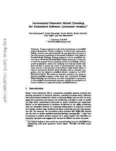
s2

s1

{p, q}

s3

{p}

Figure 2.1: Example of Kripke structure. Throughout this section, let AP be a finite set of atomic propositions ranged over by p, p0 , p1 , r, etc. As for propositional logic, atomic propositions are the most basic statements expressible in temporal logic. Definition 2.1.1 (Kripke structure). A Kripke structure is a tuple K = hS, I,→ − , Li where: • S is a countable set of states; • I ⊆ S is a set of initial states; •→ − ⊆ (S ×S) is a transition relation satisfying ∀s ∈ S.(∃s0 ∈ S.(s, s0 ) ∈ → −) • L : S → 2AP is an interpretation function on the set of state S, i.e., a function that assigns a set of atomic propositions to each state. In the following, we write s → − s0 as a shorthand for (s, s0 ) ∈ → − . The transition relation is total because of the condition imposed in the definition. Definition 2.1.2 (Path). Let K = hS, I,→ − , Li be a Kripke structure. A path in K is an infinite sequence of states s0 s1 s2 · · · such that si → − si+1 for all i > 0. As a convention for a path η = s0 s1 s2 · · · we write η[i] to denote the (i + 1)-th element and η i for the suffix of η starting at state i + 1, that is η i = si si+1 si+2 · · · . The set of paths starting at state s is defined by Path K (s) = {η ∈ S ω | η[0] = s, ∀i > 0 : η[i] → − η[i + 1]} . As a consequence of the condition imposed upon the transition relation of a Kripke structure K, we have Path K (s) 6= ∅ for any state s. Example 2.1.3. An example of Kripke structure is depicted in Figure 2.1. We have: S I

= {s1 , s2 , s3 } = {s1 }

→ − = {(s1 , s2 ), (s2 , s1 ), (s1 , s3 ), (s2 , s2 ), (s3 , s2 ), (s3 , s1 )} L = {(s1 , ∅), (s2 , {p, q}), (s3 , {p})}.

14

Chapter 2 – Preliminaries Definition 2.1.4 (Labelled Finite State Automaton). A labelled finitestate automaton (LFSA), over finite words, is a tuple A = hΣ, S,→ − , I, F, Li where • Σ is a finite alphabet; • S is a finite set of states; •→ − ⊆ S × S is a transition relation; • I ⊆ S is a set of initial states; • F ⊆ S is a set of accept states; • L : S → Σ is a function labelling the states. An equivalent and more widespread definition usually given, e.g., in compiler theory, labels transitions instead of states. Following [51, 71], here we prefer this definition since it suits better with the theory developed later on. As usual, for a finite alphabet Σ, let Σ∗ represent the set of all finite words and Σω the set of all infinite words, both over Σ. Definition 2.1.5. For a LFSA A = hΣ, S,→ − , I, F, Li, • a run ρ is a finite sequence of states ρ = s0 s1 · · · sn such that s0 ∈ I and si → − si+1 for 0 6 i < n. ρ is called accepting if sn ∈ F . • w = a0 a1 · · · an ∈ Σ∗ is an accepted word if there exists an accepting run ρ = s0 s1 · · · sn such that L(si ) = ai for all 0 6 i 6 n. • the language accepted is the set L(A) = {w ∈ Σ∗ | w is accepted by A}. LFSAs are often used to model the behaviour of terminating programs. Since, concurrent systems not always are supposed to terminate, their behaviour is modelled by finite automata accepting infinite words, called B¨ uchi automata [16]. B¨ uchi automata are defined as LFSA except for the definition of runs, which must be infinite. Definition 2.1.6. For a B¨ uchi automaton B = hΣ, S,→ − , I, F, Li, • a run ρ is an infinite sequence of states ρ = s0 s1 s2 · · · such that s0 ∈ I and si → − si+1 for i > 0. Let Inf (ρ) be the set of states occurring infinitely often in ρ. Then ρ is called accepting if Inf (ρ) ∩ F 6= ∅. • w = a0 a1 a2 · · · ∈ Σω is an accepted word if there exists an accepting run ρ = s0 s1 s2 · · · such that L(si ) = ai for all i > 0. • the language accepted is the set L(B) = {w ∈ Σω | w is accepted by B}. From this definition it follows that a run ρ is accepting if some accepting state occurs infinitely often.


15

There exist several kinds of B¨ uchi automata that are obtained by changing the notion of acceptance. An important one that we will use in the following, is the notion of generalised B¨ uchi automaton . In particular, a generalised B¨ uchi automaton has a set of sets of accept states of the form F ⊆ 2S (where S is the set of states). If F = {F0 , . . . , Fn }, a run of a generalised B¨ uchi automaton is accepting if Inf (ρ) ∩ Fi 6= ∅ ∀0 6 i 6 n (2.1) that is, for each set of accept states Fi , there is some state occurring infinitely often in ρ. It is interesting to note that the generalised acceptance condition does not extend the set of languages accepted by B¨ uchi automata. Kripke structures versus B¨ uchi automata. The two formal notion of Kripke structure and B¨ uchi automaton are closely related. In particular, a Kripke structure directly corresponds to a B¨ uchi automaton where all states are accepting and the alphabet is the power set of the atomic proposition. That is: let K = hS, I,→ uchi automaton is B = − , Li, then the corresponding B¨ h2AP , S,→ uchi automaton, can be seen as a Kripke − , I, S, Li. Vice-versa, a B¨ structure with a fairness condition determined by the set of accept states. In particular, a generalised B¨ uchi automaton is sometimes called in the literature fair Kripke structure [29]. Hence, every notion introduced in this chapter for Kripke structures can be restated in terms of B¨ uchi automata1 More on B¨ uchi automata. We now introduce some results on B¨ uchi automata that will be useful in Section 2.1.5. Given a B¨ uchi automaton B, there exists an automaton B such that L(B) = Σω \L(B)

(2.2)

i.e., B¨ uchi automata are closed under negation. For the rather involved construction of B, the reader is referred to [103]. B¨ uchi automata are also closed under intersection, that is given B1 and B2 there exists the automaton B1 ∩ B2 such that L(B1 ∩ B2 ) = L(B1 ) ∩ L(B2 ). (2.3) The construction of the intersection (or product) automaton is a modification of the definition of synchronous product of LFSA. The difficulty is given by the B¨ uchi acceptance condition that must be satisfied. B1 ∩ B2 can be constructed as follows. Let B1 = hΣ, S1 ,→ − 2 , I2 , F2 , L2 i then − 1 , I1 , F1 , L1 i and B2 = hΣ, S2 ,→ B1 ∩ B2 = hΣ, S,→ , I, F, Li where: − • S = {(s, s0 ) ∈ S1 × S2 | L1 (s1 ) = L2 (s2 )} × {1, 2} • I = (I1 × I2 ) × {1}) ∩ S 1 Being this chapter a overview on well established theories, when there will be the choice between Kripke structures and B¨ uchi automata we will try to follows what in the literature is more widespread.

16

Chapter 2 – Preliminaries • if s1 → − 1 s01 and s2 → − 2 s02 then (i) if s1 ∈ F1 then (s1 , s2 , 1) → − (s01 , s02 , 2) (ii) if s2 ∈ F2 then (s1 , s2 , 2) → − (s01 , s02 , 1) (iii) otherwise (s1 , s2 , i) → − (s01 , s02 , i) for i = 1, 2 • F = (F1 × S2 ) × {1}) ∩ S • L(s, s0 , i) = L1 (s). This construction was proposed in [23]. The automaton B1 ∩ B2 makes transitions when B1 and B2 perform steps on the same label. B1 ∩ B2 can be thought as having two tapes: states with third component 1 form the first tape whereas those with third component 2 form the second tape. The transition relation ensures that in order to visit infinitely many times the accept states in F , the accept states of both B1 and B2 must be visited infinitely many times as well. For the definition of F , it is enough to consider states in the tape 1 since by the transition relation the B1 ∩ B2 switches tape when visiting a state in F . Therefore, in order to visit a state in F again, the automaton must switch from tape 2 to tape 1. But, because of the definition of the transition relation this can happen only if the control of the automaton passes through an accept state of B2 . Thus, a run of B1 ∩ B2 traverses infinitely many times F precisely when both B1 and B2 traverse infinitely many times their set of accept states F1 and F2 . Note that setting F = F1 × F2 would not work since it requires not only that B1 and B2 visit accept states both infinitely often, but also that they do it at the same time ruling out, hence, some good runs.

2.1.2

Linear Temporal Logic In general there exists two main branches of temporal logics and their classification is based on the way time is modelled: linear time or branching time. For the interpretation of a formula, in the linear case every state may only have one successor state. On the contrary, in the branching case every state may have more than one. The main representative of the first kind is Linear Temporal Logic (LTL) introduced by Pnueli in 1977 [91]. Syntax of LTL. Let p ∈ AP be an atomic proposition. The syntax of Linear Temporal Logic is given by: φ ::= p | ¬φ | φ ∨ φ | Xφ | φ U φ. Intuitively, the meaning of the formulae is as follows: in a state ¬φ holds if φ does not hold; φ1 ∨ φ2 holds if either φ1 holds or φ2 holds; Xφ holds in a state if φ holds in the successive state. X is called next operator and represents the first temporal operator we encounter. Finally, φ1 U φ2 holds if φ2 eventually will


17

hold for some state and — until that state — φ1 continuously holds. U is called until operator. From this basic syntactic definition of LTL, it is customary to define other connectives as syntactic sugar: tt ff φ∧ψ φ⇒ψ φ⇔ψ Fφ Gφ

≡ ≡ ≡ ≡ ≡ ≡ ≡

p ∨ ¬p ¬tt ¬(¬φ ∨ ¬ψ) ¬φ ∨ ψ (φ ⇒ ψ) ∧ (ψ ⇒ φ) tt U φ ¬F(¬φ)

[eventually φ] [globally φ]

Most of these abbreviations are standard in propositional logic, the last two are typical of LTL. Intuitively, Fφ means that either φ is true now or it will become true in some state in the future. Gφ means that φ holds in the current state and it holds in every state in the future. Semantics of LTL. The term linear in LTL derives from the fact that formulae are interpreted over sequences of states representing computation of a system modelled by a Kripke structure K = hS, I,→ − , Li. These sequences are paths of K. Let p ∈ AP be an atomic proposition, η a path and φ, ψ be LTL formulae. The satisfaction relation |= is given by: η |= p η |= ¬φ

iff p ∈ L(η[0]) iff not (η |= φ)

η |= φ ∨ ψ η |= Xφ

iff either (η |= φ) or (η |= ψ) iff η 1 |= φ

η |= φUψ

iff ∃j > 0 : η j |= ψ ∧ (∀0 6 k < j : η k |= φ))

As for propositional logic, an atomic proposition p is true in a state η[0] if it is among the interpretations given by L(η[0]). A negated formula ¬φ is valid in a state if φ is not valid in the same state. The disjunction φ ∨ ψ is valid when at least one of φ, or ψ is valid in the same state. The next operator is more interesting since it is proper of temporal logics. Xφ is satisfied by a path η if the formula φ is valid in the path starting from the successor state of η[0]. Finally, the until formula φ U ψ is satisfied if ψ become valid on a path starting at η[0] or starting from a state following η[0], say η[j] with j > 0 . Furthermore, it is required that in every path starting with a state between η[0] and the predecessor of η[j], the formula φ is continuously valid.

2.1.3

Computation Tree Logic For the sake of completeness, we give some notions of branching temporal logic. Although in the remaining of the thesis we will focus on linear temporal logics,

18

Chapter 2 – Preliminaries the present overview may help the reader to realise that several of the definition introduced in the following chapters in a linear setting can be restated, and therefore applied, in a branching temporal logic. Computation Tree Logic (CTL), introduced by Clarke and Emerson in 1981 [26], is a temporal logic that has a branching notion of time (in contrast with LTL), i.e, for every state there can be more that one possible successor state. The underlying notion of semantics of a branching temporal logic is a tree of states rather than a sequence. Like a sequence, a tree is obtained from a Kripke structure by a process of “unfolding”. The outgoing transitions starting from a state represent the possible next states, and CTL allows to reason about all or some of the paths by a special quantifier over paths. Syntax of CTL. As usual let AP be a set of atomic propositions ranged over by p, q, r. The syntax of CTL is defined by the following grammar: φ

::= p | ¬φ | φ ∨ φ | EXφ | E[φ U φ] | A[φ U φ].

The temporal operators have the following intuitive meaning: • EXφ expresses that there is a next state in which the formula φ holds. • E[φUψ] expresses that there exists a path starting from the current state along which ψ holds at a given state, and φ holds in every state before. • A[φUψ] expresses that along every path starting from the current state, ψ holds at a given state and φ holds in every state before. As usual, by combining these basic operators we can obtain other auxiliary operators. The first two correspond to the case where the first formula is tt. We have: EFφ ≡ E[tt U φ] [potentially φ] AFφ ≡ A[tt U φ] [φ is inevitable]. Finally, by negation we erators: AXφ AGφ EGφ

can define the (very useful) duals of the previous op≡ ¬EX¬φ ≡ ¬EF¬φ ≡ ¬AF¬φ

[for all path next φ] [invariantly φ] [potentially always φ].

Given a state s the previous connectives have the following intuitive meaning. EFφ is valid in s if and only if eventually φ holds along at least one of the paths starting at s, whereas AFφ is valid in s if and only if φ holds in all paths starting at s. The formula EGφ holds in s if there exists some path starting at s where φ holds along every state of this path. Symmetrically, AGφ holds in s if and only if φ holds in every state of every path starting at s.


19

Semantics of CTL. Also the semantics of CTL is based on the notion of Kripke structure. Given a Kripke structure K = hS, I,→ − , Li and state s ∈ S, there exists a infinite computation tree rooted at s such that (s0 , s00 ) is an arc of the tree if and only if s0 → − s00 and s0 is reachable from s. The semantics of CTL is defined by satisfaction relation |= between the Kripke structure K, a state s and a formula φ. We write K, s |= φ if and only if φ holds in the state s of K. The structure K is usually omitted if it is clear from the context. Let p ∈ AP be an atomic proposition, K = hS, I,→ − , Li be a Kripke structure, s ∈ S, and φ a CTL formula. The satisfaction relation |= is defined by: s |= p

iff p ∈ L(s)

s |= ¬φ s |= φ ∨ ψ

iff not (s |= φ) iff either (s |= φ) or (s |= ψ)

s |= EXφ s |= E[φUψ]

iff ∃η ∈ Path K (s) : η[1] |= φ iff ∃η ∈ Path K (s) : (∃j > 0 : η[j] |= ψ ∧ (∀0 6 k < j : η[k] |= φ))

s |= A[φUψ]

iff ∀η ∈ Path K (s) : (∃j > 0 : η[j] |= ψ ∧ (∀0 6 k < j : η[k] |= φ)).

The interpretation of atomic propositions, negation, disjunction is the same as for LTL. EXφ is true if there exists a path among those starting at s that satisfies φ in the next state. The interpretation of A[φ U ψ] and E[φ U ψ] is the same as φ U ψ in LTL, except that there is the existential and the universal quantification on the paths starting at s. Namely, we require that the until formula holds for at least one path in E[φ U ψ] and for every path in A[φ U ψ].

2.1.4

A few formal notions relating formulae and models Given a Kripke structure K modelling the behaviour of a system and a formula φ expressed in some temporal logic, e.g., LTL or CTL, representing a specification of the system, we have several notions relating K and φ. We give the definition for the case of LTL. Definition 2.1.7. Let K = hS,→ − , I, Li be a Kripke structure and φ a LTL formula: K |= φ iff ∀s ∈ I : (∀η ∈ Path K (s) : η |= φ) When K |= φ we say that K satisfies φ. The notion of satisfiability given by Definition 2.1.7 corresponds to the informal idea that an implementation satisfies a specification, that is: if no possible computation of the system does violates the specification given by φ. Definition 2.1.7 takes origin in logic from the well-known satisfiability problem (SAT) defined in Table 2.1. For propositional LTL, (SAT) is decidable, but for other logics it is not (e.g., first-order logic). Indeed this is a rather hard problem since only φ is given whereas K must be somehow determined and/or constructed.

20

Chapter 2 – Preliminaries Dual to the satisfiability problem is the validity problem (VAL) again defined in Table 2.1. To decide (VAL) for φ, one can solve the the satisfiability problem for ¬φ since if a formula is valid then its negation is unsatisfiable. The third problem defined in Table 2.1 is the model checking problem (MC). In that case, the Kripke structure K is given and we must “only” verify that it satisfies φ. The model checking problem conforms more to the idea of software verification, since it essentially tries to verify whether a model of an implementation (i.e., K) satisfies a specification (i.e., φ). In contrast, an algorithm showing (SAT) can be used as a feasibility test for a specification φ: in fact, if φ does not pass the test it cannot be implemented at all, therefore another specification must be provided. In this thesis, we deal with issues related to (MC). Hence, every time, we consider the case where K is given. We can see K in two different ways [99]: • as a post-design or pre-implementation model; in this case K is used to verify the design of a system and it can help to define a candidate implementation that is supposed to satisfy the specification φ. This point of view corresponds to the “classical” model checking approach. • as post-implementation model; in this case K is used as a verification model of an existing implementation and the aim is the debugging of the implementation. This point of view corresponds to the “modern” model checking approach (cf. Section 1.1 for related issues). Along the lines of the two previous points of view, we refine the notion of satisfiability and validity given above in order to be more related to the idea of computations performed by K. In fact, because of the two universal quantifications, Definition 2.1.7 has more the flavour of validity in terms of the computations performed by K. The last two problems defined in Table 2.1 are parametric (dependent) on K. The K-validity problem (K-VAL) corresponds to (MC), although the quantification (and therefore the emphasis) is on the computation rather than on the model K. The dual problem of (K-VAL), is the K-satisfiability problem (K-SAT). (K-SAT) asks if there exists (at least) one computation in K satisfying φ whereas (K-VAL) asks if every computation of K satisfies φ. Again the difference between (SAT), (VAL), (K-SAT) and (K-VAL) is that the quantification in the former two is on the Kripke structure K whereas in the latter two the quantification is over the computations of a given K. Note that solving (K-VAL) corresponds to solving (MC) and by solving (KSAT) for ¬φ we automatically determine an answer for (K-VAL). Moreover, the corresponding notions of (K-VAL) and (K-SAT) for B¨ uchi automata will be introduced in Chapters 4 and 5 for the special case of HABAs which are the automata we are going to define and use there.

2.1.5

The automata theoretic approach to model checking Automata, and in particular B¨ uchi automata, can be used not only to describe the behaviour of concurrent systems but also to formalise the specifications of


21

(SAT)

given a formula φ, does there exist a Kripke structure K such that K |= φ?

(VAL)

given a formula φ, is it K |= φ for every Kripke structure K?

(MC)

given a formula φ and a Kripke structure K, is it K |= φ?

(K-VAL)

given a formula φ, is it ∀s ∈ I : (∀η ∈ Path K (s) : η |= φ)?

(K-SAT)

given a formula φ, does there exists a s ∈ I such that there exists η ∈ Path K (s) such that η |= φ?

Table 2.1: Definition of satisfiability, validity and model checking problem. the systems. The advantage of using specifications by automata is that both the system and the specification are described with the same formalism. Let Bspec be a B¨ uchi automaton describing the specification of a system. Then its language L(Bspec ) is the set of allowed behaviours for the system. Let Bsys be the B¨ uchi automaton modelling the system. The system satisfies its specification Bspec if L(Bsys ) ⊆ L(Bspec ). (2.4) Stated in words, this set inclusion says that the set of behaviours of the system are among those behaviours allowed by the specification. We can restate (2.4) using the automaton Bspec accepting the complement of the language L(Bspec ) (see Section 2.1.1) in the following way: L(Bsys ) ∩ L(Bspec ) = ∅.

(2.5)

If this intersection would not be empty, any infinite word contained would represent a counterexample. From (2.5) we can derive in a straightforward manner the model checking Algorithm 1 (reported in pseudo-code). Algorithm 1 Automata theoretic procedure for model checking 1: procedure ModelChecking(Bspec , Bsys ) do 2: Construct the automaton Bspec ; 3: Construct the automaton Bsys ∩ Bspec ; 4: if L(Bsys ∩ Bspec ) = ∅ then 5: Output:“The system satisfies the specification”; 6: else 7: return as a counterexample a word in L(Bsys ∩ Bspec ); 8: end if 9: end procedure ModelChecking In many cases, the specification is not directly expressed in terms of automata but by a specification language such as LTL. There exists a method

22

Chapter 2 – Preliminaries that automatically translates an LTL formula φ into an automaton, say Bφ , that accepts precisely the runs satisfying φ [51]. In this method, Bspec (of Algorithm 1) is represented by Bφ . It is interesting to note that when Bspec is obtained by the translation of a LTL formula φ, the construction of the complemented automaton (cf. step 1) can be skipped by constructing directly the automaton describing ¬φ, i.e., B¬φ . We have seen in Section 2.1.1 how the construction of the automaton Bsys ∩ Bspec can be done. The condition L(Bsys ∩ Bspec ) = ∅ is not straightforward and therefore deserves some further explanation. Checking for emptiness. Since an accepting run ρ of a B¨ uchi automaton B = hΣ, S, →, I, F, Li contains infinitely many occurrences of accept states and S is finite then there must exist ρ0 and ρ00 such that ρ = ρ0 ρ00 and all the states in ρ00 appear infinitely many times. Hence, states in ρ00 must be contained in a strongly connected component (SCC), say Sρ00 . Furthermore, since ρ is a run, it follows that: (a) Sρ00 is reachable from an initial state; (b) Sρ00 ∩ F 6= ∅. Conversely, to any SCC for which (a) and (b) holds, a corresponding accepting run of B does exist. This suggests that in order to verify that the language is not empty, we can check for the existence of a SCC reachable from an initial state and containing at least an accepting state. Finding such a SCC boils down to finding a cycle containing some accepting state. In fact, if there exists a SCC then this must be contained in a cycle, conversely, if there exists a cycle, it must correspond to a SCC. The implication of this observation is that it is possible to represent a run of a B¨ uchi automaton in a finite way. This is particularly interesting for runs of Bsys ∩ Bspec , since they correspond to computations in which the system does not satisfy the specification, i.e., counterexamples. Summarising, two steps must be done: 1. find the set Freach of all accept states reachable from an initial state; 2. find a cycle containing some state s ∈ Freach . The construction of Freach can be done in linear time by a depth-first search. Step 2, which amounts to detecting cycles in a finite graph, can also be done in linear time using Tarjan’s algorithm [107] for constructing SCCs in a graph. The complete procedure for step 1 and 2 will have a time complexity of O(|S|+ |→|). A slightly better solution is the Algorithm 2 known as nested depth-first search and proposed in [35]. It detects reachable accept states and cycles containing them at the same time. The advantage of this last solution is that the search can be done on-the-fly. In particular, errors are detected while traversing the state space and the procedure can be stopped as soon as the first error is caught. The procedure NestedDFS can be explained as follows.


23

Algorithm 2 Nested depth-first search 1: procedure NestedDFS(B) do 2: for all s ∈ IB do 3: DFS1(s); 4: end for 5: return []; 6: end procedure NestedDFS 7: 8: 9: 10: 11: 12: 13: 14: 15: 16: 17: 18:

procedure DFS1(s) do Insert s in Stk1 ; for all s0 such that s → s0 do if s0 ∈ / Stk1 then DFS1(s0 ); end if end for if s ∈ FB then DFS2(s); end if end procedure DFS1

19: 20: 21: 22: 23: 24: 25: 26: 27: 28: 29:

procedure DFS2(s) do Insert s in Stk2 ; for all s0 such that s → s0 do if s0 ∈ Stk1 then return counterexample; else if s0 ∈ / Stk2 then DFS2(s0 ); end if end for end procedure DFS2

It calls for every initial state the procedure DFS1 that, in turn, traverses in depth-first manner the graph, putting every visited state in the stack Stk1 till it has to backtrack on an accept state. Then, DFS1 calls DFS2 which is in charge of finding out if the current accept state s is contained in a cycle. Again, DFS2 explores the state space in depth-first manner till it finds a successor of the accept state, say s0 , that has been already visited by DFS1, i.e., s0 ∈ Stk1 . If this is the case, a cycle has been found and the procedure terminates successfully. The counterexample is given by the sequence of states in the stack Stk1 up to s that constitutes the prefix of the SCC. Finally, the SCC itself is constructed by taking the states in Stk2 that form a path from s to s0 and closing the cycle with the states in Stk1 that form a path from s0 to s.

24

2.1.6

Chapter 2 – Preliminaries

The tableau approach to model checking An alternative algorithm for model checking LTL is based on the construction of a tableau graph. This method was introduced by Lichtenstein and Pnueli in [77]. In general, the construction of the tableau graph depends on the formula φ we want to model check and on the Kripke structure K. The main property of the tableau graph is the following: a model for the formula φ can be extracted from it if and only if the formula is satisfiable in K. Moreover, another important property of the tableau is that it is a finite structure which embeds all possible models of the formula. We briefly summarise the construction of the tableau graph for the formula φ and the Kripke structure K. The closure of φ, denoted by CL(φ), is the set of formulae whose truth value may influence the truth value of φ itself. Definition 2.1.8. Let φ be an formula. The closure of φ, CL(φ), is the smallest set of formulae (identifying ¬¬ψ with ψ) such that: • φ, tt, ff ∈ CL(φ); • ¬ψ ∈ CL(φ) iff ψ ∈ CL(φ); • if ψ1 ∨ ψ2 ∈ CL(φ) then ψ1 , ψ2 ∈ CL(φ); • if Xψ ∈ CL(φ) then ψ ∈ CL(φ); • if ¬Xψ ∈ CL(φ) then X¬ψ ∈ CL(φ); • if ψ1 U ψ2 ∈ CL(φ) then ψ1 , ψ2 , X(ψ1 U ψ2 ) ∈ CL(φ). The tableau graph for K and φ denoted by GK (φ) is given by a set of vertexes AK (φ) and a set of arcs → ⊆ AK (φ) × AK (φ). The vertexes of the tableau, called atoms, are composed by states of K decorated with a maximal set of consistent formulae compatible with the labelling of K, i.e. the interpretation function L. Definition 2.1.9. Given a Kripke structure K = hS, I, →, Li, and a formula φ, an atom is a pair A = (s, D) with s ∈ S and D ⊆ CL(φ) ∪ AP such that: • if p ∈ AP , then p ∈ D iff p ∈ L(s); • if ψ ∈ CL(φ), then ψ ∈ D iff ¬ψ ∈ / D; • if ψ1 ∨ ψ2 ∈ CL(φ) then ψ1 ∨ ψ2 ∈ D iff ψi ∈ D for i = 1 or i = 2; • if ¬Xψ ∈ CL(φ), then ¬Xψ ∈ D iff X¬ψ ∈ D; • if ψ1 U ψ2 ∈ CL(φ), then ψ1 U ψ2 ∈ D iff either ψ2 ∈ D, or both ψ1 ∈ D and X(ψ1 U ψ2 ) ∈ D.


25

We denote the first and the second components of an atom A = (s, D) by sA and DA , respectively. To complete the construction of the graph GK (φ), we must define arcs between vertexes. Those take into account the semantics of the formulae contained in the atoms and the transitions of the Kripke structure. Definition 2.1.10. The tableau graph GK (φ) for K and φ consists of vertexes AK (φ) and arcs → − ⊆ AK (φ) × AK (φ) determined by: s → s0 and 0 0 (s, D) → (s , D ) ⇔ ∀Xψ ∈ CL(φ), (Xψ ∈ D ⇔ ψ ∈ D 0 ) Hence the resulting graph will mimic the behaviour of K as long as the formulae involving temporal operators are satisfied. For the definition of the arcs, it is sufficient to require the consistency of the next operator X. A path π of GK (φ) is an infinite sequence of atoms π = A0 A1 A2 · · · in G such that • s Ai → − sAi+1 for all i ≥ 0; • if ψ1 U ψ2 ∈ DAi for some atom i ≥ 0, then there exists an atom Aj with j ≥ i such that ψ2 ∈ DAj . Thus a path2 corresponds to a run of K and while ensuring the satisfaction of until formulae. Let σ = sA0 sA1 sA2 · · · , the path π fulfils φ if σ |= φ. The presence of a formula in an atom Ai belonging to a fulfilling path π is related to the satisfaction of that formula in the model underling the path from state i on, i.e., π i . More precisely we have the following fact whose proof is given in [77]. Proposition 2.1.11 (Lichtenstein and Pnueli [77]). • π = A0 A1 A2 · · · fulfils φ if and only if φ ∈ DA0 . • φ is satisfiable if and only if there exists a path π fulfilling it. By the previous proposition we can conclude that in order to check the satisfiability of a formula φ in K it is sufficient to look for a fulfilling path in the tableau GK (φ). However, in a graph there may be infinitely many different paths, therefore Proposition 2.1.11 still does not provide us with a computable method. A strongly connected subgraph (SCS) G0 ⊆ GK (φ) is called self-fulfilling if for every A ∈ G0 such that ψ1 U ψ2 ∈ A there exists B ∈ G0 such that ψ2 ∈ DB . Let Inf (π) denote the set of atoms that appear infinitely often in the path π. 2 By some unfortunate coincidence, the term “path” is used for two different mathematical objects, i.e., a sequence of states in a Kripke structure and a sequence of atoms in the tableau graph. In the following we will specify which object we are referring to, unless it is clear from the context.

26

Chapter 2 – Preliminaries Proposition 2.1.12 (Lichtenstein and Pnueli [77]). • If π is fulfilling then Inf (π) is a self-fulfilling SCS of GK (φ). • for every self-fulfilling SCS G0 ⊆ GK (φ) there exists a fulfilling path π such that Inf (π) = G0 . An immediate consequence of this proposition is that φ is satisfiable if and only if there exists an initial atom A in GK (φ) such that φ ∈ DA and a selffulfilling SCS is reachable from A. Indeed this proposition can be used to define a mechanical way to verify the satisfaction of the formula φ since there are only a finite number of SCS in GK (φ). The algorithm presented in this section has a complexity linear in the size of K and exponential in the size of φ (cf. [77]).

2.1.7

Automata theoretic versus tableau approach After having summarised the automata theoretic approach in Section 2.1.5 and the tableau method in Section 2.1.6, it is natural to ask which method is more suitable for our study. The argument in favour of the automata-theoretic approach is essentially that it can be performed on-the-fly [51] meaning that it is not necessary to construct the complete state space of the B¨ uchi automaton Bsys modelling the system. Instead, states of Bsys are generated only when it is needed during the construction of the product automaton. This means that it is not always necessary to construct the complete Bsys since we can find a counterexample before, and thus we can stop the procedure at that point. As a direct consequence, the automata theoretic method may help to alleviate the problem of state-space explosion. This occurs when in order to model the system accurately, the automaton Bsys needs a number of states that is too large (normally exponential in the number of components of the system) and exceeds the computer memory. Currently this is the main problem of model checking. In contrast, in order to apply the tableau method described in Section 2.1.6 we need the complete Kripke structure modelling the system which (again) can be rather large. Of course, the automata-theoretic approach (for LTL) relies on the feasibility of the construction of the B¨ uchi automaton corresponding to the negation of the LTL formula we want to verify. However, if we change focus, and from LTL we move to some other specification language, the situation may be different. And in fact, this is what happens, for example, with the logic A``TL that we study in Chapter 4. For this logic, the construction of the automaton for a given formula is most likely undecidable3 due to the very dynamic nature of its models. Being able to construct the automaton for every formula of the logic corresponds to solve the satisfiability problem (SAT), although we are mainly interested in the model checking problem (MC) (cf. Section 2.1.7). 3 The study we have carried out in the past strongly suggest the undecidability of the problem, although we do not have any proof of this conjecture.

2.2 History-Dependent Automata

27

This consideration has led us to consider the tableau method. In that approach, the only Kripke structure involved is the one corresponding to the behaviour of system (that is given). Furthermore, this given Kripke structure guides us in the construction of the tableau graph. Hence, in this sense, the method appears to be more promising, since somehow, it overcomes the construction of the automaton corresponding to the formula. In the subsequent chapters we will use the tableau method and see that it can be effectively exploited to develop model-checking algorithms for logics with a high degree of dynamism such as A``TL.

2.2

History-Dependent Automata History-dependent formalisms are those whose actions performed in a particular state may depend on actions performed in previous states. A typical history-dependent formalism is the π-calculus [82] where, for example, channel names are created in some state and can be referred to in some other successive state. Other history-dependent formalisms are CCS with localities [11] and Petri Nets. In general, the semantics of history-dependent formalisms is given in terms of labelled transition systems. Ordinary automata, such as LFSA given by Definition 2.1.4, present some limitations in dealing with such kinds of calculi. Even very simple actions may produce infinite state spaces. This is clearly problematic for the application of formal techniques such as model checking which, as we have seen, mostly require the inspection of a finite-state model. Montanari and Pistore introduced an extension of ordinary automata, called History-dependent (HD) automata [83, 84, 90] that are meant to represent adequate models for history-dependent formalisms, overcoming therefore the limitations of LFSA. Notice that object-based systems have a clear history-dependent behaviour since, for example, objects are created and can be referenced to in the future. Therefore, the features of HD-automata can be exploited to model the birth and death behaviour of objects. We quickly introduce a (specialisation of the) definition of HD-automata that differs slightly from the original definition of HD-automaton given in [84] but easier fits towards our needs4 . Let N be a countable set of global names. Definition 2.2.1. A HD-automaton A is a tuple hQ, N,→ − , q0 i where: • Q is a (possibly infinite) set of states; • N : Q → 2N is a function that associates to each state q ∈ Q a finite set Nq of names; •→ − ⊆ Q × (N * N) × Q, such that for q → − λ q 0 , we have λ : Nq * Nq0 injective; 4 This is only done for the sake of simplicity in the presentation since the definitions of our formalisms (cf. Chapters 4 and 5) resemble the one given here.

28


s a c

b

s0 g d

e

f

Figure 2.2: A simple HD-automaton. • q0 ∈ Q is an initial state; States of an HD-automaton are equipped with a set of local names that can be created dynamically. The transitions are equipped by a partial injective mapping λ from names of the source state to names of the target state. Since names do not have a global identity, a single state of an HD-automaton can be seen as an abstraction of the set of all states that differ only by bijective re-namings of names. The correspondence between the local names of two successive states is ensured by the mapping λ attached to the transitions. The difference between Definition 2.2.1 and the original definition of HDautomaton given in [84] is essentially that in the latter, not only states are equipped with names but also transitions and labels (in the transitions). The correspondence between names of the source state with the those of the target state is split in two mappings (instead of one like in Definition 2.2.1): the first mapping goes from the names of the source state to the names of the transitions and second mapping from the name of the target state to the names of the transition. We will not further consider the difference between Definition 2.2.1 and that given in [84]. Names appearing in a state (of an HD-automaton) are considered to be currently in use, i.e., alive. The mapping attached to the transition is partial, giving the possibility to distinguish three categories of names: (i) names that are mapped from the source to the target state are preserved in the transition; (ii) names that appear in the source state but not in the target state are deallocated; (iii) names that appear only in the target state are created. Example 2.2.2. A simple HD-automaton is shown in Figure 2.2. We have Q = {s, s0 }; the initial state (q0 in the definition) is s. Names are depicted by small circles, therefore we have: N (s) = {a, b, c}, N (s0 ) = {d, e, f, g}. The mapping λ is represented by dashed lines. By of λ, b is deallocated when the transition is fired, whereas the name a in s is renamed into g in s0 and c is renamed into f . It is important to stress the local nature of names, in fact if we assume that a represents a name of an object, then the same object after the transition is called g. Names d and e are new in s0 .

2.3 Object-based systems

29

The local nature of names in HD-automata is helpful because the states can be identified up to renaming, i.e., the actual identity of names does not matter. This is beneficial when it comes to give the semantics to history-dependent formalisms such as the π-calculus. Without entering in the details (for which we refer the interested reader to [84]), it is enough to mention that the semantics of π is usually given in terms of standard labelled-transition systems. Furthermore, in the π-calculus, an agent in every state uses a certain set of names. Also, there exists an input action in which the agent receives a name via a channel that is bound to a variable, say x. However, an input action generates a infinite number of transitions because x can be bounded with any possible name in N not used by the agent (and there are infinitely many of such names). Thus, even a really simple agent (with only an input action) may generate an infinite transition system. The important point there is that it does not matter which name is bound to x, every choice is equivalent, but this fact is not exploited in a standard transition systems semantics. With local names instead, since we can identify states up to renaming of names, the infinite branching transitions can be collapsed into a single one by, for example, choosing a representative name to bind to x. Another advantage is that it is possible to obtain a minimal automaton up to bisimulation. Finally, it is interesting to note that a large class of finitary π-calculus agents5 correspond to finite-state HD-automata that in turn can be translated into finite ordinary automata, in such a way that bisimilar HD-automata correspond to bisimilar ordinary automata. Dealing with the latter is convenient since standard algorithms may be applied. In Section 2.3.2, we will see that object-based systems are highly dynamic also because of the allocation and deallocation of objects. Here we have learnt that HD-automata are a formalism suited to model (in a compact way) the allocation and deallocation of names. In studying models oriented towards the verification of dynamic properties of object-based systems it therefore becomes natural to look at HD-automata as a starting point. Indeed, in Chapter 4 and 5 we will define two classes of B¨ uchi automata — very much inspired by HD-automata — that also exploit the advantage of having local names and remapping in order to obtain more compact models.

2.3

Object-based systems In this thesis, we confine ourselves to object-based systems, i.e., object-oriented systems in which inheritance and sub-typing are not considered 6 . Object-based systems are composed by objects that run concurrently and communicate with 5 For the reader familiar with the π-calculus, finitary agents are those where parallel composition does not occur in the bodies of their recursive definitions. 6 In other classifications (e.g. [1]), object-based languages do not have classes in contrast to class-based languages. We will not use this classification.

30

Chapter 2 – Preliminaries each other. Objects are dynamic, can be created in arbitrary number and can be deallocated during the computation. Objects. At the conceptual level, an object can be seen as an entity that has an identity, a state and a behaviour. This definition has originally been given by Booch [8]. The state of the object contains internal data that can only be accessed from the outside by invoking one of the object’s methods. The invocation is done by sending a message to the object. Data are usually called attributes and they have a value of a certain type. Depending on the definition of the object, some attributes may be modified while others may not. The behaviour of the object is the reaction that the object has after having been stimulated by a message from the outside world. The way an object behaves is in general dependent from its current internal state. The outside world is constituted by other objects running concurrently. The identity of the object is distinct from its state: the value of its attributes may change during the computation although the object’s identity remains fixed. In general an object is created at a certain point in time, and it may die successively. However, between the moment in which the object is born until it dies, the object is continuously alive and is identified by its identity. In later chapters in this thesis we will deeply investigate the nature of object identity. In our models, we will clearly distinguish between the identity of an object and its state. We will also give identity to a method invocation. A justification will become clear later. Classes. On the static level, the corresponding notion of object is that of a class. A class is a template for the creation of its instances, i.e., its objects. A class specifies the state of its objects by describing the attribute types, and the objects behaviour by the definition of a set of methods. A method is a fragment of code that implements an operation. The implementation is hidden, the only thing the outside world knows is that the objects belonging to the class provide that operation. Methods of a class are executed by instances of the same class. The set of class operations that can be invoked from the outside is known as the interface of the class. Interfaces are useful to increase the abstraction of the classes since methods and attributes not included in any interface are hidden to the outside7 . We refer to the object executing a method as the owner of the method. A special keyword that may be used in the code of the method is self. At run-time, it refers to the identity of the owner8 . By self a method can access the attributes (i.e., the state) of its owner. 7 Here we use the term “abstraction” in a different way than the rest of the thesis, where in general abstraction will describe some technique to reduce the state space of a model. 8 Some languages such as Java of C++ prefer the notation this instead of self.


2.3.1

31

The Unified Modelling Language The Unified Modelling Language (UML) [9, 98] is the standard modelling languages accepted by the Object Management Group (OMG) in 1997. It is the result of a merging process of different notations previously existing. The UML provides the designer with several types of diagrams that concentrate on a special part of the system, amongst others: • the use case diagram concentrates on the interaction between the user of the system (called actors) and the system itself; • the class diagram focuses on the relation between classes of the system. • the sequence diagram describes the behaviour of the system by showing the interaction of objects through the messages they interchange. • the object diagram models a single state (of a computation) of the system (sometimes called snapshot). It contains the values of the object attributes as well as the references between objects; the latter take the form of links among them. • the state chart diagram describes the life cycle of an object by a sequence of states of a state machine associated with the object. Since in this thesis we will be concerned only with class diagrams, we introduce some of their basic concepts. Class diagrams. In UML, the static structure of classes in the system and their associations are described by class diagrams that illustrate for each class • the attributes with their type, and • the methods with their formal parameters. A simple example class diagram (adopted from [111]) is depicted in Figure 2.3, Boxes represent classes. Three parts, delineated by a line, can be distinguished in a box. The class name is indicated in the upper part, thus in our system we have three classes: Hotel, Room, and Guest. The attributes of the class together with their types are reported in the middle part of the box. For example, the class Hotel has only two attributes numOfFloors and numOfRooms, whereas both Room and Guest have three attributes. The attribute name is followed by the attribute type (separated by a colon sign ‘:’). In the example, both numOfFloors and numOfRooms have type Integer. Finally, the bottom part of a box lists the operations (or methods) of the class. The signature of an operation describes its name, its formal parameters and the return type (if any). The formal parameters are depicted between parentheses indicating also their type. Thus for example, the class Hotel has two operations checkIn and checkOut, respectively, with only one parameter of type Guest and without return type. Classes Room and Guest do not have any operation.

32

Chapter 2 – Preliminaries Boxes are interconnected by lines denoting associations. They represent the relationship between classes. Each direction of an association has an optional name (called role name) and multiplicity giving information on the number of elements related by the association. For instance, the multiplicity 1..∗ states that a Hotel has at least one room, whereas on the association relating Hotel and Guest, ∗ says that the Hotel can have a number of guests greater or equal to zero (i.e., the hotel can be empty). If the multiplicity is not specified it is intended to be one. Note that class diagrams only address the static aspects of the system, not its dynamic (i.e., process) aspects. The latter aspects are described by other diagrams such as UML state-charts. Navigation. An important factor is that associations between classes in UML diagrams can be traversed. Thus, they constitute a path within the model that allows to reach a class starting from another class. This phenomenon is referred to as navigation (or navigability) and allows to refer to attributes and methods of a (collection of) object(s) in the system. As we will see in Section 3.4, in the notation used by the Object Constraint Language [110], navigations are expressed by indicating the role name attached to the association we want to traverse. For instance, for an object of class Hotel denoted by the variable h, the expression h.guests refers to the path between class Hotel to the class Guest using the association with role name guests. Navigations are parsed from left to right. The navigation expression h.guests.guestCode refers to the collection of guests’ code of h.

2.3.2

Dynamic allocation and deallocation Concurrent object-based systems are characterised by a highly dynamic behaviour. A first interesting source for this dynamic behaviour comes from the lives of objects. During the computation, objects are created by some creation mechanism provided by the programming language that must be invoked explicitly. For example, for the Hotel example in Java we would write new Hotel() to create an instance of the class Hotel. Here, Hotel() represents a constructor, that is, a procedure specifying in detail how to build the object and how to initialise its attributes. Several constructors can be defined for the same class according to different possibilities and/or needs to create objects. Moreover, during the computation some object may die either because of an explicit command given by the programmer (such as delete in C++) or because of some system routine (e.g. garbage collection). In any case, an object-based computation does not have a static pre-allocated number of objects that will remain fixed till the end. This model of computation is therefore different from the more traditional programming languages (e.g. Pascal or C)


33

Room

Hotel

floorNumber : Integer rooms 1..* roomNumber : Integer numOfBeds : Integer

numOfFloors : Integer hotel

numOfRooms : Integer

0..1 room

checkIn(g : Guest) checkOut (g : Guest) 0..1 hotel

* guests

Guest

guests *

guestCode : Integer age : Integer numOfNights : Integer

Figure 2.3: The Hotel class diagram. where most of the resources are allocated statically according to the declarations contained in the program. Figure 2.4 depicts a sequence of three run-time states of an object-based system. The internal structure — that sometimes will be referred to as (object-) heap — shows the alive objects (and their references). In the state s1 , six objects are alive: o1 through o6 . In the successor state s2 , the object o5 has died, whereas o7 , o8 have been created. Finally, in state s3 , object o1 dies. We can paraphrase the previous description moving the focus towards the lives of the single heap-allocated objects9 as follows: In state s1 , the objects o1 , o2 , o3 , o4 , o5 , o6 are alive. In state s2 object o5 is dead and o1 , o2 , o3 , o4 , o6 , o7 , o8 are alive, from which o7 and o8 are new (i.e., fresh) whereas o1 , o2 , o3 , o4 , o6 are old. In state s3 the object o1 is dead and o2 , o3 , o4 , o6 , o7 , o8 are alive and at the same time old. This second description gives us an important hint: the substantial properties that allow us to capture the dynamism of the system w.r.t. the lives of objects are given by the following four adjectives: new, old, alive, dead. This will be used later on. Furthermore, it is clear that “old” is synonym of alive but nonnew as well as “dead” is synonym of non-alive, therefore in principle we can focus on only two of this object status10 . 9 This

is essentially the dynamic evolution of the system we want to capture of course, that we can use an operator expressing negation.

10 Provided,

34


o5

o1

s1

o3

o4

o2 o6

o3

o1

s2

o4

o2 o8

o7

o6

o3

s3

o4

o2 o7

o8

o6

Figure 2.4: Sequence of states in a concurrent object-based system. The models that we aim to develop must be as general as possible. In principle, there is no reason to admit in our models only objects that are created during the computation and that will die at some point in the future. In the history of the humanity many models have been developed where entities were supposed to have been always alive, or that would not die. It is enough to think about the several religions or ancient mythology. Thus — beside (standard) objects that are born in some state of the computation and die in some other state — we can very well have immortal objects that do not die at all during the computation (cf. Java real-time); or eternal objects that are alive but they are neither born nor die in any state of the computation. Modelling the states of an object-based computation as described in Figure 2.4 is quite expressive and general. Unfortunately, the model becomes somehow naively idyllic once we try to apply it for model-checking technology. There are two problems related to the object model presented above. First of all, as we have previously remarked, the model-checking motto is brute force: the state-space must be completely covered in order to fully apply this technique. Secondly, computer memory is finite. As a consequence, we cannot just let the number of object grow in a naive way. Their number may become unbounded and therefore the state space infinite. Bounding the number of objects that may be created seems to be a rather strong requirement on the model (and on the program). Moreover, techniques such as garbage collection are in general not enough to maintain the number of objects bounded. Different strategies


35

are needed. On object-heap abstraction. Abstraction can be employed. Unfortunately, there do not exist general recipes for the definition of “good” object-heap abstractions, therefore the task is not trivial. Many factors may play a role: the kind of property we are interested in; the kind of classes that compose our system; and so on. Sometimes an abstraction may be too coarse, and therefore not informative enough; on the contrary it might be too fine, keeping far too many details making it intractable; some other abstractions can be unsound — therefore providing us with wrong information. Theories such as abstract interpretation [36, 37] help in proving the soundness of an abstraction; however, to define the abstraction itself is almost a complete manual exercise. In this thesis we will also investigate some possible abstractions that may render a finite state space — even if we do not force any bound on the number of objects (or threads) that can be created — but still providing us with the possibility to deal with some interesting properties about the birth and death of objects (and threads).

2.3.3

Dynamic references Associations between classes in the UML class diagram correspond at the runtime level to the concept of references between objects. References are attributes whose type is not a basic one (e.g., integer, boolean etc.) but instead another class. In Figure 2.4, references are represented by direct arrows connecting objects. For instance, in state s1 , the object o1 has a reference to o2 . A reference can be either null, i.e., it is not pointing to any object or it can be “attached” to another object. The reference mechanism gives the possibility to combine objects and therefore to create rather complicated structures. Furthermore, programming languages provide the programmer with the possibility to manipulated references at run-time. Simple statements like x := y

(2.6)

where x, y have type reference, allow to detach existing references and to attach new ones, therefore changing the heap-object topology. From state to state, the evolution of this heap topology produces the second form of interesting dynamic behaviour in the object model which we will try to investigate in Chapter 5. For example, the variable x loses the reference to the object it is pointing to before the assignment (2.6) and the reference is substituted by y’s reference. After (2.6) x and y have a pointer to the same run-time object. This wellknown phenomenon is called dynamic aliasing. The consequences of this kind of dynamic evolution of the heap topology are rather interesting. From state to state non-trivial interdependencies even among apparently non-related objects may be introduced. The unpleasant effect is that, in general, the execution of

36

Chapter 2 – Preliminaries an operation may influence objects not even mentioned in the expression. This has been called by some authors the complexity of pointer swing [67, 94]. The problem seems very dangerous since it easily occurs and at the same time it is difficult to debug. Another very common problem due to the dynamic nature of references is the possibility to dereference, at any moment, a null reference and, as a consequence, an exception is thrown by the run-time environment and the computation stops (as in Java). The ideal solution would be that the compiler could statically detect any attempt to dereference a null pointer. In reality, this cannot be done since such problems lie beyond the range of capabilities of conventional type systems. Therefore, so far, the programmer is the only one responsible for ensuring that his program “does not go wrong” in this sense. In object models where references are taken into account, an object is called reachable if there exists a path of references starting from a program element (such as a program variable or a formal parameter of a method) and ending at the object. Usually, only reachable objects are seen as useful since they can be manipulated whereas the unreachable ones are considered to be “garbage” because they cannot be used anymore. An issue somehow related to the life of objects, and at the same time, to the manipulation of references is what to do in case an object becomes unreachable. In general, three different approaches can be taken [81]: • the casual approach follows the philosophy that unreachable objects are left in memory for ever; • the manual deletion approach gives the programmer the possibility to delete explicitly the objects that are considered garbage through either some algorithm or by explicit programming constructs; • the automatic garbage collection approach burdens the run-time environment with the responsibility to dispose of the garbage, freeing therefore the corresponding memory. Here, we do not argue which approach is the best. In general, the third one is very well accepted, although in some cases, the other two are also used. For example, C++ and Objective-C provide the programmer with the possibility to dispose objects explicitly. In some real-time applications, it is preferred to allocate all the objects in the beginning of the computation and let them (or part of them) live for ever even if they become garbage (cf. immortal objects in Java real-time [49]). This avoids the degree of uncertainty in the response of the system induced by the execution of the garbage collector routines. Since in Chapter 4 we are interested in studying properties of the system in relation to the allocation and deallocation of objects we will try to have a model as general as possible. Therefore, we will not make a real choice. This allows us to use the model also to reason about garbage collector routines. Instead in Chapter 5 where we will define models to reason about references we will use automatic garbage collection in order to simplify the mathematical machinery.

3 A logic for object-based systems 3.1

Introduction This chapter presents a temporal logic, referred to as BOTL (Object-Based Temporal Logic), that is aimed at specifying static and dynamic properties of object-based systems. The dynamic properties are related to the behaviour of the system when time evolves, while the static properties refer to the relations between syntactical entities such as classes. The logic is an object-based extension of the linear temporal logic LTL [91], a formalism for which efficient model checking algorithms and tools do exist. The object-based ingredients in our logic are largely inspired by the Object Constraint Language (OCL) [88, 110, 111], that is part of the Unified Modelling Language (UML) [9, 98]. OCL allows expressing static properties over class diagrams in a textual way. The precise relationship with OCL is studied by defining a mapping of a large fragment of OCL onto BOTL. The semantics of BOTL is defined in terms of a general operational model that is aimed to be applicable to a rather wide range of object-oriented programming languages. The operational model is a (generalised) B¨ uchi automaton, in which states are equipped with information concerning the status of objects and method invocations. The interpretation of BOTL in terms of these automata is defined in a formal, rigorous way. Such a formal approach is in our opinion indispensable for the construction of reliable software tools such as

37

38

Chapter 3 – A logic for object-based systems model checkers. Besides, the semantics of BOTL together with the aforementioned translation of OCL provides a formal semantics of OCL. This approach resolves several ambiguities and unclarities in OCL that have been reported in the literature, e.g., [31, 53, 55]. A significant fragment of OCL is covered including, amongst others, invariants, pre- and postconditions, navigations and iterations. This chapter is organised as follows: Section 3.2 defines the BOTL syntax and data types. Section 3.3 defines the operational model in which the logic is interpreted, as well as the formal semantics of BOTL. Section 3.4 gives a short introduction to OCL as a primer for Section 3.5 where the mapping from OCL to BOTL is defined. Finally, in Section 3.6 we discuss some related work, focusing in particular on the Bandera Specification Language.

3.2

Syntax of BOTL Before introducing the syntax of BOTL we present the data types over which logical variables may range. In the following we assume given: • a (countable) set VName of variable names; • a (countable) set MName of method names, ranged over by M ; • a (countable) set of class names CName, ranged over by C.

3.2.1

Data types and values BOTL expressions rely on a language Type of data types, defined by the following grammar: τ (∈ Type) ::= void | nat | bool | τ list | C ref | C.M ref where C ∈ CName and M ∈ MName are arbitrary. The types have the following intuitions: • void is the unit type; it only has the trivial value (). • nat is the type of natural numbers. • bool is the type of boolean values tt (true) and ff (false). • τ list denotes the type of lists of τ , with elements [] (the empty list) and h :: w (for the list with head element h and tail w). For the sake of readability, we will often write lists as comma-separated sequences enclosed by square brackets; e.g., 1::2 :: [] is written [1, 2], whereas [[1], [2]] denotes (1 :: []) :: (2 :: []) :: []. • C ref denotes the type of objects of class C.

3.2 Syntax of BOTL

39

• C.M ref denotes the type of method occurrences (discussed in more detail below) of the method M of class C. Let us specify the data values of these types more precisely. Among others we will use (references to) objects and events as data values; the latter correspond to method occurrences, i.e., invocations of a given method of a given object. For this purpose, we introduce the following sets (for all C ∈ CName and M ∈ MName): OIdC EvtC,M

= {C} × N = OIdC × {M } × N .

Thus, object identities o ∈ OIdC correspond simply to numbered instances of the class C, whereas events (o, M, j) ∈ EvtC,M are numbered instances of the method name M , together with an explicit association to the object o ∈ OIdC executing the method. We also use [ OId = OIdC C

Evt =

[[

EvtC,M

C M

ranged over by o and ζ respectively. OId and Evt are the universe of object ids and events, respectively. Example 3.2.1. Consider the Hotel class diagram of Figure 2.3. The following are instances of the class Hotel: (Hotel, 1) (Hotel, 2) (Hotel, 31) (Hotel, 127) . . . The following are events related to the method checkIn: ((Hotel, 1), checkIn, 1) ((Hotel, 1), checkIn, 2) ((Hotel, 31), checkIn, 1) ((Hotel, 127), checkIn, 3) . . . Note that the first two events represent different executions of method checkIn performed by the same object. The combined universe of values will be denoted by Val; the set of values of a given type τ ∈ Type is denoted by Valτ . We define: Valvoid

= {()}

Valnat

= N

bool

Val Valτ list ValC ref ValC.M ref

= {ff, tt} = {[]} ∪ {h :: w | h ∈ Valτ , w ∈ Valτ list } = {null} ∪ OIdC = EvtC,M .

40

Chapter 3 – A logic for object-based systems There exists a large number of standard boolean, arithmetic and list operations over these values, which we will use when convenient, without introducing them formally. As an example consider: • + : Valnat × Valnat → Valnat is the standard sum on natural numbers. • sort : Valτ list → Valτ list orders a given list of values of type τ . • flat : Valτ list list → Valτ list flattens nested lists. Finally, there is a special element ⊥ ∈ / Val that is used to model the “undefined” value: we write Val⊥ = Val∪{⊥}. All operations are extended to ⊥ by requiring them to be strict (meaning that if any operand equals ⊥, the entire expression equals ⊥). For instance, for lists we have ⊥ :: w = ⊥ and h :: ⊥ = ⊥.

3.2.2

Syntax of BOTL The syntax of BOTL is built up from two kinds of terms: static expressions SBOTL (for a large part inspired by OCL, see Section 3.4) and temporal formulae TBOTL (largely taken from LTL). We assume a set of logical variables LVar. BOTL terms are the defined by the grammar: ξ(∈ SBOTL ) ::= x | ξ.a | ξ.owner | ξ.return | ξ new | ξ alive | ω(ξ, . . . , ξ) | with x1 ∈ ξ from x2 := ξ do x2 := ξ φ(∈ TBOTL ) ::= ξ | ¬φ | φ ∨ φ | ∃x ∈ τ : φ | Xφ | φUφ where τ ∈ Type, a ∈ VName and x ∈ LVar. Apart from this contextfree grammar, we implicitly rely on a context-sensitive type system, with type judgements of the form ξ ∈ τ , to ensure type correctness of the expressions; its definition is outside the scope of this thesis. Before defining the formal semantics in the next section, we give an informal explanation of the BOTL constructs. Static expressions. • x ∈ LVar is a variable bound to a value elsewhere in the expression or formula; • ξ.a stands for attribute/parameter navigation. The sub-expression ξ provides either a reference to an object with an attribute named a or to a method occurrence with a formal parameter named a; the navigation expression1 denotes the value of that attribute/parameter. Navigation is extended naturally to the case where ξ is a list of references; the result of ξ.a is then the list of .a-navigations from the elements of ξ. • ξ.owner denotes the object executing the method ξ. 1 See

Section 2.3.3 for an introduction to the concept of navigation.

3.2 Syntax of BOTL

41

• ξ.return denotes the return value of the method denoted by ξ (in case the method has indeed returned a value, otherwise the result of the expression is undefined; see below). • ξ new expresses that the object or the method occurrence denoted by ξ is fresh in the current state, i.e., it did not exist in any of the previous states. Typically, an object is new, just after it has been created as result of the execution of some mechanism for object creation provided by the programming language at hand; A method occurrence is new at the moment of the invocation of the method. • ξ alive expresses that ξ denotes an object or method occurrence that is currently alive. An object becomes alive when it is created and remains alive until it is deallocated (e.g. by garbage collection), whereas a method occurrence becomes alive when it is invoked and it is deallocated after it has returned a value. This is made more precise in the semantics model; see Section 3.3.1. • ω(ξ1 , . . . , ξn ) (n > 0) denotes an application of the n-ary operator ω. Thus, ω is a syntactic counterpart to the actual boolean, arithmetic and list operations defined over our value domain. Possible values for ω include at least a conditional expression (“if-then-else”) as well as an (overloaded) equality test =τ for all τ ∈ Type (where the index τ is usually omitted). We will use [[ω]] to indicate the underlying operation of which ω is the syntactic representation. • The with-from-do expression is inspired by the iterate feature of OCL —which in turn resembles the fold operation of functional programming. The expression binds logical variables and can therefore not be seen as an ordinary operator. Informally, with x1 ∈ ξ1 from x2 := ξ2 do x2 := ξ3 has the following semantics: first, x2 is initialised to ξ2 ; then ξ3 is computed repeatedly and its result is assigned to x2 while x1 successively takes as its value an element of the sequence ξ1 . For instance, the expression with x1 ∈ [1, 2, 3] from x2 := 0 do x2 := x1 + x2 computes the sum of the elements of the list [1, 2, 3] (= 6). Temporal expressions. A temporal expression φ is built by the application of classical propositional logic operators (¬, ∨ etc.) and LTL temporal operators (X, U). As we have seen in Section 2.1.2, from the latter it is possible to derive other useful temporal operators. The basic predicates are given by boolean expressions in SBOTL . We briefly summarise the intuition of the temporal operators: • Xφ expresses that in the next state the formula φ holds.

42

Chapter 3 – A logic for object-based systems • φUψ expresses that along the path starting from the current state there exists a state in which ψ holds and φ holds in every state before. The special case where φ equals tt (true) thus stands for the property that there exists a reachable state where ψ holds; this is sometimes denoted Fψ (“eventually ψ”). The dual of that is denoted Gψ (“globally ψ”) and it holds if ψ is true in every state along the path starting from the current state. Quantification. Special attention must be given to the temporal expression involving existential (and, by duality, universal) quantification. The formula ∃x ∈ τ : φ expresses that φ must hold for at least one alive instance x of the type τ . By convention, for the universes of values given by Valvoid , Valnat , Valbool , we assume their elements to be all alive in every state of the computation. This is justified since they describe static sets of values. Note that Valτ is infinite for some τ ∈ Type. The situation is different for the special domains ValC ref and ValC.M ref . Although by definition they are infinite, in a particular state of the computation there is only a finite subset of their elements that have been created, i.e., that are alive. Because of object creation and method invocation, from state to state new instances may be created and destroyed, making therefore the subsets of alive instances of ValC ref and ValC.M ref dynamic. Thus, if we consider the overall computation, the set of alive objects and method invocations may become unbounded. This implies that model checking of universally quantified formulae is impossible if we rely on standard techniques. For example, consider the formula: G[∀x ∈ τ : φ]. If the alive elements in Valτ grow infinitely often, then, since indeed the state space becomes infinite in order to use exhaustive state space exploration, it is necessary to design sound abstractions able to keep the state space finite. In Chapters 4 and 5, — along the lines of HD-automata2 — we will see how the use of local identities for objects and method occurrences helps to alleviate the problem. Furthermore, we will introduce two abstractions and study the consequences from the model checking point of view3 . Abbreviations. In examples, we often omit the type τ when it is clear from the context. Moreover, for ξ denoting an element of C ref or C.M ref we use the abbreviations in Table 3.1. The predicates ξ dead and ξ old are very useful and they will be used extensively throughout the dissertation. The last abbreviation is convenient for quantify over alive method occurrences of a given alive object. 2 See

Section 2.2. the sake of completeness, abstractions must be applied also to Val nat . However, for this domain, it is customary to restrict quantification to bounded cases; for instance, all integers smaller than a given upper bound. 3 For

3.2 Syntax of BOTL

43

φ⇒ψ φ∧ψ φ⇔ψ ξ dead ξ old ∀x ∈ τ : φ ∃x 6= ξ : φ ∃x ∈ ξ.M ref : φ

for for for for for for for for

¬φ ∨ ψ ¬(¬φ ∨ ¬ψ) (φ ⇒ ψ) ∧ (ψ ⇒ φ) ¬(ξ alive) (ξ alive) ∧ ¬(ξ new) ¬∃x ∈ τ : ¬φ ∃x : (x 6= ξ) ⇒ φ ∃x ∈ C.M ref : (x.owner = ξ) ⇒ φ

Table 3.1: BOTL abbreviations. Along the computation of the hotel h, eventually at least one guest will check in: F[∃m ∈ h.checkIn ref : m alive] Guests of hotel h are not hosted forever: G[∀x ∈ Guest : includes(h.guests , x) ⇒ F[¬includes(h.guests , x)]] The hotel is never completely empty: G[size(h.guests ) > 0] A guest cannot be hosted in more than one room: G[∀x ∈ Guest : ∃y ∈ Room ref : ∃z ∈ Room ref : includes(y.guests, x) ∧ includes(z.guests , x) ⇒ y = z]. A guest cannot be checked in and out at the same time: G[∀x ∈ Guest : ∃m1 ∈ h.checkIn ref : m1 .g = x ⇒ ¬∃m2 ∈ h.checkOut ref : m2 .g = x)] A guest cannot be checked in more than once unless he has been checked out: G[∀x ∈ Guest : ∃m1 ∈ h.checkIn ref : m1 .g = x ⇒ (¬∃m2 ∈ h.checkIn ref : m1 6= m2 ∧ m2 .g = x) U (∃m3 ∈ h.checkOut ref : m3 .g = x)] The check-out procedure of a guest cannot start until the check-in procedure has been completed: G[∀x ∈ Guest : ∃m1 ∈ h.checkIn ref : m1 .g = x ⇒ (¬∃m2 ∈ h.checkOut ref : m2 .g = x) U m1 dead].

Table 3.2: Some BOTL example properties.

Example 3.2.2. Table 3.2 reports some example properties expressible in BOTL. The boolean list operator includes(l, e) is true if and only if the element e belongs to the list l; the operator size(l) returns the cardinality of l.

44

Chapter 3 – A logic for object-based systems CTL or LTL? As we have seen, for the specification of the temporal aspects, BOTL is based on the linear temporal logic LTL. A fair question would be why we have chosen LTL instead of another temporal logic as for example CTL. As a matter of fact, for the definition of BOTL there is no special reason to prefer one of these logics over the other. And in fact, we have designed BOTL with the intention to make the object-based ingredients as orthogonal as possible to the temporal aspects. This means that BOTL can be adapted, in a straightforward manner, not only to CTL — as we have done in the original definition of BOTL [42] — but even to other (more expressive) temporal logics like CTL∗ or µ-calculus. An approach for the latter case as been investigated by [13].

3.3

Semantics of BOTL

3.3.1

BOTL operational models In the design of BOTL we have concentrated on the essential features of an object-based system. By this we mean that the logic can only address features, such as object attributes, that are likely to be available in any reasonable behavioural model of an object system. Accordingly, we will define the semantics of BOTL using an operational model that is as “poor” as possible, i.e., includes those features addressable by the logic but no more than those. In this chapter, we do not go into the question how such a model is to be generated. For instance, the degree of parallelism or the way of method invocation is part of the translation of an object-oriented language to the model. Any richer kind of model can be abstracted to a BOTL model; thus, hopefully, the logic can be used to express properties of behaviour models generated by a wide range of formalisms. Later, in Section 4.4 and Section 5.6, we will study how models can be created from two simple imperative languages that include some essentials features of object-based languages such as object creation and a simplified version of navigation. We first need to give the notions of classes, methods and variables more substance. Consider the following partial functions: VDecl = VName * Type MDecl = MName * VDecl × Type CDecl

= CName * VDecl × MDecl

A variable declaration in VDecl is a partial function mapping variable names to the corresponding (image) types. MDecl does the same for method names, taking into account that these are actually functions with formal parameters and a return value. Finally, each D ∈ CDecl is a class declaration mapping class names to the corresponding attribute and method declarations. Let us assume the class declaration D ∈ CDecl to be given. For any class C ∈ dom(D), we denote C.attrs (∈ VDecl) for its attribute declara-

3.3 Semantics of BOTL

45

Hotel.attrs(v)

=

Room.attrs(v)

=

Guest.attrs(v)

=

checkIn.fpars(v)

=

checkOut.fpars(v)

 nat if v ∈ {numOfFloors,     numOfRooms}  Room list if v = rooms   Guest list if v = guests    ⊥ otherwise  nat if v ∈ {floorNumber,     roomNumber, numOfBeds}  Hotel if v = hotel   Guest list if v = guests    ⊥ otherwise  nat if v ∈ {guestCode, age,     numOfNights}  Hotel if v = hotel   Room if v = room    ⊥ otherwise Guest if v = g ⊥ otherwise

= checkIn.fpars(v)

 if M = checkIn  (checkIn.fpars, void) (checkOut.fpars, void) if M = checkOut Hotel.meths(M ) =  ⊥ otherwise

Room.meths(M ) = ⊥

Guest.meths(M ) = ⊥

Table 3.3: Class definition D ∈ CDecl for the Hotel example. tion function, and C.meths (∈ MDecl) for its method declaration function; thus, D(C) = (C.attrs, C.meths). Furthermore, if the class C of a method M is clear from the context then we use M.fpars (∈ VDecl) to denote the formal parameters of M and M.retty (∈ Type) for the return type; hence C.meths(M ) = (M.fpars, M.retty). Example 3.3.1. For the Hotel model of Figure 2.3, the class definition D ∈ CDecl is contained in Table 3.3 where v ∈ VName, M ∈ MName and C ∈ CName. BOTL operational models are generalised B¨ uchi automata4 , i.e., tuples MD = hConf ,→ − , I, Fi where Conf is the set of configurations (or states) 4 In

the original definition of BOTL given in [42], we used Kripke structures. This mod-

46

Chapter 3 – A logic for object-based systems over which → − ⊆ Conf × Conf defines a transition relation, I ⊆ Conf is the (non-empty) set of initial states and F ⊆ 2Conf is the set of accept states5 . The components Σ and L representing the alphabet and the interpretation of the atomic propositions are not explicitly represented in the model because they are not relevant for the interpretation of the logic. In fact, in BOTL the atomic propositions would correspond to SBOTL and their interpretation in a state will be given by the definition of their semantics in Section 3.3.2. D ∈ CDecl is the global class declaration, whereas the elements of Conf are tuples of the form (O, E, ς, γ) where: • O ⊆ OId; • E ⊆ Evt; • ς : O → VName * Val; • γ : E → (VName * Val) × Val⊥ . We discuss these elements briefly: • O describes the objects currently alive in the state. • E describes the method occurrences currently alive (active). • For each alive object o ∈ O, ς(o) denotes the local state of o, i.e., it records the values of the attributes of o. ς has to be consistent with D in the sense that ς(o) = ` with o ∈ OIdC implies dom(`) = dom(C.attrs) and `(a) ∈ ValC.attrs(a) for all a ∈ dom(`). ς is extended point-wise to lists of objects; thus ς([])(a) = [] and ς(h :: w)(a) = ς(h)(a) :: ς(w)(a). • The images of γ consist of a (partial) mapping of variable names to values, representing the valuation of the formal parameters of the method invocation, as well as the value returned by the method. The latter is defined when the method has terminated; otherwise the value can be ⊥. γ has to be consistent with D: if γ(ζ) = (`, v) for a given method occurrence ζ ∈ EvtC,M then dom(`) = dom(M.fpars ) and `(p) ∈ ValM.fpars(p) for M.retty all p ∈ dom(`), and v ∈ Val⊥ . Assumptions. The transition relation → − satisfies the following property regarding the termination of method invocations: if an active method occurrence ζ becomes inactive then it has a well-defined return value (i.e., not ⊥). Formally: if (O, E, ς, γ) → − (O0 , E 0 , ς 0 , γ 0 ) then: ζ ∈ E \ E 0 ⇒ ∃v ∈ Val : γ(ζ) = (`, v). ification is not at all critical since —as we have seen in Section 2.1.1— there exists a tight correspondence between the two kind of models. Here the choice of B¨ uchi automata is only driven by consistency reasons with subsequent chapters of the dissertation. 5 See Section 2.1.1 for an introduction to B¨ uchi automata.


47

g2 : Guest g1 : Guest

guestCode 72 age 29 numOfNights 3

r1 : Room


floorNumber roomNumber numOfBeds

3 27 2

g3 : Guest guestCode 53 age 31 numOfNights 5

r3 : Room (h, checkIn, 1)


5 13 1

g return

h : Hotel numOfFloors numOfRooms

5 3

r2 : Room

⊥


2 11 3

g6 : Guest guestCode 51 age 23 numOfNights 7

g5 : Guest

g4 : Guest



Figure 3.1: A possible configuration of the Hotel model. Intuitively, we say that a method has terminated in the current state if it is deallocated in the next state. However, we assume that at the moment of termination the return value is defined. This might be because of the execution of a return statement (as in Java for example). Furthermore, we assume that Conf contains no terminated or deadlocked configurations; i.e., there is at least one outgoing transition from every element of Conf . (This property is imposed only for the sake of simplifying the definitions later on; it can be satisfied easily by adding a self-loop to every deadlocking configuration.) Example 3.3.2. Figure 3.1 depicts a possible configuration of the Hotel model. In particular we have: O E

= {h, r1 , r2 , r3 , g1 , g2 , g3 , g4 , g5 , g6 } = {(h, checkIn, 1)}

where we have adopted the following abbreviation: h = (Hotel, 1), gi = (Guest, i) and ri = (Room, i) for i ∈ N. The objects show the values of the components ς and γ. For example, for object g6 we have: ς(g6 )(guestCode) = 51 ς(g6 )(age) = 23 ς(g6 )(numOfNights) = 7 For the other objects, ς can be obtained in a similar way. The γ component for the only active method is γ(h, checkIn, 1) = (g 7→ g6 , ⊥).

48

3.3.2

Chapter 3 – A logic for object-based systems

Semantics of BOTL static expressions We are now in a position to define the semantics of our logic. We assume the class declaration D to be fixed and given. Let Θ = LVar * Val, ranged over by θ, be the set of maps that assign values to (some of) the logical variables. The semantics of expressions is given by the function [[ ]] : SBOTL → (Conf × 2OId∪Evt × Θ) → Val⊥ . Let q = (Oq , Eq , ςq , γq ) be a configuration of MD and N ⊆ (Oq ∪ Eq ) representing the set of new object and method occurrences in the configuration. Then: [[x]]q,N,θ

= θ(x)

[[ξ.a]]q,N,θ

= `(a) = ~`(a)

where [[ξ]]q,N,θ ∈ C ref and ςq ([[ξ]]q,N,θ ) = ` or [[ξ]]q,N,θ ∈ C.M ref and γq ([[ξ]]q,N,θ ) = (`, v) where [[ξ]]q,N,θ ∈ C ref list and ςq ([[ξ]]q,N,θ ) = ~ ` or [[ξ]]q,N,θ ∈ C.M ref list and γq ([[ξ]]q,N,θ ) = (~`, ~v )

[[ξ.owner]]q,N,θ

= o

where [[ξ]]q,N,θ = (o, M, j)

[[ξ.return]]q,N,θ

= v

where γq ([[ξ]]q,N,θ ) = (`, v)

[[ξ new]]q,N,θ

= ([[ξ]]q,N,θ ∈ N )

[[ξ alive]]q,N,θ

= ([[ξ]]q,N,θ ∈ Oq ∪ Eq )

[[ω(ξ1 , . . . , ξn )]]q,N,θ

= [[ω]]([[ξ1 ]]q,N,θ , . . . , [[ξn ]]q,N,θ )

[[with x1 ∈ ξ1 from x2 := ξ2 do x2 := ξ3 ]]q,N,θ = [[for x1 ∈ [[ξ1 ]]q,N,θ do x2 := ξ3 ]]q,N,θ{[[ξ2 ]]

q,N,θ /x2 }

where [[for x1 ∈ [] do x2 := ξ]]q,N,θ = [[x2 ]]q,N,θ [[for x1 ∈ h :: w do x2 := ξ]]q,N,θ = [[for x1 ∈ w do x2 := ξ]]q,N,θ{[[ξ]]

q,N,θ{h/x1 } /x2 }

The semantics of a variable x corresponds to its interpretation θ. The semantics of a navigation expression ξ.a is the value of the function ` (cf. page 46) in the attribute a of the object denoted by ξ. If ξ is a method, then ` corresponds to the value of the formal parameter a at the moment of the method call. In case ξ denotes a list of references to objects or method calls, the definition is extended point-wise. The semantics of the formula ξ.owner (where ξ represents a method occurrence) is simply the object executing the method. The semantics of ξ.return is the return value stored in the component γ of the method instance denoted by ξ. ξ new is true if the object or method call denoted by ξ belongs to the set N of new objects and method calls in the current configuration. ξ alive is true if and only if the object or method invocation denoted by ξ is indeed


49

among the object and method instances present in the current state. The semantics of an operation ω(ξ1 , . . . , ξn ) is given by the operation [[ω]] applied to the interpretation of its parameter ξ1 , . . . , ξn in the current configuration. Finally, the “with-from-do”-expression is evaluated by means of the “for-do” meta-expression, which successively re-computes the “do”-expression for every value of x1 out of the “for”-list.6 Example 3.3.3. Consider the object diagram in Figure 3.1, and suppose we want to evaluate x.rooms.guests in the configuration q = (O, E, ς, γ) with variable interpretation θ : x 7→ h and N = ∅. Skipping some details, we obtain: [[x.rooms.guests]]q,N,θ

= ς([[x.rooms]]q,N,θ )(guests) = ς(ς([[x]]q,N,θ )(rooms))(guests) = ς(ς(h)(rooms))(guests) = ς([r1 , r2 , r3 ])(guests) = [[g1 , g2 ], [g3 , g4 , g5 ], []] .

As expected, the result is a list of lists.

3.3.3

Semantics of BOTL temporal formulae The semantics of BOTL formulae is now rather straightforward. It is defined by a satisfaction relation between an accepting run of the model MD defined by the transition system, a set of new objects and method occurrences N , a valuation θ and a formula φ. To define it, we recall some notation and in particular Definition 2.1.2 of path through a transition model and Definition 2.1.6 of accepting run for B¨ uchi automaton. An accepting run is simply a path satisfying a fairness condition on the accept states. Let MD = hConf ,→ − , I, Fi. For a path of configurations η ∈ Conf ω we denote by η[i] the (i+1)-th state and we write η i for the suffix of η starting at state η[i], i.e., η i = η[i]η[i + 1]η[1 + 2] · · · . Moreover, we denote Inf (η) the set of configurations in η that occur infinitely often and we indicate by (Oiη , Eiη , ςiη , γiη ) the single components of configuration η[i]. Formally, a run of MD is an infinite path of configurations η ∈ Conf ω such that η[0] ∈ I and Inf (η) ∩ F 6= ∅ for all F ∈ F. The set Niη of new objects and method occurrences at state i > 0 of η is defined as N0η η Ni+1

= N ⊆ (O0η ∪ E0η ) η η = (Oi+1 \Oiη ) ∪ (Ei+1 \Eiη ).

where N is the set of initial new objects and new method occurrences assumed 6 For the reader familiar with functional programming: with x ∈ ξ from x := ξ do x := 1 1 2 2 2 ξ3 may alternatively be translated to foldl [[ξ1 ]]q,N,θ [[ξ2 ]]q,N,θ λ v h.[[ξ3 ]]q,N,θ{h/x1 ,v/x2 } .

50

Chapter 3 – A logic for object-based systems to be given7 . Similarly, given θ ∈ Θ, let θiη ∈ Θ denote the valuation of the logical variables in configuration i. This valuation must be undefined for the variables that θ maps outside the alive objects and method occurrences in configuration i. θ(x) if ∀k 6 i : θ(x) ∈ Okη ∪ Ekη θiη (x) = undefined otherwise. We need the following auxiliary notation. Let Valτ (O, E) denote the subset of Valτ alive w.r.t. the sets O and E of alive objects and method occurrences. It is defined as:   Valτ ∩ O if τ = C ref τ Valτ ∩ E if τ = C.M ref Val (O, E) =  Valτ otherwise.

Intuitively if τ 6= C ref or τ 6= C.M ref then, by definition, the alive values are precisely all the elements of Valτ . Otherwise, in case of object references we have to restrict only to the subset of O of type τ . Similarly for method occurrences. The semantics of temporal formulae is now given by a relation |= ⊆ (Conf ω × (OId ∪ Evt) × Θ) × TBOTL . Let η be an accepting run of MD , N ⊆ O0η ∪ E0η , and θ ∈ Θ then η, N, θ |= ξ η, N, θ |= ¬φ

iff [[ξ]]η[0],N,θ = tt iff η, N, θ 2 φ

η, N, θ |= φ ∨ ψ

iff either (η, N, θ |= φ) or (η, N, θ |= ψ)

η, N, θ |= ∃x ∈ τ : φ η, N, θ |= Xφ

iff ∃v ∈ Valτ (O0η , E0η ) : η, N, θ{v/x} |= φ iff η 1 , N1η , θ1η |= φ

η, N, θ |= φUψ

iff ∃j > 0 : (η j , Njη , θjη |= ψ and ∀0 6 k < j : η k , Nkη , θkη |= φ)

Most of the temporal operators have standard semantics (cf. the definition of semantics of LTL in Section 2.1.2). Note that in the existential quantification, the variable x is bound only to alive values in the current state.

3.4

Object Constraint Language The notation given by UML is mainly based on diagrams. Although this visual nature has provided the UML with a widespread popularity among practitioners, sometimes diagrams do not give the right level of expressiveness needed. In 7 N will usually depend on the particular specialisation of the BOTL operational model. For example, in some cases it could be reasonable to consider every object and method occurrence present in the initial state to be new. For other models, it could be reasonable to consider only a proper subset of O0η ∪ E0η .

3.4 Object Constraint Language

51

many situations, using a textual language can help to formulate concise specifications. The Object Constraint Language (OCL) [88, 110, 111] is a part of the UML that provides a framework to add textual annotation to UML diagrams. More specifically, the important class of annotations covered by OCL is given by constraints, i.e., statements that impose additional restrictions on the UML model. There are two kinds of constraints in OCL: • invariants, i.e., statements that should be valid at any point in the computation; • pre- and postconditions, i.e., statements about the start and end of a method execution. In the following section, we describe some of the basic concepts proper of OCL, later in Section 3.4.2 we give a formal syntax of (a subset of) OCL.

3.4.1

An informal and concise summary of OCL basic concepts The content of this subsection is mostly based on [95, 110]. Types. OCL is a typed language. Its types can be grouped in • predefined types and • model types. The first group is composed of basic types such as Integer , Real , String, Boolean and collection types, that is Collection(T ), Set(T ), Bag (T ) and Sequence(T ). The parameter T ranges over types, thus, for example, we have Bag (Integer) for a multi-set of integers. Each of the predefined types has a set of standard operations defined. For example: • +, −, ∗, / for Integer and Real; • and, or, not for Boolean; • union, intersection, includes (i.e., membership test) for Set and Bag ; • concatenation for String and so on. Among the predefined types there is also the special types OclAny. Model types are all those defined in the UML model. For example, in the Hotel class diagram in Figure 2.3 these are: types Hotel, Guest and Room. The set of OCL types is organised in a hierarchy depicted in Figure 3.2 where special types for the meta-model are not included. For example, Collection is a super type of Set, Bag and Sequence. Apart from Collection, all other types are subtypes of OclAny. We will not be concerned with issues related to sub-typing in this thesis.

52


Collection(T )

OclAny

Real Boolean String Enumeration

hModelElement i Set(T ) Bag(T ) Sequence(T )

Integer

Figure 3.2: OCL types hierarchy Expressions and constraints. Expressions are built out of literals, identifiers and variables. Each OCL expression has a type and a result. The type of the result is the type of the expression. For example, the expression 3 + 4 has result 7 and type Integer. An expression yields an undefined value if one of its operands is undefined. OCL expressions may use navigation expressions in similar way as BOTL. Constraints in OCL are built on the basis of OCL expressions and have a boolean type. Moreover, constraints have a context that changes depending on their kind. For invariants, the context is given by a class. The following OCL invariant: context Room invariant guests→size ≤ numOfBeds states that the number of guests in a room cannot exceed the number of beds in the room. Pre- and postconditions have a method and a class as context. They define a contract that an implementation of the method must fulfil [81]. Thus, preand postconditions specify necessary requirements that must be satisfied to consider the implementation of a method to some extent correct. For instance, in context Hotel :: checkIn(g : Guest) pre not guests→includes(g) post guests→size = (guests@pre→size) + 1 and guests→includes(g) the precondition states that the person to be checked in is not a current guest of the hotel, while the postcondition states that after checking him/her in, the number of guests has increased by one and the new guest is one of the current guests. The @pre-operator refers to the number of guests at the beginning of the check-in. The standard OCL operation size determines the number of elements of a collection. Note that invariants as well as pre- and postconditions are safety properties, whereas BOTL also allows to express liveness properties such as the first one in Example 3.2.2.


3.4.2

53

OCL syntax The set of OCL constraints and OCL expressions is given by the following grammar: (χ ∈)COCL

::= context C invariant ξ | context C :: M (~ p) pre ξ post ξ

(ξ ∈)SOCL

::= self | z | result | ξ@pre | ξ.a | ω(ξ, . . . , ξ) | ξ.ω(ξ, . . . , ξ) | ξ→ω(ξ, . . . , ξ) | ξ→iterate(x1 ; x2 = ξ | ξ)

As for BOTL we assume that OCL terms are type correct (with, however some differences in the possible types; see below). At the top level, a constraint χ can either be an invariant or a pre- and postcondition (see Section 3.4.1). As discussed before, the context of a constraint is a class C in case of an invariant or a class and a method M ∈ dom(C.meths) in case of pre- and postconditions. The context can be referred to by the expression in the constraint. For instance, in an OCL navigation expression self.a, we describe a route starting from an object of the context class C. Many of the expressions ξ ∈ SOCL have their direct counterpart in BOTL. • self refers to the context object of the class C. • z represents either an attribute of the context object, or a formal parameter of the context method, or a logical variable. • result refers to the value returned by the context method. • @pre is a suffix that refers to the value of its operand at the time of the method invocation. Both result and @pre may be used in postconditions only (see below). • ξ.a and ω(ξ1 , . . . , ξn ) are the same as for BOTL, i.e., they express navigations and ω operations on types. • ξ.ω(ξ1 , . . . , ξn ) represents an operator ω on basic types that is applied to ξ, ξ1 , . . . , ξn . If the expression ξ is a collection (i.e., a set, bag or list), we have the special case ξ→ω(ξ1 , . . . , ξn ). • ξ1 →iterate(x1 ; x2 = ξ2 | ξ3 ) has the same meaning as with x1 ∈ ξ1 from x2 := ξ2 do x2 := ξ3 . The difference is only in the type that can be returned, namely sets and bags (see Section 3.5.1). A large group of OCL queries (e.g., exists, forAll, select, reject, collect) can be reduced to iterate expressions (and therefore to with-from-do expressions) [24, 97, 110]. Particular OCL features not included in the previous syntax are expressions of the kind M (ξ, . . . , ξ) and ξ.M (ξ, . . . , ξ) where M is a so-called query method; i.e., M is a method which returns a value without side effects. Nevertheless, also constraints where query methods appear can be translated in terms of

54

Chapter 3 – A logic for object-based systems another OCL expression that does not contain them but that describes the function implemented by the query method8 . Thus, as in other related works [56, 96], we do not treat query methods explicitly. Example 3.4.1. The OCL invariant: context Guest invariant age > 18 says that every guest of the hotel must be at least 18 years old. In BOTL, this has a straightforward translation: G[∀x ∈ Guest ref : x.age > 18]. Example 3.4.2. As a more involved example, consider the following OCL invariant: context Hotel invariant r ooms.guests = guests states that the collection of guests in the rooms of the hotel should be consistent with the collection of guests maintained at the hotel. Clearly, this statement is not valid in every state of the system as, for instance, its validity cannot be guaranteed while executing a method that changes the number of guests (like checking a guest in or out). In BOTL, the same property would be expressed by G[∀x ∈ Hotel ref : (¬∃m ∈ x.checkIn ref : tt ∧ ¬∃m0 ∈ x.checkOut ref : tt) ⇒ sort(flat(x.rooms.guests)) = sort(x.guests)]. The function flat (defined in Section 3.2.1) flattens nested lists; we need it because x.rooms.guests is a list of lists, whereas x.guests is a simple list. The function sort orders lists. Note that requiring the absence of occurrences m, m0 of the methods checkIn and checkOut is essential: during the execution of a checkIn and checkOut, it is not possible to guarantee the validity of the invariant since these methods change the number of guests. The same observation would apply to any other method that could modify the state.

3.4.3

Some OCL restrictions OCL should allow to specify constraints on UML models in a formal way. However, as pointed out by several authors in the literature [31, 53, 55], in its early stages, OCL contained a number of ambiguities as well as inconsistencies, mostly due to the lack of a mathematical foundation. These restrictions hardly made OCL a truly formal language. Lately more attention has been given on its mathematical foundation9 . It has become clear that, by a rigorous formalisation, OCL would gain the necessary precision needed to correctly formulate 8 Provided

the function is not defined recursively. testified also by the Revised Submission 1.5 of OCL 2.0 suggested for the “UML 2.0 Request for Proposals for OCL” of the OMG that contains a section on the formal semantics of OCL taken mostly from [95]. 9 As


55

constraints on UML models. As a direct consequence, it would become possible to design software tools supporting this constraint language. Following different approaches (see Section 3.6.2), several attempts that aim to provide OCL with a formal foundation have been carried out. In Section 3.5, we present our proposal that consists of a translation from a large subset of OCL into BOTL. Following [95], we give a few example concepts known in the literature that are not defined satisfactorily in OCL. Flattening. The definition of OCL does not allow nested collection types as, for example: Set(Set(Integer)). The OCL specification prescribes that in case of nested collections the result type is “automatically flattened”. However, how the flattening should be done is defined only by means of an naive example (see [89], Chapter 7, pp.7-20): Set{Set{1, 2}, Set{3, 4}, Set{5, 6}} = Set{1, 2, 3, 4, 5, 6}. Indeed, this instance works perfectly. Nevertheless, it is not difficult to construct other examples where in fact this is not the case anymore. Let g1 , g2 , g3 be of type Guest and consider the expression: Sequence{Set{g1 , g2 , g3 }} that may be obtained by navigating from Hotel, via Room to the class Guest 10 . In this case, the flattening does not work anymore since the result depends on the order of the elements in Set{g1 , g2 , g3 }. By definition, the elements of a set are not ordered, therefore, any of the following results is acceptable: Sequence{g1 , g2 , g3 } or Sequence{g1 , g3 , g2 } or Sequence{g2 , g1 , g3 } or Sequence{g2 , g3 , g1 } or Sequence{g3 , g2 , g1 } or Sequence{g3 , g1 , g2 }. In order to make the flattening deterministic it seems unavoidable to impose an order on the elements of sets. In Section 3.5, we will propose a possible solution to this problem. Iterate expression. The OCL expression iterate provides a rather powerful iteration mechanism on collections since many of the expressions on collections can be stated in terms of it. However, the evaluation of the iterate expression may be problematic. In fact, the result is not always well defined, meaning that there can be different result for the same input, or in other words, it may behave nondeterministically. Once again this happens when the whole iteration depends on the order in which the elements of the collection are chosen [96, 97]. Hence, when the iteration is done on collections like Set or Bag . 10 Assuming that in the association rooms of the class Hotel there would be the keyword {ordered } that yields a sequence instead of a set.

56

Chapter 3 – A logic for object-based systems As an example, assume the class Guest of our running example would have an attribute name of type String. Then, consider the following OCL operation that returns the concatenation of the guest names: h.guests→iterate(x1 ; x2 =0

0

| x2 .concat(x1 .name)).

Clearly, if h.guests is a set or a bag then there will be more than one result for this expression according to the order in which elements of h.guests are bound to x1 . Similarly, consider the following OCL expression: {1, 2, 4}→iterate(x1 ; x2 = 0 | −x2 + x1 ). Again, the result will be either -1, or 3, or 5 according to the order in which element of {1, 2, 4} are bound to x1 . For a discussion on other OCL restrictions (e.g. concerning type issues) the reader is referred to [25] where a list of resolved issues is also provided.

3.5

Translating OCL into BOTL In this section, we will give a translation of OCL into BOTL and investigate differences as well as relations between these two languages. First note that BOTL is not primarily intended to be the exact formal counterpart of OCL. In defining BOTL we were concerned with some issues derived mostly from our aim to do model checking of object-based programs. On the other hand, our logic can be seen as one of the many approaches on how to give a sound foundation to OCL. At the same time, the translation provides us with a good insight in the expressiveness of BOTL.

3.5.1

Translation issues Before proceeding with the formal translation of OCL into BOTL, let us give the intuition, in a rather informal way, of the solutions to the issues involved. Data types. One of the differences between BOTL and OCL is their type system: rather than arbitrary lists, OCL allows sets, bags and lists of primitive data values; i.e., nested lists are not included11 . There are two reasons why BOTL considers only arbitrary lists. On the one side, lists have sufficient expressive power to represent sets and bags; on the other side, by using only lists we avoid the problem of nondeterministic behaviour in the BOTL expression with-do-from. As we have seen in Section 3.4.3 this problem is present in OCL. Note that by only using lists the problem described in the examples of that section would not occur. 11 However, at this moment, it seems that in the Revised Submission version 1.5 of OCL 2.0 the contributors advocate for the use of nested collection types.

3.5 Translating OCL into BOTL

57

In order to have a more rigorous comparison, let us define OCL types. Then we will show how to encode them using BOTL types. For simplicity, we omit strings, reals and enumerations which are absent in BOTL but could be added without essential problems. OCL types are defined by: ρ ::= nat | bool | C ref τ (∈ TypeOCL ) ::= ρ | ρ list | ρ set | ρ bag ρ set are sets of elements of type ρ, while ρ bag are multi-sets whose elements have type ρ. The semantics of the sorts included in Type is unchanged, while for the new types we have the following value domains: ρ

Valρ set

= 2Val

Valρ bag

= Valρ → N.

The set of values in OCL is: ValOCL =

[

Valτ .

τ ∈TypeOCL

Now let us discuss how we will translate OCL operations on sets and bags, say ξ1 →ω(ξ2 , . . . , ξn ). For OCL types ρ set and ρ bag, we define functions αset and αbag on BOTL values. These functions abstract from the order of the elements in a list and return a set or a bag, respectively. Formally αset : Val → ValOCL is given by:  if v = []  ∅ {h} ∪ αset (w) if v = h :: w αset (v) =  v otherwise.

Using {| · |} as notation for bags and ] for their union, αbag : Val → ValOCL is given by  if v = []  {||} {|h|} ] αbag (w) if v = h :: w αbag (v) =  v otherwise.

For each operation ξ1 →ω(ξ2 , . . . , ξn ) on sets or bags, there exists a corresponding operation in BOTL, say ω ¯ (ξ1 , ξ2 , . . . , ξn ), such that the diagram in Figure 3.3 commutes. Example 3.5.1. Consider the OCL expression ξ1 →union(ξ2 ). The intended semantics [[union]] is the mathematical union on sets. In BOTL, there will be an appropriate operator with semantics [[union]] : Valτ list ×Valτ list → Valτ list . According to the commutative diagram, we have that αset ([[union(v1 , v2 )]]) = [[union]](αset (v1 ), αset (v2 )). That is, the result on lists is equal, up to abstraction from sets, to the corresponding union on sets. The operator union can be defined for instance as union(w1 ,w2), concat(w1 , w2 ) where w1 and w2 are lists.

58

Chapter 3 – A logic for object-based systems [[ω]] Valn OCL

ValOCL

α

α

Valn

Val [[¯ ω ]]

Figure 3.3: Commutative diagram.

Example 3.5.2. Consider now equality on sets in OCL: ξ1 = ξ2 where ξ1 and ξ2 have type set. The corresponding BOTL expression will have semantics [[= ¯ set ]] : Valτ list × Valτ list → Valbool . The operator = ¯ set is defined as follow: = ¯ set (w1 , w2 ) , EqList (sort(del duplicates(w1 )), sort(del duplicates(w2 ))). The function EqList takes two sorted lists and returns true if they have the same elements, and false otherwise. The function del duplicates deletes the duplicate elements in a list. Apart from del duplicates, the same argument applies to bags. Invariants. The key issue for the translation of context C invariant ξ, concerns the identification of the states in which the invariant expression ξ has to hold. In particular we have to ensure that none of the methods in dom(C.meths) is active. In fact, during the execution of methods, there can be some intermediate configurations in which ξ does not hold (see Example 3.5.4). Pre- and postconditions. The translation of pre- and postconditions is more involved. In particular, the OCL operator @pre has to be handled in a special way as it forces us to consider two different moments in time, viz. the start and end of a method invocation. We use the following strategy. Consider the constraint: context C :: M (~ p) pre ξ pre post ξ post . By definition, ξ@pre subexpressions occur a finite number of times, say n ≥ 0, only in ξ post . We first enumerate all the occurrences of ξ@pre subexpressions in ξ post . We write ξ@i pre for 1 ≤ i ≤ n. Then when we translate ξ post , by means of the function δ that we will define in the next subsection, we substitute terms ξ@i pre with new fresh logical variables ui ∈ τi for 1 ≤ i ≤ n. The value of the variable ui is bound to the appropriate value in the translation of ξ pre . We “add” to the translated precondition δ(ξ pre ) a binding term ui = δ(ξ) for all ui and ξ@i pre. Thus, the variables ui are associated to the value of ξ in ξ@i pre at the beginning of the method execution, and therefore can be used instead of ξ@i pre in the postcondition. Note that the judgement ui ∈ τi can be inferred by the type of ξ in ξ@i pre.


3.5.2

59

Translating OCL expressions into BOTL We will now define a syntactic mapping of OCL into BOTL. First we will give a partial function δ that maps OCL expressions onto BOTL static expressions. Then by means of δ we will address the issues involved in the translation of OCL constraints. The function δ takes three parameters: o, m, p ~. Given χ ∈ COCL , the first parameter o represents a variable bound to an object of the context class C. In case of pre- and postconditions, the value of parameter m is a method occurrence of the context method M and p~ is the list of its formal parameters. In case of invariants, m has an arbitrary value whereas p~ is the empty list. The translation function δ : SOCL * (LVar × LVar × VName∗ ) → SBOTL is given by: δo,m,~p(self) = o   o.x if o ∈ C ref and x ∈ dom(C.attrs) m.x if x ∈ p~ δo,m,~p(x) =  x otherwise

δo,m,~p(result) = m.return

δo,m,~p(ξ@i pre) = ui flat(δo,m,~p (ξ).a) δo,m,~p(ξ.a)= δo,m,~p (ξ).a

if ξ ∈ C ref list and C.attrs(a)=τ list otherwise

δo,m,~p(ω(ξ1 , . . . , ξn )) = ω ¯ (δo,m,~p(ξ1 ), . . . , δo,m,~p(ξn )) δo,m,~p(ξ.ω(ξ1 , . . . , ξn )) = ω ¯ (δo,m,~p (ξ), δo,m,~p (ξ1 ), . . . , δo,m,~p (ξn )) δo,m,~p(ξ→ω(ξ1 , . . . , ξn )) = ω ¯ (δo,m,~p (ξ), δo,m,~p (ξ1 ), . . . , δo,m,~p (ξn )) δo,m,~p(ξ1 →iterate(x1 ; x2 = ξ2 | ξ3 )) = with x1 ∈ δo,m,~p(ξ1 ) from x2 := δo,m,~p(ξ2 ) do x2 := δo,m,~p (ξ3 ) . The translation of SOCL is straightforward for almost every operator. • A variable x is prefixed by the context object if it is one of its attributes; it is prefixed by m if it is among m’s formal parameters. • As discussed in the previous section, in translating ξ@pre, we assume an enumeration of their occurrences, say ξ@i pre for 1 ≤ i ≤ n. Each numbered expression is then replaced by a fresh variable ui . • In case of attributes or navigations ξ.a we apply the definition recursively on the prefix. If both ξ and a are lists then the resulting BOTL expression has to be flattened since the result would produce a nested list that is not admitted by OCL. This is done explicitly by the operation flat. • The expressions ξ→ω(ξ1 , . . . , ξn ) and ξ.ω(ξ1 , . . . , ξn ) are translated using the corresponding BOTL (n + 1)-ary operation ω ¯.

60

3.5.3


Translating OCL constraints into BOTL In this section, we complete the translation of OCL into BOTL by defining a map ∆ : COCL → TBOTL . Invariants. In case of an invariant, the translation has the typical prefix G. The invariant must hold for all alive objects of the class C when none of their methods is active. Let y ∈ LVar and dom(C.meths) = {M1 , . . . , Mk }. We define: ∆(context C invariant ξ) = G[∀x ∈ C ref : (¬∃m1 ∈ x.M1 ref:tt ∧· · ·∧ ¬∃mk ∈ x.Mk ref:tt) ⇒ δx,y,[] (ξ)]. We give an example of the application of this invariant schema. Example 3.5.3. Consider again the OCL invariant in Example 3.4.2 assuming that the collection guests is a bag. context Hotel invariant r ooms.guests = guests Recalling the considerations of Example 3.5.2 on set equality, we have: δ(rooms.guests = guests) = EqList(sort(δ(rooms.guests)), sort(δ(guests))) = EqList(sort(flat(x.rooms.guests)), sort(x.guests)). We can embed the resulting BOTL expression in the invariant template taking into account that the class Hotel has two methods, i.e., checkIn and checkOut: G[∀x ∈ Hotel ref : (¬∃m ∈ x.checkIn ref : tt ∧ ¬∃m0 ∈ x.checkOut ref : tt) ⇒ EqList(sort(flat(x.rooms.guests)), sort(x.guests))]. Note that apart from the use of the more natural equal sign instead of EqList , the resulting invariant coincides with the invariant in Example 3.4.2. Pre- and postconditions. Although the translation of OCL invariants into BOTL is quite straightforward, the translation of pre- and postconditions is more involved and requires an auxiliary definition. In particular, the OCL operator @pre has to be handled in a special way as it forces us to consider two different moments in time, i.e., the start and end of a method invocation. As discussed above, we augment the precondition with some extra information that is used to evaluate the postcondition. Consider the OCL constraint context C :: M (~ p) pre ξ pre post ξ post . The extended translated precondition w.r.t. the object o and the method occurrence p m, ξ o,m,~ pre , is given by p ξ o,m,~ , δo,m,~p (ξ pre ) ∧ pre

^

ξ@i pre∈ξ post

(ui = δo,m,~p(ξ))


61

where ui for 1 ≤ i ≤ n are fresh logical variables. Here, the symbol ∈ means “occurs syntactically in”. Thus, for precondition p ξ pre we construct an extended precondition ξ o,m,~ using a new variable ui for pre each subexpression ξ@i pre occurring in the postcondition. This new variable “freezes” the value of ξ while evaluating the precondition and can be used in the postcondition. Now we are ready to map OCL pre- and postconditions to BOTL: ∆(context C :: M (~ p) pre ξ pre post ξ post ) = ∀u1 ∈ τ1 , . . . , un ∈ τn : ∀z ∈ C ref : ∀m ∈ z.M ref : p G[m new ∧ ξ z,m,~ ⇒ m aliveU(term(m) ∧ δz,m,~p(ξ post ))] pre where term(m) ≡ m alive ∧ X(m dead). p The expressions ξ z,m,~ and ξ post are embedded in a kind of “template” scheme. pre Intuitively, a pre- and postcondition holds if and only if for all invocations m of M executed by an object of the class C we have that: if the (extended) precondition holds at the moment of the method call (i.e., the method is new), then the postcondition holds when the method execution terminates. This must be true for all active objects of C and all possible executions of the method M . In other words, a pre- and postcondition is actually an invariant on method calls. Note that because of the assumption on the operational model (cf. page 46) the expression ξ post is defined at the moment of the method termination. The encoding of pre- and postconditions presented here reflects a total correctness criterion since it requires the termination of the method. In the operational model the use of paths satisfying the fairness constraint on the accept states can avoid situations where a method is unable to terminate because it never gets its turn12 . Alternatively, we could have chosen to demand only partial correctness avoiding to enforce termination. Replacing one approach with the other is not an involved exercise [79]. Although the OCL specification does not provide us with any guidelines on the partial or total interpretation of preand postcondition, also other OCL formalisations choose total correctness (for example cf. [97]).

Example 3.5.4. Suppose we want to translate the pre- and postcondition given in Section 3.4.1: context Hotel :: CheckIn(g:Guest) pre not guests→includes(g) post guests→size = guests@pre→size + 1 and guests→includes(g). Again, let us call the precondition ξ pre and the postcondition ξ post . Consider two logical variables z and m. The former will be instantiated with an object of 12 This

can be done when extracting the model out of the source code. Sections 4.4.2 and 5.6.2 show, for example, how to use accept states to enforce only fair path among a set of processes.

62

Chapter 3 – A logic for object-based systems class Hotel and the latter with an occurrence of the method checkIn. Applying δ to ξ pre yields: δz,m,g (not guests→includes(g))

= ¬δz,m,g (guests→includes(g)) = ¬includes(z.guests, m.g)

where includes is a BOTL operation that, given a list w and an element l, returns tt if and only if the element l belongs to w. The extended precondition becomes: ξ z,m,g pre

≡ ¬includes(z.guests, m.g) ∧ u1 = δz,m,g (guests) ≡ ¬includes(z.guests, m.g) ∧ u1 = z.guests

After some calculations, the translation of the postcondition yields: δz,m,g (ξ post )= δz,m,g (guests→size) = δz,m,g (guests@pre→size) + 1 ∧ δz,m,g (guests→includes(g)) = (size(z.guests) = size(u1 )+1 ∧ includes(z.guests, m.g)). The translation of the pre- and postcondition now yields: ∀u1 : ∀z ∈ Hotel ref : ∀m ∈ z.checkIn ref : G[m new ∧ ξ z,m,g pre ⇒ m aliveU(term(m) ∧ δz,m,g (ξ post ))]. Figure 3.4 describes the configurations of the transition system during the execution of the method checkIn and indicates how the validity of the preand postcondition changes. Inside the states it is possible to observe how the components O, E, ς and γ evolve w.r.t the configuration. In the figure we have abstract from the value of the attributes since they are not relevant for this example. In configuration 1, object g1 does not belong to the guests of h and the method has not been invoked yet, in fact the set of method calls E is empty. In this state it is not possible to talk about the validity of pre- and postcondition of the method call m. In configuration 2, the method ζ is newly born as a result of the method invocation. Therefore, in this state m new and the precondition ξ pre are valid since g1 is still not a guest of the hotel. In configuration 3, as a first step of the method execution, g1 is inserted among z guests. Thus, ξ pre does not hold anymore. However, from this state ξ post becomes valid. m is not new anymore. In configuration 4, g1 is assigned to room r and the method execution ends. The postcondition ξ post still holds, and this is precisely the state in which it should hold. Finally in configuration 5, checkIn is deallocated and it does not exist anymore. Notice how in this example it becomes clear why the invariant in Example 3.4.2 does not hold during the execution of checkIn.

3.5.4

How to employ BOTL for OCL tools Probably, a more pragmatic reason that may increase the significance of the translation defined in the previous section has to be sought in the still rather


63

h : Hotel

r : Room

1 g1 : Guest

ζ : h.checkIn

2

⊥

ζ : h.checkIn

g1 : Guest

h : Hotel

⊥

ζ : h.checkIn

g1 : Guest

h : Hotel

r : Room

()

g1 : Guest

h : Hotel

¬ξ pre ξ post m old m alive

g2 : Guest

r : Room

g return

ξ pre ¬ξ post m new m alive

g2 : Guest

g return

4

r : Room

g return

3

h : Hotel

g2 : Guest

g2 : Guest

¬ξ pre ξ post m old m alive term(m)

r : Room

5

m dead g1 : Guest

g2 : Guest

Figure 3.4: Configurations during the execution of checkIn(g1 ).

limited tool support for OCL. Indeed, a number of developed CASE tools support OCL (the reader is referred to [65, 97] for a list of them). However, they are mostly limited to check the syntax or the types of the constraints. So far, the most advanced tools can validate constraints against single configurations of the system (also called snapshots) given manually by the user. This is obviously not enough, in fact, the validation of a constraint against snapshots may only give some hints on the adequateness of a constraint. However, this does not allow the user to conclude anything with respect to the validity of the

64

Chapter 3 – A logic for object-based systems UML Class Model implementation

object-based program

OCL

constraints constraints

constraints Compiler OCL/BOTL

Model Generator constraints

BOTL

Operational Model MD Model Checker YES

Counter Example

Figure 3.5: Architecture of a possible model checking tool for OCL constraint itself. Experience has shown that due to the ever increasing complexity of systems, attempts to assess their correctness by engineering “rules of thumb” easily lead to wrong conclusions and may cause costly redesigns. By their very nature, invariants are required to be valid at any configuration of the system (except, as we have seen, those involving side effects). Similarly, preand postconditions must be valid at any invocation of the method they refer to. The current presence of the above mentioned tools attests a need to accomplish the development of more ambitious ones able to support automatic verification of systems with respect to OCL constraints by means of techniques such as model checking. This is certainly a challenge. The translation of (a subset of) OCL into BOTL that we have defined in this chapter, and the model checking algorithms for subsets of BOTL that we will define in the next chapters may be seen as a first step towards a future achievement of such tools. Figure 3.5 depicts how BOTL may be exploited to accomplish the construction of a model checker for object-based systems that uses OCL as a specification language. Given an object-based program, constraint can be written in OCL either at the UML class diagram level or directly at the source code level. The light gray dashed box can be seen as a back-end of a tool composed by a compiler OCL/BOTL, a model generator and a model checker. From a very pragmatic point of view, the software developer that knows OCL does not have to be aware of the parts inside the back-end. If implemented, the translating map provided in this chapter would represent the compiler OCL/BOTL. If implemented for the complete BOTL, the algorithms that we define in Chapter 4

3.6 Related work

65

and Chapter 5 would represent the model checker itself13 . Finally, a model generator can be constructed from the definition of an operational semantics for the particular programming language considered (e.g. Java). This definition can be an extension of the operational semantics that we define in Section 4.4 and Section 5.6 for two simple imperative languages with some object-based feature.

3.6

Related work In this section we describe some work related to BOTL. We start with a language that is very close to BOTL and therefore deserves some deeper comparison, afterwards we give a summary on the others works.

3.6.1

The Bandera Specification Language The Bandera Specification Language (BSL) [33] is a formalism defined within the Bandera tool-set [32] developed at Kansas State University. BSL allows the specification of properties of multi-threaded Java programs. These properties are then model-checked by the Bandera system. It is interesting to see that although BSL and BOTL have been developed independently and simultaneously, they have several common aspects. In this section, we give a quick overview on BSL trying to compare it, whenever possible, with BOTL. BSL is divided in two parts: the assertion sub-language and the temporal sub-language. Assertion sub-language. Assertions provide an easy way to write constraints on data at particular points of the program. Assertions contain sideeffect free Java expressions (e.g. tests on program variables). Three kinds of assertions can be defined in BSL: • preconditions that, as usual, must hold in the first executable statement of a given method; • postconditions that must hold immediately after the execution of a return statement in the method, or after the execution of the last statement of the method if no return statement exists; • location assertions that must hold when the control is at a particular Java statement. BOTL does not provide assertion facilities, at least in the sense of BSL location assertions. This is mostly due to the fact that BOTL is meant to be independent from the programming language, therefore, its properties cannot directly apply 13 Using bounds on the number of objects and method calls it could be possible to use some existing LTL model checker.

66

Chapter 3 – A logic for object-based systems to special points of the source code. However, as we have seen in Section 3.5, in BOTL it is possible to define pre- and postconditions. Temporal sub-language. The temporal sub-language allows to specify properties along the execution of the program. The atomic propositions are given by predicates on program features like instance variables and static variables, control points such as method entry and exit. Predicates are embedded into temporal specifications that are not based on a particular temporal logic, but on a collection of temporal specification patterns that are automatically translated in the particular specification language accepted by the checkers used by Bandera (e.g. LTL for SPIN [61] or CTL for SMV [80]). Specification patterns are an important consequence of the fact that, in the design of BSL, special care was given by the authors to the challenge of making this formalism easily accessible to software developers normally not acquainted with temporal logic. The idea of the specification patterns is the following: the authors have observed that most of the software requirements, normally specified, follow just a few different patterns such as: universal, absence, existence, response, precedence. For example, the universal pattern requires its argument to be valid throughout the complete execution, therefore it essentially corresponds to an invariant. Whereas, the precedence pattern requires that a particular state/event is followed by another designated state/event. Thus, this pattern can be considered as the specification of a liveness property. For software developers the advantage to use pattern specification instead of the complete temporal logic is clear: it is easy to learn since most of the complexity of the temporal specification is predefined in a rather high-level manner. Furthermore, libraries of new patterns may be defined by the user extending thus those already existing. The embedding of BOTL (static) expressions into BOTL temporal formulae follows clearly a different point of view. The user is free to define its own specification using the complete power of the temporal logic14 . Of course, this may be difficult on the one hand, but very powerful on the other hand. Nevertheless, it is easy to imagine the definition of the BSL patterns for BOTL as it has been done for invariants and for pre- and postcondition. In this respect the encoding of OCL constraints given in Section 3.5 can be seen as a definition of temporal patterns for BOTL. Class instance quantification. Unavoidably, BSL faces the problem related with the dynamic nature of objects and instances of method call. The language permits a quantification over allocated instances of a class. Without this mechanism it would be impossible to reason about allocated objects along program executions since program variables containing a reference to an object can change during the evolution of the system. The resulting quantification is similar to the one used in BOTL, although there exists a difference in the 14 Note

that, for expert users, in BSL there is still the possibility to write specifications in temporal logic.

3.6 Related work

67

way the quantification is dealt with. Namely, at the semantical level, BSL enforces an upper bound on the number of instances that can be allocated by a class during the program execution. This limitation is essentially imposed by the back-end model checkers used by Bandera. In fact, the semantics of BSL is defined in terms of Java state transition systems that, in turn, are a modification of state transition systems [78] used for the semantics of LTL and used by SPIN as well. Java transition systems are the cross product of a finite number of components that capture essential information about the execution of Java programs. Therefore, these kind of models are static, and in order to be finite, every component of the cross product must range over a finite domain. Thus, the number of allocations allowed for every class in the program must be bounded. Java transition systems can then be mapped back onto standard transition systems accepted by the model checkers used as a back-end of Bandera. In BOTL we do not impose any restriction on the creation mechanism. In Chapter 4, we will study how to define appropriate models that overcome the problems related to the unboundedness of the state space obtained by object creation.

3.6.2

Others On the formalisation of OCL. As mentioned before, the problem of formalising OCL has received more attention. Beside our translation into BOTL, a massive amount of work as been done in Richters PhD thesis [95], almost completely devoted to the formalisation of OCL, and in turn is based on previous work of the same author and Gogolla [52, 53, 96, 97]. Their formalisation is based on pure set theory. Other formalisations that map OCL into some formal language are given by the following approaches:[55, 56] provide a mapping of OCL into the Larch specification language. In [10], OCL constraints are translated into expressions over graph rules. In [7], a mapping to algebraic specifications is defined. OCL and temporal logics. Extensions of OCL with temporal operators have been proposed. The paper [93] extends OCL with operators of linear temporal logic but does not provide a formal semantics to its extension. A similar proposal is given in [30], but again without a formal foundation. As the original definition of BOTL [42], a CTL extension of OCL is given in [48] where the system behaviour is modelled by state-chart diagrams. Strongly based on BOTL is the observational µ-calculus extension of OCL presented in [13]. Here, BOTL operational model are used. The resulting formalism, called Oµ(OCL), is a two-level logic where OCL represents the lower level part and, as in BOTL, is expresses the static properties of the system. Finally, another OCL temporal extension with future and past operators of a linear temporal logic has been recently given in [114].

68

Chapter 3 – A logic for object-based systems Object-based logics. Logics for reasoning about object-oriented systems have been mainly based on Hoare-style logics that concentrate on verifying pre- and postconditions and/or invariants [3, 39, 64, 92]. Temporal logics for object-oriented systems have been previously defined. Amongst others: [70] presents the specification language TROLL for the conceptual modelling of information systems. The formal semantics of TROLL is given in terms of a translation into a temporal logic. [102] proposes, in an axiomatic style, a temporal logic for reasoning about object classes and their instances. The logic supports two levels of reasoning: local reasoning related to a single object and global reasoning related to a community of objects. A modal logic for an object calculus is presented in [4]. A language for specifying LTL properties of Java programs somehow similar to the BSL was given in [66] and then used in a tool-set having as a back-end the model checker dSpin [41]. The language allows the definition of predicates at the Java source code level: in particular it addresses program variables as well as in critical control points such as method invocation and method exit. Moreover, this language allows a mechanism of quantification over integers whereas quantification over class instances is not provided. Finally, Alloy [68] is a declarative object-modelling language that comes with a formal semantics. Alloys’s underlying data are sets and relations, in this sense it is a relational language. Alcoa [69] is an analysing tool for Alloy specifications. However, since Alloy is not a decidable language, Alcoa is neither sound nor complete. It only conducts a search within a finite scope chosen by the user. The idea behind is that, according to the authors, if a counterexample does exist it will most likely be found within a small scope. In practise, the user cannot conclude anything if no counterexample is found.

4 Dynamic Allocation and Deallocations 4.1

Introduction As we have seen in Section 2.3.2, allocation and deallocation are fundamental concepts in object-based systems. Arbitrarily many dynamic objects (entities) can be created (allocated) during the computation. Moreover, objects can be destroyed (deallocated) e.g., by a garbage collector. Similarly, instances of method calls (used by objects for interaction) are entities that are allocated (created) at the moment of the invocation and that are deallocated (destroyed) when the body of the method is completed. In this chapter we aim to restrict BOTL defined in Chapter 3 to a core subset able to capture the birth and death of abstract entities as primitive concepts. Our attempt to formulate such a core logic, resulted in what we call A`òcational Temporal Logic (A``TL) [45]. It has the following features: • Entity variables x, y, interpreted by a mapping to the entities existing (i.e., alive) in a given state. The interpretation is partial : a variable not mapped onto an existing entity stands for an entity that has died. • Entity equations x = y (where x, y are entity variables), asserting that x and y refer to the same entity. This cannot hold if either x or y has died; hence the entity equations express a partial equivalence of entity variables (symmetric and transitive, but not reflexive).

69

70

Chapter 4 – Dynamic Allocation and Deallocations • Entity quantification ∃x.φ, which holds in a given state if φ holds for some interpretation of x, provided that x is alive. • A predicate x new to express that the entity referred to by x is fresh, i.e., born. In addition, A``TL has the standard LTL temporal operators (although, as for BOTL, a branching-time version with CTL temporal operators can be defined in a rather similar way, see page 44). The logic is interpreted over so-called High-level Allocational B¨ uchi Automata (HABA), which extend HD-automata [83, 84, 90] with a predicate for the unboundedness of (the number of entities in) a state, and with a (generalised) B¨ uchi acceptance condition. As for HD-automata, a crucial point is that entity identity is local to a state. Correspondence between the identity of the same entity in two different states is ensured by a mechanism of re-mapping. HABA can be used as finite-state abstraction of certain kinds of infinitestate systems. As an example, we define a small language whose main features are the allocation and deallocation of entities. Although the number of entities allocated by a program in this language can be unbounded, the operational semantics yields a finite HABA. This is a significant condition for the application of model checking. Together with the logic A``TL, the main contribution of this chapter is that the model-checking problem for A``TL is shown to be decidable on HABA. In particular, we present a tableau-based model-checking algorithm that decides whether or not a given A``TL-formula holds for a given HABA. Our algorithm extends the tableau-based algorithm for LTL [77]. To the best of our knowledge, this yields the first approach to effectively model-check birth and death behaviour of models with an unbounded number of entities1 . This is of particular interest — for what observed above — towards the verification of object-oriented systems in which the number of objects is typically not known in advance and may be even unbounded. Currently, in tools for model checking object-oriented systems (such as [32, 58]), dynamic creation of objects is only supported to a limited extent (the number of created objects must be bounded). Finally, reasoning about allocation and deallocation of fresh entities is relevant not only for object-based systems, but also in relation to privacy and locality as discussed in, e.g., [2, 17, 21, 82]. This chapter is organised as follows. First of all we define the logic (Section 4.2) and its automata (Section 4.3). The simple imperative language, featuring statements for the allocation and deallocation of entities, with an operational semantics in terms of HABA is given in Section 4.4. The definition of the model checking algorithm for A``TL formulae against HABAs is given 1 Recently

other attempts have been proposed in the literature [113]. However, these techniques are only sound but note complete. The reader is referred to Section 4.6 for a broader overview of the literature.

4.2 Allocational temporal logic

71

in Section 4.5. The chapter is concluded with a discussion about related work in Section 4.6.

4.2

Allocational temporal logic

4.2.1

Syntax For the definition of the logic, in the following we assume the existence of: • the countable universe of logical variables LVar, ranged over by x, y, z, . . . • a countable universe of entities Ent, ranged over by e, e0 , e1 , . . . . Allocational Temporal Logic (A``TL) is an extension of propositional LTL [91] that allows existential quantification over logical variables that can denote entities, or may be undefined. It is a subset of BOTL defined in Chapter 3 that focuses on the birth and death of entities. For x ∈ LVar, the syntax of A``TL is defined by the following grammar: φ ::= x new | x = x | x alive | ∃x.φ | ¬φ | φ ∨ φ | Xφ | φ U φ. Let us quickly recapitulate the intuitive meaning of the operators2. Formula x new holds if the entity denoted by x is fresh in the current state, i.e., the entity denoted by x did not exist in the previous state. Formula x = y holds if variables x and y denote the same entity in the current state; x = x is violated if x is undefined, i.e., if x does not denote any current entity. x alive is true if x denotes an entity currently alive in the state. ∃x.φ is valid in the current state if there exists an entity for which φ holds if assigned to x. In contrast to BOTL that distinguishes among different types, in A``TL the only universe of values is Ent. Therefore in the syntax of the existential quantification, we drop the specification of the type. In the context of BOTL, Ent corresponds to the references of objects and method calls. For the purpose of dynamic allocation and deallocation there is no reason to distinguish between them, therefore it is convenient to consider Ent as single abstract domain3 . Negation and disjunction are the standard operators of classical propositional logic, while X (next) and U (until) are the standard LTL operators. Abbreviations. We use the standard abbreviations from propositional and temporal logic, as well as those introduced for BOTL (cf. Table 3.1). Others more typical of A``TL are listed in Table 4.1. Example 4.2.1. Some example properties concerning dynamic allocation and deallocation expressible in A``TL are reported in Table 4.2. 2 For a more comprehensive illustration of the informal interpretation the reader is referred to the discussion related to BOTL given in Chapter 3 3 It is obvious that element of Ent may be instantiated not only to objects and method calls, but to any other concept for which we want to reason about allocation and deallocation, e.g., resources, memory, channels, etc.

72

Chapter 4 – Dynamic Allocation and Deallocations

• • • • • •

x 6= y x dead x old ∀x.φ tt ff

for for for for for for

¬(x = y) ¬(x alive) x alive ∧ ¬(x new) ¬∃x.¬φ ∀x.(x alive) ¬tt

Table 4.1: Typical abbreviations of A``TL. New entities are always available The number of entities that are alive never exceeds 2 The number of alive entities will never be less than 2 A fresh entity will always eventually be allocated The number of entities that are continuously alive grows unboundedly Before x is deallocated, two new entities will be allocated Every entity in the current state will be eventually deallocated A deallocated entity cannot be reallocated (this will be a tautology) An entity that is identified now is no longer new in the next state (tautology)

G(∃x.x new) G(∀x.∀y.∀z.(x = y ∨ x = z ∨ y = z)) G(∃x.∃y.(x 6= y)) GF(∃x.x new) G((F∃x.x new) ∧ ∀x.X(x alive)) x alive U ∃y.(y new∧ (x alive U ∃z.(z new ∧ y 6= z ∧ x alive))) ∀x.F(x dead) G(x dead ⇒ X(x dead)) X(x dead ∨ x old)

Table 4.2: Some example properties expressed in A``TL.

4.2.2

Semantics A``TL formulae are interpreted over infinite sequences of sets of entities. Every set contains the live entities in a particular moment in time (i.e., in a state). Definition 4.2.2. An allocation sequence σ is an infinite sequence of sets of entities E0 E1 E2 · · · where Ei ⊆ Ent, for i ∈ N. Let σ i = Ei Ei+1 · · · . For given σ, Eiσ denotes the set of entities in the i-th state of σ. The semantics of A``TL-formulae is defined by the satisfaction relation σ, N, θ |= φ where σ is an allocation sequence, N ⊆ E0σ is the set of entities that is initially new, and θ : LVar * Ent is a partial valuation of the free variables in φ. Let Niσ denote the set of new entities in state i, defined by, N if i = 0 σ Ni = (4.1) σ Eiσ \Ei−1 otherwise. Similarly, let θiσ : LVar * Ent denote the valuation at state i, i.e., the valuation that is undefined for the variables that θ maps outside Eiσ , and coincides


73

with θ otherwise. Formally, θ(x) σ θi (x) = undefined

if ∀k 6 i : θ(x) ∈ Ekσ otherwise.

(4.2)

The previous definition imposes that if x denotes e ∈ Ei then e must have been continuously alive (non-resurrection condition for variable denotations). The condition avoids that contradictions like ∃x.X(x dead ∧ Xx alive) are fulfilled. Note that once a logical variable is mapped to an entity, then this association remains along σ unless the entity dies, i.e., is deallocated. The association remains undefined even if the entity re-occurs again in a state later on (see Section 4.2.4 for a more detailed discussion on these concepts). σ Proposition 4.2.3. θi+1 = θiσ Ei+1 .

The satisfaction relation |= is defined as follows: σ, N, θ σ, N, θ σ, N, θ σ, N, θ σ, N, θ σ, N, θ σ, N, θ σ, N, θ

|= x new iff |= x = y iff |= x alive iff |= ∃x.φ iff |= ¬φ iff |= φ ∨ ψ iff |= Xφ iff |= φ U ψ iff

x ∈ dom(θ) and θ(x) ∈ N x, y ∈ dom(θ) and θ(x) = θ(y) x ∈ dom(θ) ∃e ∈ E0σ : σ, N, θ{e/x} |= φ σ, N, θ 2 φ either σ, N, θ |= φ or σ, N, θ |= ψ σ 1 , N1σ , θ1σ |= φ ∃i : (σ i , Niσ , θiσ |= ψ and ∀j < i : σ j , Njσ , θjσ |= φ).

Here, θ{e/x} is defined as usual, i.e., θ{e/x}(x) = e and θ{e/x}(y) = θ(y) for y 6= x. Proposition 4.2.4. The following formulae are tautologies: •x=y⇒y=x • (x = y ∧ y = z) ⇒ x = z • x new ⇒ x alive • (x = y ∧ x new) ⇒ y new • x = y ⇒ X(x dead ∨ x = y) • X(x = y) ⇒ x = y • ∀x.x alive • G(x dead ⇒ X(x dead)) • X(x dead ∨ x old) • x alive ⇔ x = x. Proof. Straightforward application of the A``TL semantics. As an example we prove only the case x alive ⇔ x = x, the other cases are similar and omitted here. Let σ be an arbitrary allocation sequence and N , θ defined as above. Then σ, N, θ |= x alive ⇒ x ∈ dom(θ) ⇒ θ(x) = θ(x) ⇒ σ, N, θ |= x = x. Viceversa σ, N, θ |= x = x ⇒ x ∈ dom(θ) ∧ θ(x) = θ(x) ⇒ σ, N, θ |= x alive. Note that from the previous proposition it becomes clear that x alive can be introduced as syntactic sugar for x = x. Here we prefer to define it as primitive since it seems to be more intuitive. For the other approach we refer the reader to [44]. Another straightforward implication of the A``TL semantics is that the universal quantification does not “commute” with the next operator. In fact, the quantification is over a dynamic domain that may change from state to state. Therefore we have the following: Proposition 4.2.5. For all A``TL-formulae φ: ¬(∀x.Xφ ⇔ X∀x.φ).

74

4.2.3


Folded allocation sequences In order to come to a finite representation of allocation sequences there are several difficulties to overcome: the sequences are infiniteSthemselves, and in general they range over an infinite set of entities (i.e., | i∈N Ei | = ω). The former problem can be solved, by generating allocation sequences as runs of a B¨ uchi automaton; the latter problem requires a change in representing the allocation sequences. This change is based on the following observations: • A``TL-formulae cannot address entities directly, but only through logical variables. The choice of representation for the entities is therefore irrelevant from the point of view of the A``TL semantics. • A``TL-formulae allow the direct comparison of entities only within a state. The interpretation will not change if we allow for reallocating entities from a state to the next state, as long as this is done injectively so that distinct entities remain distinguished. These considerations bring us to the following definition. Definition 4.2.6. For E, E 0 ⊆ Ent, • A reallocation λ from E to E 0 is a partial injective function λ : E * E 0 . • A folded allocation sequence is an infinite alternating sequence E 0 λ0 E 1 λ1 E 2 λ2 · · · where λi is a reallocation from Ei to Ei+1 for i > 0. Thus, entity e is considered to be deallocated if e 6∈ dom(λ). We write λσi for the reallocation function of σ in state i. Note that for folded allocation sequence σ with associated initial set N and valuation θ, N if i = 0 Niσ = (4.3) Eiσ \cod(λσi−1 ) otherwise. Similarly, θiσ

=

θ σ λσi−1 ◦ θi−1

if i = 0 otherwise.

(4.4)

(Hence θiσ = λσi−1 ◦· · ·◦λσ0 ◦θ for all i ∈ N.) Using these adapted definitions of N and θ, the same definition of satisfaction relation |= holds for folded allocation sequences. In the following we indicate by |=u and |=f the semantics of A``TL in the unfolded4 case and in the folded case, respectively. 4 In the following we will sometimes use unfolded allocation sequences in order to stress the difference w.r.t folded allocation sequences. When the context is clear and no ambiguities can arise, we will skip the adjectives folded or unfolded.


4.2.4

75

Relating unfolded and folded allocation sequences At this point, after having defined two different models for A``TL, namely, unfolded and folded allocation sequences, it is interesting to study their relation. For allocation sequence σ = E0 E1 E2 · · · , let id (σ) be the folded allocation sequence defined by E0 id 0 E1 id 1 E2 id 2 · · · where id i = id (Ei ∩ Ei+1 ). We have the following straightforward fact: Proposition 4.2.7. For any A``TL-formula φ we have σ, N, θ |=u φ iff id (σ), N, θ |=f φ. Neither folded nor unfolded allocation sequences are fully abstract with respect to the validity of A``TL-formulae, as several of such sequences may satisfy the same formulae. We therefore consider folded allocation sequences modulo isomorphism. Definition 4.2.8. • Two folded allocation sequences σ1 and σ2 are isomorphic (σ1 ∼ = σ2 ) if there exists an indexed family of bijections (hi )i∈N with hi : Eiσ1 → Eiσ2 such that λσi 2 ◦ hi = hi+1 ◦ λσi 1 (i.e., the hi ’s are consistent with the reallocations). • Two allocation triples (σ1 , N1 , θ1 ), (σ2 , N2 , θ2 ) are isomorphic (written (σ1 , N1 , θ1 ) ∼ = (σ2 , N2 , θ2 )) if dom(θ1 ) = dom(θ2 ), σ1 ∼ = σ2 , and N2 = h0 (N1 ) and θ2 = h0 ◦ θ1 . Isomorphic allocation triples satisfy the same set of A``TL-formulae, as stated by the following property. Proposition 4.2.9. For A``TL-formula φ and folded allocation sequences σ, σ 0 : (σ, N, θ) ∼ = (σ 0 , N 0 , θ0 ) ⇒ (σ, N, θ |=f φ iff σ 0 , N 0 , θ0 |=f φ) . Proof. By a straightforward induction on the structure of φ. Unfolded and folded allocation sequences are related by vfold . Definition 4.2.10. (σu , Nu , θu ) vfold (σf , Nf , θf ) iff (id (σu ), Nu , θu ) ∼ = (σf , Nf , θf ). Allocation triples in the relation vfold enjoy the property to satisfy the same set of A``TL formulae. Proposition 4.2.11. For A``TL-formula φ, folded allocation sequence σf and allocation sequence σu : (σu , Nu , θu ) vfold (σf , Nf , θf ) ⇒ (σu , Nu , θu |=u φ iff σf , Nf , θf |=f φ) .

76


Symbol

Meaning old entity

new entity reallocation

single state of an allocation sequence

Figure 4.1: Visual notation for (folded) allocation sequences. Proof. According to the definition (σu , Nu , θu ) vfold (σf , Nf , θf ) if and only if (id (σu ), Nu , θu ) ∼ = (σf , Nf , θf ). By Proposition 4.2.9, id (σu ), Nu , θu |=f φ if and only if σf , Nf , θf |=f φ. From Proposition 4.2.7, it now follows that σu , Nu , θu |=u φ if and only if σf , Nf , θf |=f φ. The following results show that allocation sequences and folded ones can both be used as models of A``TL-formulae: Proposition 4.2.12. For an arbitrary folded allocation sequence σf and unfolded allocation sequence σu : 1. For every (σu , Nu , θu ) there exists a (σf , Nf , θf ) such that (σu , Nu , θu ) vfold (σf , Nf , θf ) 2. For every (σf , Nf , θf ) there exists a (σu , Nu , θu ) such that (σu , Nu , θu ) vfold (σf , Nf , θf ). Proof. See Appendix A.1. Visual notation. Throughout this chapter, for allocation sequences we use the visual notation indicated in Figure 4.1. Old (live) entities are depicted as circles. New (live) entities are denoted by patterned circles. Reallocations are indicated as dashed arrows between entities. A state of the (folded) allocation sequence (i.e. a set of entities) is a dashed box that encloses the live entities. Example 4.2.13. Let φ ≡ G(∃x.x new) and E1 = {e1 }, E12 = {e1 , e2 }, E23 = {e2 , e3 }. Consider the allocation sequences depicted in Figure 4.2 (top). If the initial set of new entities N = E1 , the unfolded allocation sequence σ = E1 (E12 E23 )ω

4.2 Allocational temporal logic e1

σ E1

σ0

e1

E1

σf0

!! " !! "!! " " ! ""! "!" " e1

E1

77 e1

e2

e2 e3

E23

E12

e1 e2

e1

e1

e2

e2 e3

E23

E12

E23

e1

e1

e1

e1

e2

e2

e2

e2

e2

E12

E12

E12

E12

E12

E12

e1

e1

e1

e1

e1

e1

e1 e2

e2 e3

E12

e2

e2

e2

e2

e2

e2

E12

E12

E12

E12

E12

E12

....

....

....

Figure 4.2: Folded and unfolded allocation sequences. satisfies φ for any θ, whereas (cf. Figure 4.2 middle row) ω σ 0 = E1 E12

does not, since after the second state, entities in E12 are continuously old. Let λ1 : E1 * E12 and λ2 : E12 * E12 be two reallocations such that λ1 (e1 ) = e2 , λ2 (e1 ) = e2 and λ2 (e2 ) is undefined. The folded allocation sequence σf0 = E1 λ1 (E12 λ2 )ω has the same sets of entities as σ 0 (cf. Figure 4.2 bottom row). Nevertheless, σf0 satisfies φ. In fact, by the reallocations λ1 and λ2 , the entity e1 is new (e1 ∈ / cod(λ1 ) ∪ cod(λ2 )) in every state. Moreover, in σf0 the entity e2 dies at every step while in σ 0 e2 is continuously alive. Thus, the formula G(∀x.(XXx dead)) is satisfied by σf0 but not by σ 0 . The metempsychosis metaphor. The difference in the use of entity identity in unfolded and folded allocation sequences can be explained in a more intuitive way by what we may call the metempsychosis metaphor. Quoting an adapted version5 from a 1911 Encyclopedia Britannica, “Metempsychosis (or transmigration of the soul) is the doctrine that at death the soul passes into another living creature, human, animal, or even a plant.” 5 http://www.wikipedia.org

78

Chapter 4 – Dynamic Allocation and Deallocations In this doctrine, it is believed that a living creature (a being) has a soul connected in some way to the material body. Having clarified these premises, the idea of the metempsychosis metaphor is to identify an entity as a soul that can be connected to a certain living creature which corresponds instead with what is denoted ideally by a logical variable. We have a countable number of souls (in the universe Ent) and at every moment only a finite number of them is associated with a respective living being. Unfolded allocation sequences use metempsychosis in the strict sense. The soul (entity) is associated with a single living creature for its entire life. Since the living creature is born, till it dies, it is connected to the same soul. Once the being dies, its soul can reappear again in the world, but then in another living creature that is therefore born in that very precise moment. For example, consider the allocation sequence σ in Figure 4.2. Entity e1 is connected with a being that is alive in the first and in the second state, but in the third state, e1 ’s associated living creature dies. In the fourth state, e1 reappears, but this time it has migrated (reincarnated) in a different being (newly born) than the previous one which is now, instead, definitely dead. This explains why a variable interpreted into e1 in the first state is considered deallocated for ever in the third state even if e1 reappears later. In terms of this metaphor, a logical variable x denotes the living creature connected to the entity θ(x) where x is interpreted. This latter observation may help to clarify also the non-resurrection condition for variable denotations imposed by (4.2) on θ (see page 73)6 . For a living creature the presence of its own soul is essential to ensure the continuity of its life. Hence, in unfolded allocation sequences identity of entities plays a relevant role in the life of a being. Using the same metaphor, we can observe that in the context of folded allocation sequences, transmigration of the soul applies as well, but on a generalised level. In particular, the precondition on the death of the living creature connected to the soul is now released. A soul can depart from its connected material body even if this is still alive. However, the implicit postulate that a being is associated to a soul in every moment of its life is still valid7 . Therefore, in folded allocation sequences the separation between the body and soul is complete. For an individual, the continuation of life is ensured completely by the reallocations. The latter decides for every living creature if it will have a soul in the next state and, if so, which one. It is completely irrelevant which particular soul is connected to the body from time to time, as long as, there is one (i.e., the entity identity is inessential). And this is in contrast — as we have just seen — with the case of unfolded allocation sequences, where the life of a being is determined by the continuous presence of the same soul. 6 Resurrection refers to the material body, not to the soul. It would be inconsistent to think that the entity resurrect since it is equated to a soul. 7 To the best of our knowledge, we are not aware of any religion and/or philosophy in the ancient as well as in the contemporary world that actually believes in such system. Some sporadic cases of soul exchange between individuals, though, seems to occur in some science fiction novels.

4.3 Automata for dynamic allocation and deallocation

4.3

79

Automata for dynamic allocation and deallocation In Section 2.1.1 we introduced the notion of (generalised) B¨ uchi automata [16]. In this section, we define two extensions of this formalism, namely: Allocational B¨ uchi automata (ABA) that generate allocation sequences and High-level Allocational B¨ uchi automata (HABA) that generate folded allocation sequences. Typically ABA are infinite state, whereas for the cases that we are interested in, the corresponding HABA is finite state. The HABA model is inspired by history-dependent (HD) automata [83, 84, 90]. The precise relationship between ABA and HABA is investigated in Section 4.3.3.

4.3.1

Allocational B¨ uchi Automata ABA are basically generalised B¨ uchi automata where to each state a set of entities is associated. These entities, in turn, serve as valuation of logical variables used on A``TL-formulae. Definition 4.3.1. An Allocational B¨ uchi Automaton (ABA) A is a tuple hX, Q, E,→ − , I, Fi, with • X ⊆ LVar a finite set of logical variables; • Q a (possibly infinite) set of states; • E : Q → 2Ent a function yielding for each state q a finite set Eq of entities; •→ − ⊆ Q × Q a transition relation; • I : Q * 2Ent × (X * Ent) a partial function yielding for every initial state q ∈ dom(I) an initial valuation (N, θ), where N ⊆ Eq is a finite set of entities, and θ : X * Eq is a partial valuation of the variables in X; • F ⊆ 2Q a set of sets of accept states. Notational conventions: we write q → − q 0 for (q, q 0 ) ∈ → − . We adopt the generalised B¨ uchi acceptance condition, i.e, ρ = q0 q1 q2 · · · is a run of ABA A if qi → − qi+1 for all i ∈ N and |{i|qi ∈ F }| = ω for all F ∈ F. Let runs(A) denote the set of runs of A. Run ρ = q0 q1 q2 · · · is said to accept the (unfolded) allocation sequence σ = Eq0 Eq1 Eq2 · · · . The initial valuation (N, θ) associated to an initial state facilitates the correspondence between models for A``TLformulae and ABA runs. The language of an ABA A is: L(A) = {(σ, N, θ)|∃ρ = q0 q1 · · · ∈ runs(A) : ρ accepts σ ∧ I(q0 ) = (N, θ)}. (4.5)

Example 4.3.2. Figure 4.3 depicts an infinite-state ABA A for X = ∅ with initial state q1 for which I(q1 ) = ({e1 }, ∅). In initial states, patterned circles denote new entities (as for allocation sequences). q2 , q3 , . . . are accept states

80


$##$ $##$ $##$ $#$# $#

q1

e1

e1

e1

e2

e2

q2

e3

q3

e1 e2 e3

....

e4

q4

Figure 4.3: An example ABA

(double circles). For simplicity, we assume |F| = 1. A accepts allocation sequences that start with a single (new) entity and then move to a state where an arbitrary number of new entities is created. From that point on, at every step a single new entity is added, therefore the formula G(∃x.x new) is satisfied by every triple (σ, N, θ) ∈ L(A). Note that entities are never deallocated, thus the formula F(∃x.(Fx dead)) is not satisfied by any of these triples in L(A).

4.3.2

High-level Allocational B¨ uchi Automata Most of the ABAs describing interesting behaviours are infinite. The reason clearly is that the model although rather intuitive is also quite simple. It is, however, possible to improve the representation given by ABAs, by adding some ingredient that in many cases permits to finitely represent behaviours that are otherwise infinite, such as the allocation of an unbounded number of entities. This is done in the formalism introduced in this section. Let ∞ ∈ / Ent be a special, distinguished entity, called black hole. Its role will become clear later on. We denote E ∞ = E ∪ {∞} for arbitrary E ⊆ Ent. Definition 4.3.3. For E, E1 ⊆ Ent, an ∞-reallocation is a partial function λ : E ∞ * E1∞ such that • λ(e) = λ(e0 ) 6= ∞ ⇒ e = e0 for all e, e0 ∈ E and • ∞ ∈ dom(λ) ⇒ λ(∞) = ∞. That is, λ is injective when mapping away from ∞ and preserves ∞. Definition 4.3.4. A High-level ABA (HABA) H is a tuple hX, Q, E,→ − , I, Fi with X, Q, I, F as in Def. 4.3.1, and


x

q1

λ12

81 q2 e3

e1

y

e1 λ22 λ44

∞

λ13 λ33

e3

e3

q4

e1

q3

Figure 4.4: An example HABA

• E : Q → 2Ent × B, a function that associates to each state q ∈ Q a finite set Eq of entities and a predicate Bq that, if false, expresses the existence of an unbounded number of entities in q not explicitly modelled by Eq ; ∞ ∞ •→ − ⊆ Q × (Ent * Ent ) × Q, such that for q → − λ q 0 , λ is an ∞∞ ∞ reallocation from Eq to Eq0 with

(i) ∞ ∈ dom(λ) iff Eq = (E, ff) and Eq0 = (E 0 , ff), and (ii) ∞ ∈ cod(λ) ⇒ Eq0 = (E 0 , ff). A HABA is a symbolic representation of a (possibly infinite) ABA. Predicate Bq holds in state q if and only if the number of entities in q is bounded. An unbounded state q (denoted bqc), possesses the distinguished entity ∞ that represents all entities that may be added to q (imploded entities). High-level state q thus represents all possible concrete states obtained from q by adding a finite number of entities to Eq . If a transition to state q 0 maps (implodes) entities into the black hole ∞, these entities cannot be distinguished anymore from there on. We call this phenomenon black hole abstraction. Moreover, if q→ − λ q 0 , entities in the black hole are either preserved (if bq 0 c), or are destroyed (if dq 0 e). The black hole thus allows to abstract from the identity of entities when, for example, these are not relevant anymore. Note that ∞ 6∈ Ent implies ∞∈ / cod(θ) for all (q, N, θ) ∈ I. Example 4.3.5. The visual notation for HABAs is reported in Figure 4.5. An example HABA is depicted in Figure 4.4 where X = {x, y}. In the initial state q1 , variable x denotes (old) entity e1 , while y is undefined. Entity e3 in state q2 represents the same entity as e1 in q1 , while e1 (in q2 ) represents a new entity. The set of accept states is {{q2 , q3 , q4 }}.

82


Symbol

Meaning old entity

%% & %% &%% & & & % & % & %&&

initial new entity ∞-reallocation Initial valuation

Bounded/Unbounded state

Bounded/Unbounded initial state

Bounded/Unbounded accept state

Figure 4.5: Visual notation for HABAs

Run q1 λ12 (q2 λ22 )ω generates sequences where the initial entity dies after the second state, while the new entity created in the second state will be alive forever. Run q1 λ13 (q3 λ33 )ω generates sequences where the initial entity will be alive forever, and in each state a new entity is created. This new entity will die in the next state. Finally, run q1 λ14 (q4 λ44 )ω (the reallocation λ14 is not depicted since it is empty) generates sequences where the entity in the initial state dies immediately. Once q4 is reached, a new entity e3 is created at every step. Hence, in this run the number of entities grows unboundedly. In the above example, we remarked that the runs of a HABA generate folded allocation sequences that compose the language of the automaton. For ABA, the correspondence between runs and sequences is trivial, since it corresponds to take the sequence of sets of entities corresponding to the run (cf. (4.5) page 79). For HABA however, the correspondence run/sequences is not at all straightforward, mostly due to reallocations and black-hole abstraction. The next definition makes this concept precise. Definition 4.3.6. A run ρ = q0 λ0 q1 λ1 · · · of HABA H = hX, Q, E,→ − , I, Fi generates an allocation triple (σ, N, θ), where σ = E0 λσ0 E1 λσ1 · · · is a folded allocation sequence, if there is a generator, i.e., a family of functions φi : Ei → Eq∞i satisfying for all i > 0: 1. ∀e, e0 ∈ Ei . (φi (e) = φi (e0 ) 6= ∞ ⇒ e = e0 ) 2. Eqi ⊆ cod(φi ) 3. dqi e ⇒ ∞ ∈ / cod(φi )


83

ρ1 = q1 λ12 q2 λ22 q2 λ22 · · ·

σ1

e1

e5 *)*) *)*) *)*) *)*) *)

....

e3

Gen(ρ1 )

σ2

e4

e7

e1

e2

e5

e1

e4

e1 (('' (('' (('' ('(' ('

....

e4

,+,+ ,+,+ ,+,+ ,+,+ ,+

σ ˜

....

ρ2 = q1 λ13 q3 λ33 q3 λ33 · · ·

.... σ3

e4

e4

e1

e4

e5

e2

e4

e5

e4

e9

e4

e4

e1

e4

e1

e3

e4

.-- .-- .-..-..- ..-

0// 0// 0// 00/00/ 00/

211 211 211 221221 221

433 433 433 443443 443

.... ....

Gen(ρ2 )

e4

σ4

655 655 655 665665 665

877 877 877 887887 887

:99 :99 :99 ::9::9 ::9

=

@?? @?? @?? @@?@@? @@?

BAA BAA BAA BBABBA BBA

DCC DCC DCC DDCDDC DDC

....

Figure 4.6: Example folded allocation sequences generated by runs ρ1 and ρ2 of the HABA of Fig. 4.4.

4. λi ◦ φi = φi+1 ◦ λσi 5. ∀e ∈ Ei+1 . (φi+1 (e) = ∞ ⇒ e ∈ cod(λσi )) 6. I(q0 ) = (φ0 (N ), φ0 ◦ θ) Condition 1 expresses that φi is injective except for entities imploded (mapped) onto ∞. Condition 2 says that every entity in state qi represents an entity of the state Ei of the allocation sequence. Condition 3 ensures that a bounded state does not generate states of the allocation sequence with entities corresponding to imploded ones. Condition 4 ensures that λσi is consistent to λi

84

Chapter 4 – Dynamic Allocation and Deallocations Gen(ρ3 )

ρ3 = q1 λ14 q4 λ44 q4 λ44 · · ·

.... .... .... ....

FEFE FEFE FEFE FEFE FE HHGG HHGG HHGG HGHG HG

JIIJ JIIJ JIIJ JIJI JI

.. . Figure 4.7: Folded allocation sequences generated by run ρ3 of the HABA of Fig. 4.4. q1

x

λ12

q2 e3

e1

y

e1 λ22 λ44

∞

λ13 λ33

e3

e3

q4

e1

q3

Figure 4.8: A modification of the HABA in Fig. 4.4.

in the reallocation of corresponding entities. Condition 5 states that only old entities may be imploded into ∞. Thus, the number of new entities in the allocation sequence is the same as the number of new entities in the state of the model. The last condition relates the initial valuation of the allocation triple (σ, N, θ) to the initial valuation of HABA H. Runs of a HABA are defined in the same way as for ABA. Let runs(H) denote the set of runs of H. Using the definition of generator we can now define the language of H as follows: L(H) = {(σ, N, θ) | ∃ρ ∈ runs(H) : ρ generates (σ, N, θ)}. The set of allocation sequences generated by ρ ∈ runs(H) is denoted by Gen(ρ) = {σ | ρ generates (σ, N, θ)}.

(4.6)


85

Example 4.3.7. Figure 4.6 shows some sequences generated by the HABA in Figure 4.4. In particular let ρ1

= q1 λ12 q2 λ22 q2 λ22 · · ·

ρ2

= q1 λ13 q3 λ33 q3 λ33 · · ·

then σ1 , σ2 ∈ Gen(ρ1 ) and σ3 , σ4 ∈ Gen(ρ2 ). Again, note how the identity of the entities is not relevant and in fact, in general, the set Gen(ρ1 ) contains all the sequences isomorphic to σ1 (and/or σ2 ) and Gen(ρ2 ) contains all the sequences isomorphic to σ3 (and/or σ4 ). We can abstract from the identity of the entities and represent sequences by anonymous entities depicted just by a circle8 . This shows the “general pattern” followed by all isomorphic sequences. For example in Figure 4.6, sequences in Gen(ρ1 ) follow the general pattern represented by σ ˜ while those in Gen(ρ2 ) follow the pattern of σ ˆ. Figure 4.7 depicts the pattern of the sequences in Gen(ρ3 ) where ρ3 = q1 λ14 q4 λ44 q4 λ44 · · · . The number of entities in Gen(ρ3 ) grows at every step. Finally, consider the HABA in Figure 4.8 which is similar to the one in Figure 4.4 except that the initial state q1 is now unbounded. In this case, Gen(ρ1 ), Gen(ρ2 ) and Gen(ρ3 ) contain also those sequences with an arbitrary number of (additional) imploded entities. This situation is represented in Figure 4.9 where, in order to stress the difference w.r.t. the bounded case, we have repeated σ ˜ from Figure 4.6. The two sequences σ1 and σ2 in the bottom (of Fig. 4.9) are obtained by adding to E0σ˜ two and three imploded entities (represented in the shadow subpart of the state) respectively. In this example, imploded entities are preserved by every transition because q2 is unbounded (recall condition λ(∞) = ∞ in the definition of ∞-reallocation and condition on HABA transitions). Reallocations and black-hole abstraction. HABA exploit two abstraction techniques in order to cope with several cases of infinite state-space explosion: reallocations (and therefore local names) and black hole abstraction. Reallocations are a typical characteristic of HD-automata and have been proved — in the work of Montanari and Pistore [83, 84, 90] — to be a powerful abstraction mechanism. They permit to collapse, into a single state, a set of states that differ from one another only up to renaming of names. This technique results to be very effective when applied to the semantics of history-dependent calculi such as the π-calculus [82]. In that context for example, a state performing a single input action would generate an infinite bunch of transitions connecting the source state to an infinite number of target states whose only difference is the fresh (new) name representing the value received as input9 . However, 8 In the metempsychosis metaphor this would correspond to looking only at the live being while abstracting from which soul it has at any moment. 9 We refer the reader to the aforementioned literature on HD-automata for further details on the benefit of local names for history dependent calculi.

86

Chapter 4 – Dynamic Allocation and Deallocations ρ1 = q1 λ12 q2 λ22 q2 λ22 · · ·

σ ˜

eded eded eded eded ed

σ1 KL KK ML KK MKK KLML ML KL K ML K MMK ML KL KK ML KK MKK ML ML KL L M M KLML K ML ML KL K KKK MMKKK L M KLML K ML KKL KK ML KK MMKK ML ML L L M L M KLML K ML K MMK

Gen(ρ1 )

σ2

VL VV WL VV WVV VLWL WL WLWV VL VL WV VL WV WWV VL VLWL V WL V WV L W VVL VV WL VV WVV WL WL LWL WL VL V VV WWVV L W WL VL V L W VLWL V WL V WWV VL V VWL L W VLWL V WL V WVWV VVL VVLWL VVLWVV LWL W WL W W

....

aà` aà` aà` a` a` a` NL N NN ONN L O OL NLOL NL NN OL N OON L O NL NN OL NN ONN OL OL NL L O O NLOL N OL OL NL N NNN OONNN L O NLOL N OL NNL NN OL NN OONN OL OL L L O L O NLOL N OL N OON

PP QL PP QPP QL QLQL PQLQPQ QPL PP QL PP QPP QL QL PPLQL PP QQPP QQL QL P QL P QQP QL QL P QPP QPPLQL PQL QL P QQP QPLQL

RR SL RR SRR SL SLSL RSLSRS SRL RR SL RR SRR SL SL RRLSL RR SSRR SSL SL R SL R SSR SL SL R SRR SRRLSL RSL SL R SSR SRLSL

TT UL TT UTT UL ULUL TULUTU UTL TT UL TT UTT UL UL TTLUL TT UUTT UUL UL T UL T UUT UL UL T UTT UTTLUL TUL UL T UUT UTLUL

bc bc bc cbcb cbcb cbcb XL X XX YXX L Y XLYL X YL YLYX XL L X YX XL YX YYX XL XLYL X YL X YX L Y XXL XX YL XX YXX YL YL LYL YL XL X XX YYXX L Y YL XL X L Y XLYL X YL X YYX XL X XYL L Y XLYL X YL X YXYX XXL XXLYL XXLYXX LYL Y YL Y Y

\\ ]L \\ ]\\ ]L ]L\L ]L\] \L ]]\L]]L ] \ \]L \ ]\]\ ]L \\L]L \\ ]\\ ]]L ]L ] \ ]\L L ] \\ ]\]\\ ]\L \ ]L ]L ]L\] \ ]\L L ] \ ]]\ ]\L ]L \\L]\\ ]\\L L ] ]L ] ]

ZZ [L ZZ [ZZ [L [LZL [LZ[ ZL [[ZL[[L [ Z Z[L Z [Z[Z [L ZZL[L ZZ [ZZ [[L [L [ Z [ZL L [ ZZ [Z[ZZ [ZL Z [L [L [LZ[ Z [ZL L [ Z [[Z [ZL [L ZZL[ZZ [ZZL L [ [L [ [

^^ _L ^^ _^^ _L _L^L _L^_ ^L __^L__L _ ^ ^_L ^ _^_^ _L ^^L_L ^^ _^^ __L _L _ ^ _^L L _ ^^ _^_^^ _^L ^ _L _L _L^_ ^ _^L L _ ^ __^ _^L _L ^^L_^^ _^^L L _ _L _ _

....

....

.. .. Figure 4.9: Folded allocation sequences generated for by HABA of Fig. 4.8 where bq1 c.

what is probably more interesting for us is that the benefits derived by the reallocation mechanism in the context of those calculi is also inherited in our setting for the characterisation of the birth and death behaviour of entities. As a very simple example, consider the sequence of states q30 q300 q3000 · · ·

(4.7)

of the automaton in Figure 4.10. They only differ from one another by the entity that is born and dies at every state. The birth and death behaviour in this example can be translated into words as follows: “there exists one entity that is always alive, and at every state a new entity is born which is then deallocated in the next state”. For the purpose of describing the previous behaviour it is not necessary to distinguish among different entity identities. For this particular example, without reallocation the best we can do is to reduce the sequence in two distinct states and two transitions, e.g,: 00 q30 → − q3

and

0 q300 → − q3


87

Using reallocations we can even avoid to distinguish between q30 and q300 and describe this behaviour with only one state and one transition, namely q3 and q3 → − λ33 q3 of the automaton in Figure 4.4. Although reallocations, as we have just seen, permit state-space reductions in case of states equal up to renaming (i.e., isomorphic), this is still not enough to achieve a finite-state representation in many situations. The black hole abstraction helps in several of these cases, as for example, for some behaviours involving the allocation of an unbounded number of entities. Consider, the sequence of states: (4.8) q40 q400 q4000 q4iv · · · of the automaton in Figure 4.10. These states are not isomorphic, therefore only the application of the reallocation mechanism is not very effective here. Note however, that the sequence (4.8) has a rather constant behaviour, namely only one entity at a time is allocated and none of the alive entities die. In situations like this, the black hole in combination with the reallocation mechanism permits to collapse (4.8) in the single state and transition: q4 → − λ44 q4 of the automaton in Figure 4.4.

4.3.3

The duality between ABA and HABA The relationship between ABAs and HABAs strongly depends on the relation between unfolded and folded allocation sequences discussed in Section 4.2.4. More precisely, we will establish a connection between a HABA H and a class of particular ABAs, called the expansions of H, whose elements accept L(H) up to isomorphism. Definition 4.3.8. For HABA H and ABA A, let ψ : QA → QH be surjective, ∞ . Then: and (φq )q∈QA be a family of functions φq : Eq → Eψ(q) • A-transition q1 → − λ q20 if q10 = ψ(q1 ), q20 = − q2 expands H-transition q10 → ψ(q2 ) and (i) λ ◦ φq1 = φq2 (Eq1 ∩ Eq2 ) and (ii) |Eq20 \cod(λ)| = |Eq2 \Eq1 |. • A is an expansion of H if the following conditions are satisfied: 1. ∀e, e0 ∈ Eq . (φq (e) = φq (e0 ) 6= ∞ ⇒ e = e0 ); 2. Eψ(q) ⊆ cod(φq ); 3. dψ(q)e ⇒ ∞ ∈ / cod(φq ); 4. for all q1 ∈ QA , a) for all ψ(q1 ) → − q2 that expands ψ(q1 ) → − λ q20 − λ q20 there exists q1 → b) for all q1 → − q2 expands ψ(q1 ) → −λ − q2 there exists λ such that q1 → ψ(q2 );

88


5. IA : q 7→

−1 0 0 (φ−1 q (N ), φq ◦ θ) if q = ψ(q) and IH (q ) = (N, θ) undefined otherwise

6. FA = {{ψ(q)|q ∈ F }|F ∈ FH }. The first three conditions are taken from Def. 4.3.6. Intuitively, these force the number of entities in an expanded state to exceed the number of entities of the original state, and require equality if the original state is bounded. Note that transition q1 → − q2 in the ABA must preserve the reallocation of q10 → − λ q20 (condition (i)) as well as the number of new entities (condition (ii)). A HABA H whose initial states are all bounded has a single expansion (up to isomorphism). On the contrary, if there exists at least an unbounded initial state, then H has an infinite number of expansions, corresponding to the possible number of imploded entities contained in the black hole. This effect is similar to that of the set of sequences generated by a single run as we have seen in Example4.3.7 and in Figure 4.9. Some notions for folded and unfolded allocation sequences are lifted to accepted languages in the following way. For HABAs H1 and H2 , let L(H1 ) ∼ = L(H2 ) iff for all (σ1 , N1 , θ1 ) ∈ L(H1 ) there exists a (σ2 , N2 , θ2 ) ∈ L(H2 ) such that (σ1 , N1 , θ1 ) ∼ = (σ2 , N2 , θ2 ) and vice versa. For ABA A accepting L(A), let id (L(A)) = {(id (σ), N, θ) | (σ, N, θ) ∈ L(A)}.

(4.9)

Note that id (L(A)) is the folded version of the unfolded language L(A). For HABA H and ABA A let L(A) vfold L(H) iff for all (σu , Nu , θu ) ∈ L(A) there exists (σf , Nf , θf ) ∈ L(H) such that (σu , Nu , θu ) vfold (σf , Nf , θf ). Similarly, L(A) wfold L(H) iff for all (σf , Nf , θf ) ∈ L(H) there exists (σu , Nu , θu ) ∈ L(A) such that (σu , Nu , θu ) vfold (σf , Nf , θf ). Then: Lemma 4.3.9. For HABA H and any expansion Exp(H): (a) L(Exp(H)) wfold L(H) and (b) L(Exp(H)) vfold L(H). Proof. See Appendix A.2. Hence, L(Exp(H)) corresponds precisely to the unfolded version of L(H). A consequence of the previous lemma, as well as an alternative way to express it, is stated by: Theorem 4.3.10. For HABA H and any expansion Exp(H): L(H) ∼ = id (L(Exp(H))). Proof. See Appendix A.2. The previous theorem will be useful for proving the equivalence of the concrete and symbolic operational semantics of the programming language we define in Section 4.4.

4.4 Programming allocation and deallocation

89

e1

e1

e2

e2

q10

q20

Exp(H)

e1 e2 e5

q30

e1 e3

e5 e6

e1 e4

....

q3000

q300

q40

q400

q200

e5

e5 e6 e7

q4000

e6 e7 e8

....

q4iv

Figure 4.10: The infinite-state expansion of the HABA in Fig. 4.4.

Definition 4.3.11. Given a HABA H and an A``TL-formula φ we say that • φ is H-satisfiable if there exists (σ, N, θ) ∈ L(H) such that σ, N, θ |= φ; • φ is H-valid if for all (σ, N, θ) ∈ L(H) : σ, N, θ |= φ. For ABA A a similar definition for A-satisfiability and A-validity can be given. From the previous definition it follows that φ is H-valid (A-valid) if and only if ¬φ is not H-satisfiable (A-satisfiable). As stated in the following corollary, from Theorem 4.3.10 it follows that a HABA H and any of its expansions satisfy the same set of A``TL formulae. Corollary 4.3.12. For any A``TL-formula φ, HABA H and expansion Exp(H): φ is H-satisfiable ⇔ φ is Exp(H)-satisfiable. Example 4.3.13. Figure 4.10 shows the (infinite) expansion of the HABA in Figure 4.4. The HABA in Figure 4.8 has an infinite number of expansions due to its unbounded initial state. The expansion shown in Figure 4.11 corresponds to the case where there are two entities in the black hole. These entities are depicted in a shadow area to be easily distinguished from the others.

4.4

Programming allocation and deallocation This section introduces a simple programming language L capturing the essence of allocation and deallocation. It is used for providing an intuition about the setup and the sort of behaviour that can be modelled by HABAs. Two semantics for L are defined, a concrete semantics with ABA as underlying model, and a symbolic semantics using HABA. The relation between these semantics is shown to correspond to expansion in the sense of Def. 4.3.8.

90


e1 yy zg yy zg yy zg yy zzyy zg zg zg yy zg yy zg yy zzyy zzyyg zg zg zg g zg zg zg yzg y yzg yzg zg g z zyzy y zg y zg y zg zg y y yyzg zyg g z zy yygzg y zg y zg zzg yzg yzg yy zzyy zg

Exp(H)

e1 ff hg ff ehg ff 2hg ff hhff hg hg hg hg hg f f ffg hffg g h g h g g f g f hhg hf hg h hg hf hffhhf fhg f hg f fhg f hg f hfhf hg hg f f fhg hfg g h ffghg f hg f hg f hhff hhg fhg fhg fhg hg e1

e5 qrg qrg qrg qrg rg qr rg qr rg qr rg qr rqqrqr qg qg qg qg q qrg qrg rqg g r rqrq qq rg q rg q rg rg q q qqrg rg g r g r qq rg qq rg qq rqrrqq rrqqg rg g q rg q rg q rg q rq rg rg rg rg

elg 2lg klg klg klg klg lg lklk k lg kklg kklg kklg lkg lg lg lklk kl lg kkg kkg lkkg g kl llg llg llg klkgkg klg k k lg kk lg kk lg kk lkllkk lkg g l g l g l k lg k lg k lg k lk lg

e5 ss tg ss etg ss 6 tg ss ttss tg tg tg ss tg ss tg ss ttss ttssg tg tg tg g g t tg tg stg s stg stg tg g t tsts s tg s tg s tg tg s s sstg tsg g t ts ssgtg s tg s tg ttg stg stg ss ttss tg

e2 ig ig jjg jjg ji ig ji ig ji ijji ijigig ijg ii jg ii jg ii jg ii jjii jg jg jg jig g j g j i jg i jg i jg i jg i jiji jg jg jg jg i i i ijg jig g j iigjg i jg i jg i jg i jjii jjg jg jg jg ijg i ijg i ijg i jg i ji jigijg jg

e1 mm ng mm ng mm eng mm 3ng mm nnmm ng ng ng mm ng mm ng mm ng mm nnmm nnmmg ng ng ng ng g g n g n ng ng mm ng ng ng ng ng nm mmng mmng mmng mmng ng ng ng ng ng m m m mn nmnmmn nmmg g g m g m g m nng m ng mn ng mn ng mn mg m nm ng

e5 e6 e7 ug ug vvg vu ug v ug vu ug vu uvvu uvg u vg u vug u vg u vg u vuvu uvg uvg uvg uvg vug uugvg uu vg uu vg uu vg uu vvuu vvg vg vg vg vg g v g v g v u vg u vg u vg u vg u vuvu vg vg vg vg uvg vug u uvg u uvg u vg u vu vuguvg vg

e1 eo 4 pg opg opg pg o pg o pg o opg o popopo pg o opg pog g p oogpg o pg oo opg o ppoo ppg pg pg pg o opg o pg o opg o popo pg pg pg pg o o pog g p oogpg o pg o opg o ppoo ppg opg opg opg

e5 e6 e7 e8 wwg w wwg wwg xg g x xg g w xxg xw xg xw xwwxxw wxwgxxg wxg ww xg ww xg ww xxww xg xg xwg ww xg w xg w xg xg xg xg xg xw w w wwxg xg g x g x ww xg ww xg ww xwxxww xxwwg xg g w xg w xg w xg w xw xg xg xg xg

....

....

Figure 4.11: An infinite-state expansion of the HABA in Fig. 4.8.

4.4.1

Syntax For PVar a set of program variables with v, vi ∈ PVar and PVar∩LVar = ∅, the set of statements of L is given by: (p ∈) L

::= decl v1 , . . . , vn : (s1 k · · · k sk )

(s ∈) Stat

::=

new(v) | del(v) | v := v | skip | s; s | if b then s else s fi | while b do s od

(b ∈) Bexp ::= v = v | b ∨ b | ¬b A program p is thus a parallel composition of a finite number of statements preceded by the declaration of a finite number of global variables. Informal semantics of L. new(v) creates (i.e., allocates) a new entity that will be referred to by the program variable v. The old value of v is lost. Thus, if v is the only variable that refers to entity e, say, then after the execution of new(v), e cannot be referenced anymore. In particular, e cannot be deallocated anymore. In other words, there is no automatic garbage collection10 . del(v) destroys (i.e., deallocates) the entity associated to v, and makes v undefined. The assignment v := w passes the reference held by w (if any) to v. Again, the entity v was referring to might become unreferenced (for ever). Sequential composition, while loop, skip, and conditional statement have the standard interpretation. For the sake of simplicity, new and del create and destroy, 10 In

Chapter 5 we will study a model with garbage collection.

4.4 Programming allocation and deallocation Producer

Buffer

|{|{ {|{| {|{| |{|{ |{|{ |{|{ |{ |{ |{

91 Consumer

|{|{ {|{| |{ |{ |{|{ {|{|

Figure 4.12: The buffer system. respectively, a single entity only; generalisations such as new(v1 , . . . , vn ) del(v1 , . . . , vn ) in which several entities are considered simultaneously can be added in a straightforward manner. Example 4.4.1. The following program P C is an implementation of a producer/consumer system depicted in Figure 4.12. A producer process creates new entities and stores them in the first place on the left side of a shared buffer. A buffer process moves these entities entities from the left to the right. The consumer process consumes entities in the first position on the right of the buffer11 . PC Prod

Buff2

Cons

≡ decl v1 , v2 , w : (Prod k Buff2 k Cons) where ≡ while tt do if (v1 dead) then new(v1 ) else skip fi od ≡ while tt do if (v1 alive) then v2 := v1 ; v1 := w else skip fi od ≡ while tt do if (v2 alive) then del(v2 ) else skip fi od

For this particular instance of the system, the component Buff2 implements a process handling a two-place buffer consisting of the variable v1 (first position) and v2 (second position). The producer Prod produces a new entity when the first place of the buffer v1 is empty (i.e. v1 is dead). An entity in the second position of the buffer is consumed by the consumer Cons. Note that in the if-then-else-fi statement in Buff2 , using v2 := v1 ; del(v1 ) would be wrong as the entity referenced by v1 and v2 would then be deallocated. The statement, v1 := w deletes the reference to v1 entity, since w is assumed to be undefined (and 11 For the boolean variables, we write v alive for v = v and v dead for v 6= v (cf. Proposition 4.2.4).

92

Chapter 4 – Dynamic Allocation and Deallocations therefore it will remain constantly undefined). It is not difficult to see that the proposed implementation suffers from memory leak as Buff2 may overwrite v2 before it is actually consumed. Absence of memory leak can be easily expressed by the formula: G(∀x.Fx dead) (4.10) essentially saying: a produced entity is always eventually consumed. Using the operational semantics defined in Section 4.4.3 and the model checking algorithm of Section 4.5 it is possible to automatically verify that (4.10) is refuted by some computations of P C (or alternatively its negation can be satisfied). An improved implementation uses w as temporary variable in order to pass v1 to v2 : P C0 Buff2 0

≡ decl v1 , v2 , w : (Prod k Buff2 0 k Cons) where ≡ while tt do if (v1 alive) then w := v1 ; v1 := v2 ; v2 := w else skip fi od

and Prod , Cons defined as above. The implementation P C 0 improves P C since the memory leak problem has been removed, In fact, the assignment v1 := v2 is used to make v1 undefined. In case v2 points to an entity, its reference is not lost and goes to v1 that since remains alive block Prod . On the other hand, the entity v1 holds at the beginning of the if statement is not lost since its reference is given temporarily to w. Therefore (4.10) is valid in P C 0 . Nevertheless, by looking more carefully, we can observe that P C 0 does not always remove entities from the buffer in the same order in which they are introduced — that as a matter of fact — is a desirable property if we want to implement a FIFO queue. Exploiting the fact that in L only one entity at a time can be created, and the computation starts with an empty set of live entities, we can express for P C 0 the FIFO policy by the A``TL-formula: G(∀x.XF(∃y.y new ⇒ y alive U x dead))

(4.11)

that in words translates to: entities are always consumed in the same order they are produced. To repair the FIFO order we propose yet another implementation for the buffer system: P C 00 Buff2 00

≡ decl v1 , v2 , w : (Prod k Buff2 00 k Cons) where ≡ while tt do if (v1 alive ∧ v2 dead) then w := v1 ; v1 := v2 ; v2 := w else skip fi od

Again, v1 := v2 deletes only the reference to v1 entity that can be then moved to v2 via w. The correctness of the solution comes from the guard of the conditional statement. In fact, only if the second position of the buffer is empty the entity pointed to by v1 is shifted to v2 .


93

Some other example properties expressible in A``TLfor the program P C 00 are : 12

• An entity in the buffer is not consumed before the insertion of another one (this implies also that the buffer is never empty): G∀x.(x alive U (∃y.x 6= y)). • The buffer will be always eventually full: GF(∀x.∀y.∀z.(x = y ∨ x = z ∨ y = z)).

Example 4.4.2. The following program, where g(i) = (i+1) mod 4, models the implementation of a naive solution to the dining philosopher problem: DPhil Ph i

Init

≡ decl v1 , v2 , v3 , v4 : Init; (Ph 1 k Ph 2 k Ph 3 k Ph 4 ) where ≡ while tt do while vi dead do skip od del(vi ); while vg(i) dead do skip od del(vg(i) ); new(vi ); new(vg(i) ) od ≡ new(v1 ); new(v2 ); new(v3 ); new(v1 )

The variables vi and vg(i) represent the left and the right chopstick of philosopher Phi , respectively. If vi and vg(i) are defined, then the chopsticks are on the table. Taking the chopsticks from the table is represented by destroying the corresponding entities, while putting the chopsticks back on the table is modelled by creating new entities. Some desirable A``TL properties of this program, are: • No memory leak (i.e. the number of entities never exceeds four): G(∀x1 .∀x2 .∀x3 .∀x4 .∀x5 .(x1 = x2 ∨ x1 = x3 ∨ x1 = x4 ∨ x1 = x5 ∨ x2 = x3 ∨ x2 = x4 ∨ x2 = x5 ∨ x3 = x4 ∨ x3 = x5 ∨ x4 = x5 ). • Eventually the system deadlocks: FG(∀x.x dead). • Eventually two philosophers will eat at the same time: F(∀x.x dead ∧ FX∃x.x new). 12 The

specifications are correct because of the absence of memory leak in P C 00 .

94

Chapter 4 – Dynamic Allocation and Deallocations The last two properties make the assumption that it has been already checked the absence of memory leak. Although some interesting problems can be programmed, it is obvious that L is rather simple. Other constructs like wait or some syntactic sugar like repeat may be easily included, without extending the language in an essential way. In Chapter 5 we will define an extension of L that deals with a simplified mechanism of navigation and therefore permits to express more involved examples.

4.4.2

Concrete semantics A concrete semantics of our example language is given in terms of ABA. Let Par denote the compound statements, i.e., r(∈ Par ) ::= s | r k s. Definition 4.4.3 (concrete automaton Ap ). The concrete semantics of p = decl v1 , . . . , vn : (s1 k · · · k sk ) is the ABA Ap = h∅, Q, E, →, I, Fi where • Q ⊆ Par × 2Ent × (PVar * Ent), where for state q = (r, Eq , γq ) ∈ Q, r is the compound statement to be executed, Eq is the set of entities alive and γq maps program variables to Eq (with dom(γq ) = {v1 , . . . , vn }; if γq is undefined on v we write γq (v) = ⊥); • E(r, E 0 , γ) = E 0 ; •→ − ⊆ Q × Q is the smallest relation satisfying the rules in Table 4.4.2; • dom(I) = {(s1 k · · · k sk , ∅, ∅)} and I(s1 k · · · k sk , ∅, ∅) = (∅, ∅); • let Fbi Fei

= {(s01 k · · · k s0k , E, γ) ∈ Q | s0i = skip ∨ s0i = while b do s od; s00 } = {(s01 k · · · k s0k , E, γ) ∈ Q | s0i = skip ∨ s0i = s; while b do s od; s00 }

then F = {Fbi | 0 < i 6 k} ∪ {Fei | 0 < i 6 k}.

A few remarks are in order. Ap has a single initial state s1 k · · · k sk . The set of accept states for the i-th sequential component consists of all states in which the component has either terminated (si = skip) or is processing a loop (which could be infinite). The combination of sets F˜i and Fî guarantees the progress of the component i. Definition 4.4.4. The semantics of the boolean expressions is given by the function V : Bexp × (PVar * Ent) → B defined by tt if v, w ∈ dom(γ) and γ(v) = γ(w) V(v = w)(γ) = ff otherwise V(b1 ∨ b2 )(γ) = V(b1 )(γ) ∨ V(b2 )(γ) V(¬b)(γ) = ¬V(b)(γ).


(ASGN-c) (NEW-c) (DEL-c)

v := w, E, γ → − skip, E, γ{γ(w)/v} new(v), E, γ → − skip, E ∪ {e}, γ{e/v}

V(b)(γ) if b then s1 else s2 fi, E, γ → − s1 , E, γ

(IF2 -c)

¬V(b)(γ) if b then s1 else s2 fi, E, γ → − s2 , E, γ

(SEQ1 -c) (SEQ2 -c)

(PAR2 -c)

v 0 ∈ γ −1 (γ(v))

while b do s od, E, γ → − if b then s; while b do s od else skip fi, E, γ 0 0 0 s1 , E, γ → − s1 , E , γ 0 s1 ; s2 , E, γ → − s1 ; s2 , E 0 , γ 0

skip; s2 , E, γ → − s2 , E, γ }

(PAR1 -c)

e = min(Ent \E)

del(v), E, γ → − skip, E\{γ(v)}, γ{⊥/v 0 }

(IF1 -c)

(WHILE-c)

95

}

0 0 0 1 j k ∧ sj , E, γ → − sj , E , γ 0 s1 k · · · k sj k · · · k sk , E, γ → − s1 k · · · k s j k · · · k s k , E 0 , γ 0

skip k · · · k skip, E, γ → − skip k · · · k skip, E, γ

Table 4.3: Operational rules for concrete semantics. We assume w.l.o.g. that the set Ent is totally ordered; this is convenient for selecting a fresh entity in a deterministic way (cf. the rule NEW-conc in Table 4.4.2). Some brief explanation of the rules of the concrete semantics follows: • (ASGN-c) An assignment v := w is performed by changing the reference of the variable v to γ(w). After the execution, the assignment statement is replaced by skip that is either consumed in the context of a sequential composition by rule (SEQ2 -c) or is blocked. This general pattern in followed also by rules (NEW-c) and (DEL-c). Note that there does not exist a rule for skip. • (NEW-c) The reference of the first (fresh) entity e available from Ent according to the total order is assigned to v. • (DEL-c) Entity γ(v) is deallocated and every reference to this entity is

96


PC

PC

new(v1 ) w

v2

v1

v1

v2

w

e1 v2 := v1

PC

del(v2 ) v1

···

v2

w

v1 := w

Prod k v1 := w; Buff2 k Cons v1

v2

w

del(v2 )

···

e1

e1 new(v1 )

q ···

del(v2 )

PC v1

v2

e2

v2 := v1

w

Prod k v1 := w; Buff2 k Cons v1

e1

v2

w

q0 del(v2 )

···

e1

e2

v1 := w

PC

···

del(v2 )

v1

PC

v2

e3

w

new(v1 )

v1

e1

e2

v2

w

del(v2 )

···

e2

e1

v2 := v1

Prod k v1 := w; Buff2 k Cons

···

del(v2 )

v1

w

v2 e3

e2

PC v1 := w

v2

v1

e1

e3

del(v2 )

w

e2

···

e1

. . ..

Figure 4.13: Initial sequence of states AP C of Example 4.4.1 that makes the automaton infinite.

cancelled. • (IF1 -c)/(IF2 -c)/(WHILE-c) Straightforward. • (SEQ1 -c)/(SEQ2 -c) In a sequential composition, when the first statement is reduced to a skip statement, it is consumed. • (PAR1 -c) If one of the components of the compound statement performs


97

a step, the compound statement can do so. • (PAR2 -c) A self-loop in an accept state with a terminated compound statement ensures that, in a run, it is visited infinitely many times. Example 4.4.5. The ABA in Figure 4.13 shows a sub-part of the automaton AP C representing the concrete semantics of the erroneous implementation P C described in Example 4.4.1. The figure focuses on the part of the automaton corresponding to a computation that makes AP C infinite because of memory leakage. In fact, following transitions depicted with a solid arrow, the number of non-reachable entities grows unboundedly.

4.4.3

Symbolic semantics The semantics defined in the previous section has the disadvantage that models may become infinite due to an unbounded number of entity creations (cf. Example 4.4.5). In order to circumvent this problem we define a symbolic semantics of L in terms of HABA, that (later on) will be shown to be equivalent. The main distinction with the concrete semantics is the treatment of the association of program variables to entities. Here instead, entities are represented by a partial partitioning of a subset of PVar, i.e., the set E of entities is of the form {X1 , . . . , Xn }Swith Xi ⊆ PVar and Xi ∩ Xj = ∅ (for i 6= j). Note that we do not require i Xi = PVar which would make it a full partitioning. Variable v is defined if and only if v ∈ Xi for some i. Then, v refers to the entity represented by the set Xi . Otherwise, v is undefined. Using this approach, there is no need to represent (in a state) a mapping from the set of program variables onto the entities. Example 4.4.6. Consider Figure 4.13. In the symbolic semantics, state q will be represented by: {{v1 }, {v2 }} because v1 and v2 are aliases. Whereas state q 0 will be represented as {{v1 , v2 }} because v1 and v2 are no longer aliases. This kind of representation is possible only because of the use of reallocation that make entity identities not relevant. In the concrete semantics this would be impossible due to the global notion of entity identity. Definition 4.4.7 (symbolic automaton Hp ). The symbolic semantics of p = decl v1 , . . . , vn : (s1 k · · · k sk ) is the HABA Hp = h∅, Q, E, →, I, Fi where PVar

• Q ⊆ P ar×22 , i.e., a state q = (r, E) consists of a compound statement and a set of entities; we have bqc iff ∅ ∈ E (i.e., we represent the black hole by ∅).

98


(ASGN-s)

v := w, E → / Xi } ∪ {Xi ∪ {v}|w ∈ Xi } − λ skip, {Xi \{v}|w ∈ ~

λ : Xi 7→ (NEW-s)

Xi \{v} Xi ∪ {v}

if w ∈ / Xi otherwise

new(v), E → − λ skip, {Xi \{v}|Xi ∈ E} ∪ {{v}}

(DEL-s)

v ∈ Xi del(v), E → − λ skip, (E\{Xi })

(IF1 -s)

V(b)(E) if b then s1 else s2 fi, E → − id s1 , E

(IF2 -s)

¬V(b)(E) if b then s1 else s2 fi, E → − id s2 , E

(WHILE-s) (SEQ1 -s) (SEQ2 -s) (PAR1 -s) (PAR2 -s)

~

λ : Xj 7→

λ(Xi ) = Xi \{v}

Xj ⊥

if j 6= i otherwise

while b do s od, E → − id if b then s; while b do s od else skip fi, E 0 0 s1 , E → − λ s1 , E 0 s1 ; s2 , E → − λ s1 ; s2 , E 0

skip; s2 , E → − id s2 , E 0 0 1 j k ∧ sj , E → − λ sj , E 0 s1 k · · · k s j k · · · k s k , E → − λ s1 k · · · k s j k · · · k s k , E 0

skip k · · · k skip, E → − id skip k · · · k skip, E

Table 4.4: Operational rules for symbolic semantics • E(r, E 0 ) = E 0 \{∅}; •→ − is the smallest relation defined by the rules in Table 4.4.3 such that for r, E → − λ r0 , E 0 we have ∅ ∈ E ⇒ ∅ ∈ dom(λ). and I and F are defined in the same way as for the concrete semantics. The condition on ∅ in the definition of → − can be seen as a kind of “preservation law” of the black hole. In fact, once a state implodes into an unbounded one, the black hole generated by this implosion will last forever. Note that in the definition of HABA (Def. 4.3.4) this is not always the case. Whenever entity Xi is not referenced by any program variable, the state will become unbounded. Entity Xi will then be mapped by λ onto ∅, which can be viewed as a “black hole” collecting every non-referenced entity. These entities share the


99

property that they cannot be deallocated anymore, thus they will have exactly the same future, namely they will be “floating” in the black hole ad infinitum13 . Some explanations on the rules of the symbolic semantics are in order: • (NEW-s) If v is the only variable having a reference to an entity Xi (i.e., Xi = {v}), the state becomes unbounded (if this is not already the case) and the black hole ∅ implodes Xi since it cannot be referred to anymore. In this case, E 0 = E ∪ {∅}, i.e., the sets E and E 0 have the same entities. However, Xi represents a new entity in the target state since Xi ∈ / cod(λ). If v is either undefined or there exists another variable denoting v’s entity, a new entity {v} is created. λ maps every entity onto itself. • (ASGN-s) If v is defined but is the only variable that has a reference to its entity, the assignment causes the loss of the reference of the entity denoted by v. Therefore, this entity is imploded onto ∅. If w is undefined also v becomes undefined. Regardless whether the state is bounded or not, after the transition the state becomes unbounded because ∅ ∈ E 0 . If there is another variable denoting v’s entity or v is undefined then v’s reference is changed. • (DEL-s) Straightforward. The entity Xi associated with v is removed from the live entities. (IF1 -s), (IF2 -s), (WHILE-s), (SEQ1 -s), (SEQ2 -s), (PAR1 -s) and (PAR2 -s) are similar to the corresponding rules of the concrete semantics and are not explained further. Example 4.4.8. Consider the program P C of Example 4.4.1 that — as we have already observed in Example 4.4.5 — has an infinite-state concrete semantics due to memory leak. Figure 4.14 depicts the corresponding symbolic semantics HP C of P C. Note how, by using black-hole abstraction and reallocations, the automaton is finite-state. 13 This property enjoyed by imploded entities is only a choice in the design of this particular example semantics. It is neither an inherent characteristic of L nor of HABAs. Here the choice is supported by the fact that we want to reason — among other properties of the system — about memory leak. Moving to an operational semantics with automatic garbage collector is straightforward. For example, this could be done by changing the condition on the black-hole imposed in the transitions. It could be substituted by ∈ E ⇒ ∈ / dom(λ) which would correspond to a very eager garbage collector that runs at every transition. Alternatively, the simple operational rule

bqc → − id dqe could be added that corresponds to the possibility for the system in an unbounded state to choose nondeterministically between the execution of the statement or the execution of the garbage collector. This last choice would be more coherent with the real existing systems using garbage collection. In Chapter 5 we take the opposite direction and we define an operational semantics with automatic garbage collection.

100


v1 := w

Prod k Cons v1 := w; Buff2

{v1 } v1 := w

PC new(v1 )

PC

new(v1 )

{v1 }

v2 := v1 del(v2 )

PC

v1 := w

{v2 }

Prod k Cons v1 := w; Buff2

Prod k Cons v1 := w; Buff2 del(v2 )

{v1 , v2 }

new(v1 )

del(v2 )

PC

{v1 }

v2 := v1

{v2 }

del(v2 )

Prod k Cons v1 := w; Buff2 {v1 , v2 }

v1 := w

v2 := v1

v2 := v1

PC

PC

{v1 } {v2 }

new(v1 )

{v2 }

del(v2 )

PC del(v2 )

Prod k Cons v1 := w; Buff2 Prod k Cons v1 := w; Buff2

{v1 }

{v1 }

new(v1 ) v1 := w

PC

v1 := w

Figure 4.14: Symbolic semantics of P C of Example 4.4.1.

4.5 Model checking A``TL

4.4.4

101

Relating the concrete and symbolic semantics The theory developed in Section 4.3.3 can be applied here in order to compare the concrete and the symbolic semantic of a given program p w.r.t. the languages accepted by the two automata and, consequently, the set of A``TLformulae satisfied. In particular, the next theorem relates Ap and Hp . Theorem 4.4.9. For any p ∈ L: Ap is an expansion of Hp . Proof. See Appendix A.3. It thus follows that Hp and Ap are equivalent: due to Theorem 4.3.10, they accept the same language up to isomorphism and therefore (by Corollary 4.3.12) they satisfy the same A``TL-formulae. Theorem 4.4.9 increases its relevance — at least for the application of model checking techniques — when combined with the essential property of the symbolic semantics ensured by the next result: Theorem 4.4.10. For any p ∈ L: Hp is finite state. Proof. See Appendix A.3. More precisely, for Bk the number of partitions of a set of k elements, |smax | the size of the longest sequential statement in p and m the number of sequential components in p, we have:   |PVar| X |PVar| |QHp | 6 |smax |m · 1 + 2 · Bk  . k k=1

Bk is known as the Bell number and has a non-trivial asymptotic behaviour [87], nevertheless, O(2n ) < O(Bn ) < O(n!). Thus, QHp is exponential in the number of sequential components m in p. Whereas if m is constant then |QHp | can be approximated by O(2|PVar| · B|PVar| ). As the symbolic semantics is deterministic, the number of transitions is of the order O(m · |QHp |). Although the result given in this section holds for a simple language, we believe that it may be extended to more interesting programming languages. For instance, L may be enhanced, in order to model the precise mechanism of creation and destruction of objects in object-oriented programming languages. In Chapter 5 we will extend L in order to deal with dynamic references.

4.5

Model checking A``TL In this section, we define an algorithm for model-checking A``TL-formulae against a HABA. The algorithm extends the tableau method for LTL — introduced for the first time in [77] and summarised in Section 2.1.6 — to A``TL. We will evaluate A``TL-formulae on states of a HABA by mapping the free variables of the formula to entities of the state. It should be clear that, in principle, any such mapping resolves all basic propositions: a freshness proposition

102

Chapter 4 – Dynamic Allocation and Deallocations x new holds if and only if x is mapped to an entity that is new in the state, and an entity equation x = y holds if and only if x and y are mapped to the same entity. In turn, the basic propositions determine the validity of arbitrary formulae. There are, however, two obstacles to this principle, the first of which is slight and the other more difficult to overcome: • It is not always uniquely determined whether or not an entity is fresh in a state. Our model allows states in which a given entity is considered fresh when arriving by one incoming transition (since it is not in the codomain of the reallocation associated with that transition), but not when arriving by another (since according to the reallocation, the entity is the image of an entity in the previous state). This obstacle is dealt with by duplicating the states where such an ambiguity exists. In general, there will therefore be as many duplicates of a given state as it has incoming transitions with distinct codomains. • For variables (of the formula in question) that are mapped to the black hole, entity equations are not resolved, since it is not clear whether the variables are mapped to distinct entities that have imploded into the black hole, or to the same one. To deal with this obstacle, we introduce an intermediate layer in the evaluation of the formula on the state. This additional layer consists of a partial partitioning of the free variables; that is, a set of nonempty, disjoint subsets of the set of all free variables. An entity equation is then resolved by the question whether the equated variables are in the same partition. It is the partitions, rather than the individual variables, that are mapped to the entities of the state.

4.5.1

Duplication The first aforementioned problem is illustrated by the HABA H in Figure 4.15. Here, entity e3 in state q2 is old if transition q1 → − λ12 q2 is taken. On the contrary, e3 is new in q2 if we consider the transition q3 → − λ32 q2 (where λ32 = ∅). Furthermore, in the initial state q3 the entity e2 is new. However, it becomes old after the transition q4 → − λ43 q3 . Definition 4.5.1. For a HABA H = hX, Q, E, →, I, Fi, the duplication of H is the HABA Hδ = hX, Q0 , E 0 , →0 , I 0 , F 0 i where • Q0 = {(q, Eq \cod(λ)) | q ∈ Q ∧ q 0 → − λ q} ∪ {(q, N ) | I(q) = (N, θ)}; • E 0 (q, M ) = Eq ; •→ − 0 is defined by the following rule: q→ − λ q0 (q, M ) → − 0λ (q 0 , Eq0 \cod(λ))


103 λ12

q1

e3

e1

q2

e2

H λ24

q3

e2

e3

λ43

q4

Figure 4.15: Ambiguity of the “new” entities: e3 can be either new or old depending from the incoming transition. (q1 , )

(q2 , ) λ12 e1 e2

(q4 , )

λ24

e3

e3 λ43

λ24

e2

e3

(q3 , {e2 })

(q2 , {e3 })

e2

(q3 , )

Hδ Figure 4.16: The duplication Hδ of the HABA in Fig. 4.15.

0

• I : (q, N ) 7→

(N, θ) undefined

if I(q) = (N, θ) otherwise

• F 0 = {{(q, M ) ∈ Q0 | q ∈ Fi } | Fi ∈ F}. The set of variables X is unchanged. States are pairs (q, M ) where M ⊆ Eq is the subset of entities that are considered new in (q, M ). Initial states are defined according to initial valuations in I. In the definition of the transition relation, for every q → − λ (q 0 , M 0 ) − λ q 0 in H, a corresponding transition (q, M ) → 0 in Hδ is defined, provided that M corresponds precisely to the set of entities that are new according to λ, that is M 0 = Eq0 \cod(λ). The set F 0 contains those states resulting by the duplication of the original accept states. Example 4.5.2. The duplication Hδ of the HABA in Figure 4.15 is shown in Figure 4.16. The original state q2 is duplicated in (q2 , ∅) (where e3 is old) and

104

Chapter 4 – Dynamic Allocation and Deallocations (q2 , {e3 }) (where e3 is new). The initial state (q3 , {e2 }) is explicitly added in order to have e2 new. A HABA and its duplication are equivalent in the sense of the following lemma. Lemma 4.5.3. L(H) = L(Hδ ). Proof. See Appendix A.4. Assumptions. In the remainder of this chapter as well as in Appendix A where the proofs are reported, we assume that the necessary duplication has been carried out already: that is, we will assume that a state q ∈ Q is a pair where the second component is a set Nq ⊆ Eq that contains the entities that are new in q; i.e., such that • q0 → − λ q implies Eq \cod(λ) = Nq • I(q) = (N, θ) implies N = Nq . Note that, we can henceforth assume that I has just θ as its image — the component N is now uniquely associated with q. Another assumption needed below is that every quantified variable actually appears free in the sub-formula; that is, we only consider formulae ∃x.φ for which x ∈ fv (φ). Note that this imposes no real restriction, since ∃x.φ is equivalent to ∃x.(x alive ∧ φ). Before we can present the model checking construction, we have to introduce a number of auxiliary notions.

4.5.2

Valuations A valuation of a formula in a given state is an interpretation of the free variables of the formula as entities of the state. Such an interpretation establishes the validity of at least the atomic propositions within the formula, i.e., the subformulae of the form x = y (which holds if x and y are interpreted as the same entity) and x new (which holds if x is interpreted as a fresh entity). Because we also want to allow the black hole as an interpretation, though, it is not enough to have a simple mapping from variables to entities: such a mapping still would not reveal whether two entities mapped to the black hole are mapped to the same instance imploded into the black hole. Therefore we first collect the variables into disjoint sets, the elements of which are considered equal, and map these sets of variables to entities. Definition 4.5.4 (Valuations). Let E ⊆ Ent ∞ . An E-valuation is a triple (φ, Ξ, Θ) where φ is an A``TL-formula and • Ξ is a partial partitioning of fv (φ); that is, Ξ = {X1 , . . . , Xn } such that ∅ ⊂ Xi ⊆ fv (φ)Sfor 1 6 i 6 n and Xi ∩ Xj = ∅ for 1 6 i < j 6 n (but not necessarily i Xi = fv (φ), which would make it a full partitioning).


105

• Θ : Ξ → E is a function mapping the partitions of Ξ to E, such that Θ is injective whenever it maps away from ∞ — i.e., Θ(Xi ) = Θ(Xj ) 6= ∞ implies i = j. This is easily lifted to the states of a HABA: (φ, Ξ, Θ) is a q-valuation (for some q ∈ QH ) if it is an Eq -valuation (if dqe) or Eq∞ -valuation (if bqc). We write Vq (φ), ranged over by v, to denote the set of q-valuations of φ, and Vq to denote the set of all q-valuations. Preliminary notations. We denote the components of a valuation v as (φv , Ξv , Θv ). From a partition interpretation Θ we can easily construct a “proper” (partial) interpretation Θ: fv (φ) * Ent ∞ by flattening 14 Θ: Θ: x 7→ Θ(X) if x ∈ X ∈ dom(Θ).

(4.12)

A technicality: below we will need to restrict partial partitionings Ξ and mappings Θ of a valuation (φ, Ξ, Θ) to sub-formulae of φ, which means restricting the underlying sets of (free) variables upon which Ξ and Θ are built to those of that sub-formula. For this purpose, we define Ξψ Θψ

= {X ∩ fv (ψ) | X ∈ Ξ, X ∩ fv (ψ) 6= ∅} = {(X ∩ fv (ψ), Θ(X)) | X ∈ dom(Θ), X ∩ fv (ψ) 6= ∅} .

We can now define the atomic proposition valuations of a state q of a HABA. These are those q-valuations of basic A``TL propositions (i.e., freshness predicates and entity equations) that make the corresponding properties true. Definition 4.5.5. Let H be a HABA and q ∈ QH . The atomic proposition valuations of q are defined by the set AV q ⊆ Vq of all triples (φ, Ξ, Θ) for which one of the following holds: • φ = tt; • φ = (x = y), and x, y ∈ X for some X ∈ Ξ; • φ = (x new), and x ∈ X for some X ∈ Ξ such that Θ(X) ∈ Nq . In our setting, it is straightforward to see that x = y is true in v if both x and y belong to the same set. Similarly x new holds when the set X — containing x — is mapped by Θ to some fresh entity in Nq . Closure. Along the lines of [77], we associate to each state q of a HABA a set of q-valuations, specifically aimed at establishing the validity of a given formula φ. For this purpose, we first collect all A``TL-formulae whose validity is possibly relevant to the validity of φ into the so-called closure of φ. This includes especially all sub-formulae of φ, but also ¬ψ if ψ is in the closure, X¬ψ if Xψ is in the closure, and X(ψ1 U ψ2 ) if ψ1 U ψ2 is in the closure. Formally: 14 Here the term “flattening” does not have to be confused with the same term used in the OCL jargon. There flattening stands for an automatic mechanism that deals with nested collection types (cf. Section 3.4.3).

106

Chapter 4 – Dynamic Allocation and Deallocations Definition 4.5.6. Let φ be an A``TL-formula. The closure of φ, CL(φ), is the smallest set of formulae (identifying ¬¬ψ with ψ) such that: • φ, tt, ff ∈ CL(φ); • ¬ψ ∈ CL(φ) iff ψ ∈ CL(φ); • if ψ1 ∨ ψ2 ∈ CL(φ) then ψ1 , ψ2 ∈ CL(φ); • if ∃x.ψ ∈ CL(φ) then ψ ∈ CL(φ); • if Xψ ∈ CL(φ) then ψ ∈ CL(φ); • if ¬Xψ ∈ CL(φ) then X¬ψ ∈ CL(φ); • if ψ1 U ψ2 ∈ CL(φ) then ψ1 , ψ2 , X(ψ1 U ψ2 ) ∈ CL(φ). Example 4.5.7. The closure of the formula φ1 ≡ ∃x.(x new ∧ x 6= y) is: CL(φ1 ) = {tt, ff, φ1 , ¬φ1 , (x new ∧ x 6= y), ¬(x new ∧ x 6= y), x new, ¬(x new), x 6= y, x = y}. Similarly, the closure of φ2 ≡ X∃x.x 6= y is: CL(φ2 )

= {tt, ff, φ2 , ¬φ2 , X¬(∃x.x 6= y), ¬X¬(∃x.x 6= y), ∃x.x 6= y, ¬(∃x.x 6= y), x 6= y, x = y}.

Since valuations map (sets of) variables of a given formula to entities, possibly to the black hole, it is important to know how many of these variables have to be taken into account at most. This is obviously bounded by the number of variables occurring (free or bound) in φ, but in fact we can be a little more precise: the number is given by K(φ) defined as K(φ) = max {|fv (ψ)| | ψ ∈ CL(φ)} .

(4.13)

The interesting case for the model checking construction is when one or more variables are indeed mapped to the black hole. Among other things, we will then have to make sure that sufficiently many entities of the state have imploded into the black hole to meet the demands of the valuation. For this purpose, we introduce the black number of a function, which is the number of entities that such a function maps (implodes) into the black hole. For an arbitrary set A and (partial) mapping α : A * Ent ∞ this is defined by Ω(α) = |{a ∈ A | α(a) = ∞}| .

4.5.3

(4.14)

Tableau graph for A``TL We now construct a graph that will be — as anticipated in Section 2.1.6 — the basis of the model checking algorithm. The main property of the tableau graph is that a model for the formula φ can be extracted from it if and only


y

107

L L L L L L

e1 e2

∞

λ1

λ1

λ0

y

q0

e1

e1

q1

q1

Figure 4.17: HABA H1 (left) and H2 (right).

if the formula is satisfiable in H. The nodes of this graph, called atoms after [77], are built from states of a HABA, valuations of formulae from the closure, and a bound on the black number. Definition 4.5.8. Given a HABA H and an A``TL-formula φ, an atom is a triple (q, D, k) where q ∈ QH , D ⊆ {v ∈ Vq (ψ) | ψ ∈ CL(φ), Ω(Θv ) 6 k} and k 6 K(φ) if bqc or k = 0 if dqe, such that for all v = (ψ, Ξ, Θ) ∈ Vq with ψ ∈ CL(φ) and Ω(Θ) 6 k: • if v ∈ AV q , then v ∈ D; • if ψ = ¬ψ 0 , then v ∈ D iff (ψ 0 , Ξ, Θ) ∈ / D; • if ψ = ψ1 ∨ ψ2 , then v ∈ D iff (ψi , Ξ ψi , Θ ψi ) ∈ D for i = 1 or i = 2; 0 0 0 • if ψ = ∃x.ψ 0 , then v ∈ D iff there S 0 exists a (ψ , Ξ , Θ ) ∈ D such that 0 0 Ξ = Ξ ψ, Θ = Θ ψ and x ∈ Ξ ;

• if ψ = ¬Xψ 0 , then v ∈ D iff (X¬ψ 0 , Ξ, Θ) ∈ D;

• if ψ = ψ1 U ψ2 , then v ∈ D iff either (ψ2 , Ξ ψ2 , Θ ψ2 ) ∈ D, or both (ψ1 , Ξ ψ1 , Θ ψ1 ) ∈ D and (Xψ, Ξ, Θ) ∈ D. The set of all atoms for a given formula φ constructed on top of H is denoted AH (φ), ranged over by A, B. We denote the components of an atom A by (qA , DA , kA ). Example 4.5.9. Consider the HABA H1 depicted in the left part of Figure 4.17 where e1 and e2 are new in q0 and X = {y}. Recall the formula φ1 ≡ ∃x.(x new ∧ x 6= y) and its closure from Example 4.5.7. We compute the set of atoms AH1 (φ1 ). Since dq0 e, for q0 there is only one atom which is of the form (q0 , D0 , 0). According to Def. 4.5.5 for the component D0 , the atomic proposition valuation (ψ, Ξ, Θ) ∈ AV q0 such that ψ ∈ CL(φ1 ) are v0 , v1 , v2 , v3 , v4 reported in Table 4.5 and by the first clause of Def. 4.5.8 they are contained in D0 . By the clause for negation of Def. 4.5.8 we have that also v5 , v6 , v7 , v8 , v9 , v10 , v11 , v12 ∈

108

Chapter 4 – Dynamic Allocation and Deallocations D0 . Furthermore, v 6 , v 1 ∈ D0 v 7 , v 2 ∈ D0 v10 , v1 ∈ D0 v11 , v2 ∈ D0

⇒ ⇒ ⇒ ⇒

v13 v14 v15 v16

∈ D0 ∈ D0 ∈ D0 ∈ D0 .

By negation, we obtain v17 , v18 , v19 , v20 , v21 ∈ D0 , and by the clause on existential quantification: v13 , v14 ∈ D0 v15 ∈ D0 v16 ∈ D0

⇒ v22 ∈ D0 ⇒ v23 ∈ D0 ⇒ v24 ∈ D0 .

Note that in D0 there are no valuations for ¬∃x.(x new ∧ x 6= y). For state q1 we have three atoms: (q1 , D1 , 0),

(q1 , D2 , 1),

(q1 , D3 , 2).

Sets D1 , D2 and D3 differ because of the black number. In fact, valuation (ψ, Ξ, Θ) in D1 must have Ω(Θ) = 0, while in D2 and D3 it must be Ω(Θ) 6 1 and Ω(Θ) 6 2, respectively. D1 , D2 , and D3 are computed following the same pattern used for D0 (and in fact many valuations v ∈ D0 are also in D1 , D2 and D3 ). In particular, D1 valuations are indicated in Table 4.6. Note that there are no valuations (x new, Ξ, Θ) for any Ξ, Θ. Therefore, by negation, in D1 (see Table 4.6) we have v17 , v18 , v20 , v27 , v25 , v26 ∈ D1 Since there are no valuations for x new∧x 6= y, it implies there are no valuations for ∃x.x new ∧ x 6= y. This, in turn, implies by negation: v28 , v29 ∈ D1 . For the second atom of q1 we have D2 = D 1 ∪ B 1 where B1 (valuations with black number 1) contains the valuations reported in Table 4.7. Finally, D3 = D 2 ∪ B 2 where B2 (valuations with black number 2) contains the valuations in Table 4.8. As for D1 , both D2 and D3 do not contain any valuation of the kind (∃x.(x new∧ x 6= y), Ξ, Θ). In fact in q1 , the formula φ1 does not hold. Example 4.5.10. Using the valuations v of the previous example, we discuss a more interesting case. Consider the formula φ2 ≡ X∃x.x 6= y and its closure from Example 4.5.7. The set of atoms is AH1 (φ2 ) = {(q0 , D4 , 0), (q0 , D40 , 0), (q1 , D5 , 0), (q1 , D50 , 0), (q1 , D6 , 1), (q1 , D60 , 1), (q1 , D7 , 2), (q1 , D70 , 2)}.


109

D0 v0

= (tt, ∅, ∅)

v1 v2

= (x new, {{x}}, {x} 7→ e1 ) = (x new, {{x}}, {x} 7→ e2 )

v3 v4

= (x = y, {{x, y}}, {x, y} 7→ e1 ) = (x = y, {{x, y}}, {x, y} 7→ e2 ).

v5 v6 v7 v8 v9 v10 v11

= = = = = = =

v12

= (¬(x new), ∅, ∅)

v13 v14 v15 v16

= = = =

(x new ∧ x 6= y, {{x}}, {x} 7→ e1 ) (x new ∧ x 6= y, {{x}}, {x} 7→ e2 ) (x new ∧ x 6= y, {{x}, {y}}, {x} 7→ e1 , {y} 7→ e2 ) (x new ∧ x 6= y, {{x}, {y}}, {x} 7→ e2 , {y} 7→ e1 )

v17 v18 v19 v20 v21

= = = = =

(¬(x new ∧ x 6= y), ∅, ∅) (¬(x new ∧ x 6= y), {{y}}, {y} 7→ e1 ) (¬(x new ∧ x 6= y), {{y}}, {y} 7→ e2 ) (¬(x new ∧ x 6= y), {{x, y}}, {x, y} 7→ e1 ) (¬(x new ∧ x 6= y), {{x, y}}, {x, y} 7→ e2 )

v22 v23 v24

= (∃x.(x new ∧ x 6= y), ∅, ∅) = (∃x.(x new ∧ x 6= y), {{y}}, {y} 7→ e2 ) = (∃x.(x new ∧ x 6= y), {{y}}, {y} 7→ e1 )

(x 6= y, ∅, ∅) (x 6= y, {{x}}, {x} 7→ e1 ) (x 6= y, {{x}}, {x} 7→ e2 ) (x 6= y, {{y}}, {y} 7→ e1 ) (x 6= y, {{y}}, {y} 7→ e2 ) (x 6= y, {{x}, {y}}, {x} 7→ e1 , {y} 7→ e2 ) (x 6= y, {{x}, {y}}, {x} 7→ e2 , {y} 7→ e1 )

Table 4.5: Valuations in the set D0 . We compute its elements in details. Instead of a single atom for q0 , since φ2 involves a next operator, we construct two atoms (q0 , D4 , 0), (q0 , D40 , 0). In fact a formula of the kind Xψ does not imply anything concerning the validity of ψ in q0 . This is also the reason why in the Definition 4.5.8 we do not have a special clause for the X operator. Thus we distinguish two possibilities, one in which Xψ holds (case D4 ) and one where ¬Xψ holds (case D40 ). By the same argument as the previous example, we have v0 , v3 , . . . , v11 ∈ D4 , D40 .

110


D1 v0

= (tt, ∅, ∅)

v3

= (x = y, {{x, y}}, {x, y} 7→ e1 )

v5 v6 v8

= (x 6= y, ∅, ∅) = (x = 6 y, {{x}}, {x} 7→ e1 ) = (x = 6 y, {{y}}, {y} 7→ e1 )

v17 v18 v20 v27

= = = =

v25 v26

= (¬(x new), ∅, ∅) = (¬(x new), {{x}}, {x} 7→ e1 )

v28 v29

= (¬∃x.(x new ∧ x 6= y), ∅, ∅) = (¬∃x.(x new ∧ x 6= y), {{y}}, {y} 7→ e1 ).

(¬(x new ∧ x 6= y), ∅, ∅) (¬(x new ∧ x 6= y), {{y}}, {y} 7→ e1 ) (¬(x new ∧ x 6= y), {{x, y}}, {x, y} 7→ e1 ) (¬(x new ∧ x 6= y), {{x}}, {x} 7→ e1 )

Table 4.6: Valuations set D1 v30

B1 = (x = y, {{x, y}}, {x, y} 7→ ∞)

v31 v32 v33 v34

= = = =

(x 6= y, {{x}}, {x} 7→ ∞) (x 6= y, {{y}}, {y} 7→ ∞) (x 6= y, {{x}, {y}}, {x} 7→ e1 , {y} 7→ ∞) (x 6= y, {{x}, {y}}, {x} 7→ ∞, {y} 7→ e1 )

v35 v36 v37 v38 v39

= = = = =

(¬(x new ∧ x 6= y), {{x}}, {x} 7→ ∞) (¬(x new ∧ x 6= y), {{y}}, {y} 7→ ∞) (¬(x new ∧ x 6= y), {{x, y}}, {x, y} 7→ ∞) (¬(x new ∧ x 6= y), {{x}, {y}}, {x} 7→ e1 , {y} 7→ ∞) (¬(x new ∧ x 6= y), {{x}, {y}}, {x} 7→ ∞, {y} 7→ e1 )

v40

= (¬∃x.(x new ∧ x 6= y), {{y}}, {y} 7→ ∞). Table 4.7: Valuations set B1 .


111

v41

B2 = (x 6= y, {{x}, {y}}, {x} 7→ ∞, {y} 7→ ∞)

v42 v43

= (¬(x new ∧ x 6= y), {{x}, {y}}, {x} 7→ ∞, {y} 7→ ∞) = (¬(x new ∧ x 6= y), {{x}, {y}}, {x} 7→ ∞, {y} 7→ ∞). Table 4.8: Valuations set B2 . D4 v0 , v3 , v4 , v5 , v6 , v7 , v8 , v9 , v10 , v11 v44 v45 v46

= (∃x.x 6= y, ∅, ∅) = (∃x.x = 6 y, {{y}}, {y} 7→ e2 ) = (∃x.x = 6 y, {{y}}, {y} 7→ e1 )

v47 v48 v49

= (X∃x.x 6= y, ∅, ∅) = (X∃x.x = 6 y, {{y}}, {y} 7→ e1 ) = (X∃x.x = 6 y, {{y}}, {y} 7→ e2 )

v56 v57 v58

= (¬X¬(∃x.x 6= y), ∅, ∅) = (¬X¬(∃x.x = 6 y), {{y}}, {y} 7→ e1 ) = (¬X¬(∃x.x = 6 y), {{y}}, {y} 7→ e2 ) D40 v0 , v3 , v4 , v5 , v6 , v7 , v8 , v9 , v10 , v11

v44 v45 v46

= (∃x.x 6= y, ∅, ∅) = (∃x.x = 6 y, {{y}}, {y} 7→ e2 ) = (∃x.x = 6 y, {{y}}, {y} 7→ e1 )

v50 v51 v52

= (¬X∃x.x 6= y, ∅, ∅) = (¬X∃x.x = 6 y, {{y}}, {y} 7→ e1 ) = (¬X∃x.x = 6 y, {{y}}, {y} 7→ e2 )

v53 v54 v55

= (X¬(∃x.x 6= y), ∅, ∅) = (X¬(∃x.x = 6 y), {{y}}, {y} 7→ e1 ) = (X¬(∃x.x = 6 y), {{y}}, {y} 7→ e2 )

Table 4.9: Valuations set D4 and D40 . Moreover,

v6 , v7 ∈ D4 , D40 v10 ∈ D4 , D40 v11 ∈ D4 , D40

⇒ v44 ∈ D4 , D40 ⇒ v45 ∈ D4 , D40 ⇒ v46 ∈ D4 , D40 .

This implies that in D4 and D40 there are no triples of the form (¬∃x.x 6=

112

Chapter 4 – Dynamic Allocation and Deallocations D50

D5 (tt, ∅, ∅) (x = y, {{x, y}}, {x, y} 7→ e1 ) (x 6= y, ∅, ∅) (x 6= y, {{x}}, {x} 7→ e1 ) (x 6= y, {{y}}, {y} 7→ e1 ) (∃x.x 6= y, ∅, ∅) (¬∃x.x 6= y, {{y}}, {y} 7→ e1 ) (X∃x.x 6= y, ∅, ∅) (X∃x.x 6= y, {{y}}, {y} 7→ e1 ) (¬X¬(∃x.x 6= y), ∅, ∅) (¬X¬(∃x.x 6= y), {{y}}, {y} 7→ e1 )

(tt, ∅, ∅) (x = y, {{x, y}}, {x, y} 7→ e1 ) (x 6= y, ∅, ∅) (x 6= y, {{x}}, {x} 7→ e1 ) (x 6= y, {{y}}, {y} 7→ e1 ) (∃x.x 6= y, ∅, ∅) (¬∃x.x 6= y, {{y}}, {y} 7→ e1 ) (¬X∃x.x 6= y, ∅, ∅) (¬X∃x.x 6= y, {{y}}, {y} 7→ e1 ) (X¬(∃x.x 6= y), ∅, ∅) (X¬(∃x.x 6= y), {{y}}, {y} 7→ e1 )

Table 4.10: Set of valuations D5 and D50 in Example 4.5.9. y, Ξ, Θ) since all possible partitionings of fv (∃x.x 6= y) are in valuations with the formula ∃x.x 6= y. Note how D4 has valuations with X (i.e. v47 , v48 , v49 ∈ D4 ) whereas D40 those with ¬X (i.e., v50 , v51 , v52 ∈ D40 ) which in turn implies (by definition of atom): v56 , v57 , v58 ∈ D4 v53 , v54 , v55 ∈ D40 respectively. The atoms of state q1 are15 : (q1 , D5 , 0), (q1 , D50 , 0), (q1 , D6 , 1), (q1 , D60 , 1), (q1 , D7 , 2), (q1 , D70 , 2). The computation of D5 and D50 is similar to D4 and D40 , therefore we skip intermediate steps and we indicate only the resulting valuations in Table 4.10 (note that for both D5 and D50 the first valuations correspond to v0 , v3 , v5 , v6 , v8 ). For D6 and D60 we take D5 \{(¬∃x.x 6= y, {{y}}, {y} 7→ e1 )} and D50 \{(¬∃x.x 6= y, {{y}}, {y} 7→ e1 )} respectively, and we extend them in order to include valuations with black number 1 (recall that atoms with D6 and D60 have Ω(Θ) = 1), that are v30 , v31 , v32 , v33 , v34 ∈ D6 , D60 (they are reported in Table 4.7) and moreover v33 ∈ D6 , D60 v34 ∈ D6 , D60

⇒ v59 ∈ D6 , D60 ⇒ v60 ∈ D6 , D60 .

In particular, in D6 and D60 there are no triples (¬(∃x.x 6= y), Ξ, Θ) for any Ξ, and Θ. This conforms with the intuition that the black number is 1, i.e., there exists one entity in the black hole distinct from e1 . Thus ¬∃x.x 6= y cannot hold in q1 . 15 Again

the primed version of a set D will be used for formulae of the kind ¬Xψ.


113

D6 D5 \{(¬∃x.x 6= y, {{y}}, {y} 7→ e1 )} v30 , v31 , v32 , v33 , v34 (∃x.x 6= y, {{y}}, {y} 7→ ∞) (∃x.x 6= y, {{y}}, {y} 7→ e1 ) (X∃x.x 6= y, ∅, ∅) (X∃x.x 6= y, {{y}}, {y} 7→ e1 ) (X∃x.x 6= y, {{y}}, {y} 7→ ∞)

v59 v60 v61 v62 v63

= = = = =

v64 v65 v66

v59 v60 v67 v68 v69

= (¬X¬∃x.x 6= y, ∅, ∅) = (¬X¬∃x.x = 6 y, {{y}}, {y} 7→ e1 ) = (¬X¬∃x.x = 6 y, {{y}}, {y} 7→ ∞) D60 0 D5 \{(¬∃x.x 6= y, {{y}}, {y} 7→ e1 )} v30 , v31 , v32 , v33 , v34 = (∃x.x 6= y, {{y}}, {y} 7→ ∞) = (∃x.x 6= y, {{y}}, {y} 7→ e1 ) = (¬X∃x.x 6= y, ∅, ∅) = (¬X∃x.x 6= y, {{y}}, {y} 7→ e1 ) = (¬X∃x.x 6= y, {{y}}, {y} 7→ ∞)

v70 v71 v72

= (X¬∃x.x 6= y, ∅, ∅) = (X¬∃x.x = 6 y, {{y}}, {y} 7→ e1 ) = (X¬∃x.x = 6 y, {{y}}, {y} 7→ ∞)

Table 4.11: Valuations sets D6 and D60 . Again note that we distinguish between D6 and D60 for valuations with X and ¬X. In particular: v61 , v62 , v63 , v64 , v65 , v66 ∈ D6 v67 , v68 , v69 , v70 , v71 , v72 ∈ D60 . Finally, it is easy to define D7 and D70 : D7 = D6 ∪ {v41 } and D70 = D60 ∪ {v41 }. Definition 4.5.11. The tableau graph for a HABA H and an A``TL-formula φ, denoted GH (φ), consists of vertices AH (φ) and edges → ⊆ AH (φ)×(Ent ∞ * Ent ∞ ) × AH (φ) determined by 0 0 0 0 (q, D, k) → − λ (q , D , k ) iff q → −λ q ,

∀Xψ ∈ CL(φ) : (Xψ, Ξ, Θ) ∈ D ⇔ (ψ, Ξ, λ ◦ Θ) ∈ D 0 , min(K(φ), k + Ω(λ)) if bq 0 c k0 = 0 if dq 0 e.

114


y

λ0 L L L L L L

e1 e2

λ1

(q0 , D0 , 0)

λ0

(q1 , D1 , 0)

λ1

e1

q0

q1

H1

(q1 , D2 , 1)

(q1 , D3 , 2)

λ1

λ1

GH1 (∃x.(x new ∧ x 6= y)) Figure 4.18: HABA H1 and corresponding graph GH1 (∃x.(x new ∧ x 6= y)).

In the tableau graph GH (φ) there exists a transition between atoms (q, D, k) and (q 0 , D0 , k 0 ) if in H this transition exists between the underlying states q and q 0 . In this way, GH (φ) mimics H. Furthermore, the transition must be sound w.r.t. the set of valuations contained in the two atoms. More precisely, according to the second condition, every valuation with an outer-most next operator such as (Xψ, Ξ, Θ) ∈ D must correspond to a valuation (ψ, Ξ, Θ0 ) ∈ D0 and vice-versa. Note that in order to be sound w.r.t. the A``TL semantics, the two functions Θ and Θ0 — mapping the partitions of Ξ onto entities — must be consistent according to the reallocation λ, i.e., Θ0 = λ ◦ Θ. Finally, the last condition gives a constraint on the number of entities in the black hole assumed by the two atoms, i.e., k and k 0 . In particular, if q 0 is not bounded, k 0 corresponds to the sum (up to the upper bound K(φ)) of the number of entities (i.e., k) in the black hole of the source state and the number of entities that implode during the transition. The latter is the black number of the reallocation, i.e. Ω(λ). Note that if H is finite-state, then GH (φ) can be effectively constructed: the set of atoms is finite for every given state due to the bound K(φ). Example 4.5.12. The graph GH1 (∃x.(x new ∧ x 6= y)) for the set of atoms computed in Example 4.5.9 is shown in Figure 4.18 while GH1 (X∃x.x 6= y) for the set of atoms of Example 4.5.10 is shown in Figure 4.19. Atoms corresponding to accept states of the original HABA are drawn with a double circle16 . In GH1 (X∃x.x 6= y), there are only four transitions (self-loops in atoms (q1 , D6 , 1) and (q1 , D7 , 2) and (q1 , D6 , 1) → − λ1 (q1 , D60 , 1) and (q1 , D7 , 2) → − λ1 (q1 , D70 , 2)). No other transitions can be set because either the condition on the X operator or the condition on the black number of Def 4.5.11 is violated in any other case. For example, valuation v48 = (X∃x.x 6= y, {{y}}, {y} 7→ e1 ) is in D4 , 16 Formally speaking a tableau graph does not have accept states. However, here we distinguish these atoms from the others only in order to facilitate their identification that will be useful later.


115

however, (∃x.x 6= y, {{y}}, λ0 ◦ {y} 7→ e1 ) = (∃x.x 6= y, {{y}}, {y} 7→ e1 ) does not belong to D5 , therefore there is no transition (q0 , D4 , 0) → − λ0 (q1 , D5 , 0). While, (q0 , D4 , 0) 9λ0 (q1 , D6 , 1) because the condition on the k component is not fulfilled as the transition does not implode any entity. Example 4.5.13. The right part of Figure 4.17 shows the HABA H2 with the only state q1 (it represents a modified version of q1 of H1 ). In this case λ1 implodes e1 and therefore in each state a new entity is created. For φ2 ≡ X∃x.x 6= y the set of atoms contains precisely those atoms obtained in the previous example for state q1 . In fact, in the definition of atoms, the transitions of the HABA are not taken into account. Atoms for a given q only depend on Eq , Nq and on the (un)boundedness of q. For H2 the resulting graph GH2 (φ2 ) is depicted in the right part of Figure 4.20. In this case the third component k of the atom plays an active role. Since λ1 implodes at each step an entity, the possible transitions in the graph are between atoms of the form (ψ, D, k) → − λ1 (ψ, D, k + 1) with k = 0, 1. This is because in general with a formula φ, we may need to distinguish up to K(φ) different situations according to how many entities are imploded into the black hole. Above this number we do not longer need to differentiate. This explains the transition (q1 , D7 , 2) → − λ1 (q1 , D7 , 2). A path through a tableau graph is an infinite sequence of states and transitions, starting at an initial state of the HABA and satisfying the acceptance condition of the HABA, such that all “until”-subformulae in any of the atoms are satisfied somewhere further down the sequence. Definition 4.5.14. An allocation path in GH (φ) is an infinite sequence π = (q0 , D0 , k0 ) λ0 (q1 , D1 , k1 ) λ1 · · · such that: 1. q0 λ0 q1 λ1 · · · ∈ runs(H); 2. for all i > 0, (qi , Di , ki ) → − λi (qi+1 , Di+1 , ki+1 ); 3. for all i > 0 and all (ψ1 U ψ2 , Ξ, Θ) ∈ Di , there exists a j > i such that (ψ2 , Ξ ψ2 , λj−1 ◦ · · · λi ◦ (Θ ψ2 )) ∈ Dj . Definition 4.5.15. Given an allocation path π = (q0 , D0 , k0 ) λ0 (q1 , D1 , k1 ) λ1 · · · in GH (φ), we say that π fulfils φ if the underlying run ρ = q0 λ0 q1 λ1 · · · generates an allocation triple (σ, N, θ) with a generator (hi )i∈N such that • k0 = min(K(φ), Ω(h0 )) and • σ, N, θ φ. If φ is clear from the context, we call π a fulfilling path. Furthermore, recall that (cf. Definition 4.3.11) if there exists (σ, N, θ) ∈ L(H) such that σ, N, θ |= φ we say that φ is H-satisfiable. This sets the stage for the main results. We first state the correspondence between the fulfilment of a formula by a path and the presence of that formula in the initial atom of the path.

116


y

λ1

λ0 L L L L L L

e1 e2

(q0 , D4 , 0)

(q0 , D40 , 0)

(q1 , D5 , 0)

(q1 , D50 , 0)

e1 λ1

q0

(q1 , D60 , 1)

(q1 , D6 , 1)

q1

λ1

H1 λ1

(q1 , D7 , 2)

(q1 , D70 , 2)

λ1

GH1 (X(∃x.x 6= y)) Figure 4.19: HABA H1 and corresponding graph GH1 (X(∃x.x 6= y)). ∞

λ1

(q1 , D50 , 0)

(q1 , D5 , 0) λ1 λ1

y e1

(q1 , D60 , 1)

(q1 , D6 , 1)

q1

λ1 λ1

H2

(q1 , D70 , 2)

(q1 , D7 , 2) λ1

GH2 (X(∃x.x 6= y)) Figure 4.20: HABA H2 and corresponding graph GH2 (X(∃x.x 6= y)).

Proposition 4.5.16. A path π in GH (φ) fulfils φ if and only if there exists (φ, Ξ, Θ) ∈ D0 (for some Ξ, Θ) such that IH (q0 ) = Θ. Proof. See Appendix A.4. Furthermore, there is a correspondence between the satisfiability of a formula in the HABA and the existence of a fulfilling path in the tableau graph.


117

Proposition 4.5.17. φ is H-satisfiable if and only if there exists a path in GH (φ) that fulfils φ. Proof. See Appendix A.4. Example 4.5.18. The path π = (q0 , D0 , 0)λ0 ((q1 , D1 , 0)λ1 )ω of GH (∃x.(x new ∧ x 6= y)) in Figure 4.18 is fulfilling for φ1 ≡ ∃x.(x new ∧ x 6= y). On the other hand, X∃x.x 6= y is not H1 -satisfiable. In fact, there are no paths in GH1 (X∃x.x 6= y) (see Figure 4.19). Finally, X∃x.x 6= y is H2 -satisfiable. The path (q1 , D5 , 0)λ1 (q1 , D6 , 1)(λ1 (q1 , D7 , 2))ω is a fulfilling path (see Figure 4.20). From now on we can (almost) rely on standard theory (see Section 2.1.6). The first observation is that a tableau graph can have infinitely many different paths, therefore looking for a fulfilling path for φ is still not an effective method for model checking. We need the following definitions. Definition 4.5.19. A subgraph G0 ⊆ GH (φ) is self-fulfilling if every node A in G0 has at least an outgoing edge and for every (ψ1 U ψ2 , Ξ, Θ) ∈ DA there exists a node B ∈ G0 such that • A = A0 → − λ0 A 1 → − λ1 · · · → − λi−2 Ai−1 → − λi−1 Ai = B • (ψ2 , Ξ ψ2 , λi−1 ◦ · · · λ0 ◦ (Θ ψ2 )) ∈ DB . A prefix in GH (φ) is a sequence A0 → − λ0 A 1 → − λ1 · · · → − λi−2 Ai−1 → − λi−1 Ai such that A0 is an initial atom (i.e., qA0 ∈ IH ) and Ai is in a self-fulfilling subgraph. Let Inf (π) denote the set of nodes that appear infinitely often in the path π. Inf (π) is a strongly connected subgraph (SCS). We can prove the following implication: Proposition 4.5.20. π is a fulfilling path in GH (φ) ⇒ Inf (π) is a self-fulfilling SCS of GH (φ). Proof. See Appendix A.4. Proposition 4.5.21. Let G0 ⊆ GH (φ) be a self-fulfilling SCS such that • there exists a prefix of G0 starting at an initial atom A with (φ, Ξ, Θ) ∈ DA such that IH (qA ) = Θ; • for all F ∈ FH : F ∩ {q|(q, D, k) ∈ G0 } 6= ∅; Then there exists a path π in GH (φ) that fulfils φ such that Inf (π) = G0 . Proof. See Appendix A.4. Finally, we can collect all the previous results into the following theorem, which is the main result of this chapter, stating in essence that the modelchecking problem for A``TL over HABA is decidable.

118

Chapter 4 – Dynamic Allocation and Deallocations Theorem 4.5.22 (Decidibility). For any HABA H and formula φ, it is decidable whether or not φ is H-satisfiable. Proof. See Appendix A.4. Example 4.5.23. At this point, it becomes interesting to have a final example that summarises the complete model-checking procedure. Consider φ3 ≡ G(∃x.x 6= y). This formula expresses that there are always at least two entities. It can be rewritten as φ3 ≡ ¬(tt U ¬∃x.x 6= y). Its closure is CL(φ3 )

= {tt, φ3 , ∃x.x 6= y, X(tt U ¬∃x.x 6= y), X¬(tt U ¬∃x.x 6= y), x = y, ff, ¬φ3 , ¬∃x.x 6= y, ¬X(tt U ¬∃x.x 6= y), ¬X¬(tt U ¬∃x.x 6= y), x 6= y}.

We check whether φ3 is H2 -satisfiable (H2 is depicted in Figure 4.17). Similarly to Example 4.5.10, the set of atoms is AH2 (φ3 ) = {(q1 , D8 , 0), (q1 , D80 , 0), (q1 , D9 , 1), 0 (q1 , D90 , 1), (q1 , D10 , 2), (q1 , D10 , 2)}. We just give the final resulting sets of valuation since the computation follows the same pattern as the previous examples17 . Sets D9 and D90 contain also valuations with black number 1. In particular note that in D9 and D90 there are no triples of the form 0 (¬∃x.x 6= y, Θ) for any Θ. Finally, we have D10 = D9 ∪ {v41 } and D10 = 0 D9 ∪ {v41 }. The graph GH2 (φ3 ) is depicted in Figure 4.21. The valuation (¬(tt U ¬∃x.x 6= y), {y} 7→ e1 ) belongs neither to D8 nor D80 , therefore the formula φ3 ≡ G(∃x.x 6= y) is not H2 -satisfiable. This is in fact correct since in the first state there is only one entity. However, it is interesting to note that (X¬(tt U ¬∃x.x 6= y)), {y} 7→ e1 ) ∈ 0 D80 , therefore the path π = (q1 , D80 , 0)λ1 (q1 , D90 , 1)(λ0 (q1 , D10 , 2))ω is fulfilling for the the formula Xφ3 ≡ XG(∃x.x 6= y). Hence, Xφ3 is H2 -satisfiable. Again this is correct since in the second state there is already an imploded entity in the black hole. Although for this example it easy to see that π fulfils Xφ3 , Proposition 4.5.21 can also be used. In particular, (q1 , D80 , 0) is the initial atom containing the correct valuation of Xφ3 . Furthermore, (q1 , D80 , 0)λ1 (q1 , D90 , 1) 0 0 0 is a prefix and (q1 , D10 , 2)λ1 (q1 , D10 , 2) is a self-fulfilling SCS (note that in D10 there are no valuations for U -formulae but only valuations for negations of U -formulae). Finally, the intersection between the SCS and the set FH2 is not empty since q1 is the only accept state of H2 . 17 Here, for the sake of brevity, in a valuation (ψ, Ξ, Θ) we skip the second component Ξ since it corresponds to dom(Θ).


D8 v0 , v3 , v5 , v6 , v8 ,

119

D80 v0 , v3 , v5 , v6 , v8 (∃x.x 6= y, ∅)

(∃x.x 6= y, ∅) (¬(∃x.x 6= y), {y} 7→ e1 ) (X(tt U ¬∃x.x = 6 y), ∅) (X(tt U ¬∃x.x = 6 y), {y} 7→ e1 ) (¬X¬(tt U ¬∃x.x = 6 y), ∅) (¬X¬(tt U ¬∃x.x = 6 y), {y} 7→ e1 ) ((tt U ¬∃x.x = 6 y), ∅) ((tt U ¬∃x.x = 6 y), {y} 7→ e1 )

(¬(∃x.x 6= y), {y} 7→ e1 ) (¬X(tt U ¬∃x.x 6= y), ∅) (¬X(tt U ¬∃x.x 6= y), {y} 7→ e1 ) (X¬(tt U ¬∃x.x 6= y), ∅) (X¬(tt U ¬∃x.x 6= y), {y} 7→ e1 ) (¬(tt U ¬∃x.x 6= y), ∅) ((tt U ¬∃x.x 6= y), {y} 7→ e1 )

Table 4.12: Set of valuations D8 and D80 .

D9 D8 \{(¬(∃x.x 6= y), {y} 7→ e1 )}

D90 D80 \{(¬(∃x.x 6= y), {y} 7→ e1 )}

v30 , v31 , v32 , v33 , v34

v30 , v31 , v32 , v33 , v34

(∃x.x 6= y, ∅) (∃x.x 6= y, {y} 7→ e1 ) (∃x.x 6= y, {y} 7→ ∞)

(∃x.x 6= y, ∅) (∃x.x 6= y, {y} 7→ e1 ) (∃x.x 6= y, {y} 7→ ∞)

(X(tt U ¬∃x.x = 6 y), ∅) (X(tt U ¬∃x.x = 6 y), {y} 7→ e1 ) (X(tt U ¬∃x.x = 6 y), {y} 7→ ∞)

(¬X(tt U ¬∃x.x 6= y), ∅) (¬X(tt U ¬∃x.x 6= y), {y} 7→ e1 ) (¬X(tt U ¬∃x.x 6= y), {y} 7→ ∞)

(¬X¬(tt U ¬∃x.x 6= y), ∅) (¬X¬(tt U ¬∃x.x 6= y), {y} 7→ e1 ) (¬X¬(tt U ¬∃x.x 6= y), {y} 7→ ∞)

(X¬(tt U ¬∃x.x 6= y), ∅) (X¬(tt U ¬∃x.x 6= y), {y} 7→ e1 ) (X¬(tt U ¬∃x.x 6= y), {y} 7→ ∞)

((tt U ¬∃x.x 6= y), ∅) ((tt U ¬∃x.x 6= y), {y} 7→ e1 ) ((tt U ¬∃x.x 6= y), {y} 7→ ∞)

(¬(tt U ¬∃x.x 6= y), ∅) (¬(tt U ¬∃x.x 6= y), {y} 7→ e1 ) (¬(tt U ¬∃x.x 6= y), {y} 7→ ∞)

Table 4.13: Set of valuations D9 and D90 .

120

Chapter 4 – Dynamic Allocation and Deallocations ∞

λ1

(q1 , D80 , 0)

(q1 , D8 , 0)

y

λ1

λ1

e1

(q1 , D90 , 1)

(q1 , D9 , 1)

q1

H2

λ1

λ1 0 (q1 , D10 , 2)

(q1 , D10 , 2) λ1

λ1

GH2 (G∃x.x 6= y) Figure 4.21: HABA H2 and corresponding graph GH2 (G∃x.x 6= y).

4.5.4

Complexity We discuss briefly and in a rather informal manner on the complexity of the algorithm described in Section 4.5. The aim is to find an upper bound to the worst-case time complexity of model-checking. First we investigate the construction of the tableau graph. This involves as a preliminary step the duplication of the HABA. Then we give an upper bound on the number of steps needed to decide if a SCS is self-fulfilling. Duplication For a HABA H, let 0 Tmax = max {|{(q, λ, q 0 ) | (q, λ, q 0 ) ∈ → − H }| | q, q ∈ QH },

i.e., Tmax is the largest number of transitions between two states of H. The number of states of the duplication Hδ is bounded by: |QHδ | 6 |QH |2 · Tmax

(4.15)

as in the worst case for a given state q ∈ QH we have to create a new state q 0 ∈ QHδ for every incoming transitions of q. The number of transitions we have to add to construct Hδ is linear to |QHδ | because one new transition is enough for every new state. Note that the largest number of transitions between two states does not increase after the duplication. Therefore when needed we will use Tmax of H. Graph construction. For a given A``TL-formula φ, note that O(|CL(φ)|) = O(|φ|) as well as O(K(φ)) = O(|φ|). The construction of the graph is done on the duplication of H. We have: |AH (φ)| 6 2|φ| · |QHδ | · |φ|

(4.16)


121

because, for every state q ∈ QHδ we have K(φ) atoms if bqc and each atom must be duplicated for every formula of the type Xψ ∈ CL(φ). The complexity of the construction of a single atom (q, D, k) is dictated by the size of the set of valuations D. It is bounded by the following: |D| 6 |φ| · B|φ| ·

(|Eq | + 1)! (|Eq | + 1 − |φ|)!

(4.17)

where B|φ| is the |φ|-th Bell number. This formula can be explained as follows: for a ψ ∈ CL(φ) we have a valuation for every partial partition of fv (ψ). There are Bfv (ψ) of these valuations. We can substitute Bfv (ψ) by B|φ| because B|fv (ψ)| 6 B|φ| . For each of these partitions we need to consider every injection to Eq (last term of (4.17)). We add 1 in order to consider the black hole. Finally, since in D there are valuations for each ψ ∈ CL(φ), we multiply by the first term |φ|. Let Emax = max {|Eq | | q ∈ QH }, i.e., Emax is the cardinality of the largest set of entities in any state of H (and therefore of Hδ ). Furthermore, let us denote with Dmax the cardinality of the largest set of valuations in AH (φ), i.e., (|Eq |+1)! Dmax = max {|D| | (q, D, k) ∈ AH (φ)}. Since (|Eq |+1−|φ|)! 6 (|Eq | + 1)|φ| , then by (4.17) we obtain: Dmax 6 |φ| · B|φ| · (Emax + 1)|φ| .

(4.18)

Thus, we conclude that the complexity for the construction of a single atom is |φ| of the order O(|φ| · B|φ| · Emax ). The number of edges TG in GH (φ) is bounded by18 TG 6 |AH (φ)|2 · Tmax . (4.19) Finally, the cost of the construction of GH (φ) is given by summing the complexity of building AH (φ) and the set of edges respectively. Using (4.15), (4.16), (4.18) and (4.19) we have: O(|AH (φ)| · Dmax + |AH (φ)|2 · Tmax ) |φ|

= O(|AH (φ)| · |φ| · B|φ| · Emax + |AH (φ)|2 · Tmax ) |φ|

= O(2|φ| · |QHδ | · |φ|2 · (B|φ| · Emax + 2|φ| · |QHδ | · Tmax )) |φ|

2 = O(2|φ| · |QH |2 · Tmax · |φ|2 · (B|φ| · Emax + 2|φ| · |QH |2 · Tmax )).

Thus, constructing the graph is: Emax 18 In principle, T max is of the order O(Emax ) as we can have every possible injective partial mapping from a set of cardinality Emax to another set of cardinality Emax . However, it is reasonable to consider that for big Emax such a bound becomes unrealistic. It is hard to imagine such a HABA with so many transitions between two states. For example, the symbolic semantics presented in Section 4.4 is deterministic. Tmax is equal to the number of parallel components of the program and does not depend on Emax . By this consideration, for a more sensible general picture of the model checking algorithm computational cost, it seems reasonable to keep Tmax itself in the complexity measure.

122

Chapter 4 – Dynamic Allocation and Deallocations • O(|QH |4 ), i.e., polynomial in the number of states of H; |φ|

• O(2|φ| · |φ|2 · B|φ| · Emax ), i.e., super-exponential on the size of φ; |φ|

• O(Emax ), i.e., polynomial in the largest number of entities in H. Deciding if a SCS is self-fulfilling. To decide whether a given strongly connected component G is self-fulfilling, we propose an algorithm consisting of the following steps: • Construct a linking structure with nodes (A, ψ1 U ψ2 , Θ) where A = (q, D, k) is an atom in G and (ψ1 U ψ2 , Ξ, Θ) ∈ D, and edges (A0 , ψ1 U ψ2 , Θ0 ) → (A, ψ1 U ψ2 , Θ) for all A → − λ A0 with Θ0 = λ◦Θ. (Note that the links in this newly created structure go in the reverse direction w.r.t. the edges of the tableau graph.) • Appoint in this structure all nodes (A, ψ1 U ψ2 , Θ) as initial for which (ψ2 , Ξ ψ2 , Θ ψ2 ) ∈ DA . • Perform a reachability analysis on the structure thus obtained. We claim that G is self-fulfilling iff all nodes of this linking structure are reachable. For if all nodes are reachable then for all A ∈ G and all (ψ1 U ψ2 , Ξ, Θ) there is a path (An , ψ1 U ψ2 , Θn ) → · · · → (A0 , ψ1 U ψ2 , Θ0 ) with A0 = A, Θ0 = Θ, A0 → − λ0 · · · → − λn−1 An and (ψ2 , Ξ ψ2 , λn−1 ◦ · · · ◦ λ0 ◦ (Θ0 ψ2 )) ∈ DA0 ; hence G is self-fulfilling. Vice versa, if for all A ∈ G and all (ψ1 U ψ2 , Ξ, Θ) ∈ DA there is a node B ∈ G such that • A = A0 → − λn−1 An = B − λ0 · · · → • (ψ2 , Ξ ψ2 , λn−1 ◦ · · · ◦ λ0 ◦ (Θ ψ2 )) ∈ DB then also (An , ψ1 U ψ2 , Θn ) → · · · → (A0 , ψ1 U ψ2 , Θ0 ) with Θi = λi−1 ◦· · ·◦λ0 ◦ Θ is a path through the linking structure, and (An , ψ1 U ψ2 , Θn ) is an initial node in that structure. The cost of this analysis equals the cost of building the linking structure plus the cost of the reachability analysis, which is linear in the size of that linking structure. The size of this structure is dictated by the number of edges, which equals the number of edges in G times the number of “ U -valuations” in each atom of G — which in turn is linear to Dmax . Thus we obtain the following worst case cost for establishing whether a given SCS G is self-fulfilling: O(TG · Dmax ) where TG is the number of edges in G.

4.6 Related work

123

The number of SCS in GH (φ) is of the order O(2|AH (φ)| · Tmax ). Hence, the worst time complexity for checking if there exists a self-fulfilling SCS is: O(2|AH (φ)| · Tmax · TG · Dmax ) = O(2|QHδ |·|φ|·2

|φ|

|φ|

2 · Tmax · 22|φ| · |QHδ |2 · |φ|3 · B|φ| · Emax )

= O(2(2

|φ|

·|QHδ |+2)|φ|

= O(2(2

|φ|

·|QH |2 ·Tmax +2)|φ|

|φ|

2 · Tmax · |QHδ |2 · |φ|3 · B|φ| · Emax ) |φ|

4 · Tmax · |QH |4 · |φ|3 · B|φ| · Emax )

If we single out the different paramenters we have: • O(22

|φ|

|φ|

|φ|

· |φ|3 · B|φ| · Emax ) in the size of the formula φ;

2

• O(2|QH | · |QH |4 ) in the size of the model H; |φ|

• O(Emax ), i.e., polinomial in the largest number of entities in H. Discussion. Clearly, here the presence of entities in the states and the valuations that must be taken into account produces a rather expensive overhead with respect to the tableau algorithm for LTL presented in [77] (and summarised in Section 2.1.6) that is only exponential in |φ|. However, as remarked in [77] most interesting properties about safety and liveness can be formulated by small size formulae. Concerning the parameter Emax , in order to have an idea how it may grow, we can consider the programming language L of Section 4.4. There Emax is bounded by the number of variables in the program. Although, the bound given here is rather rough, more problematic is the complexity with respect to size of the model since in principle nothing can be assumed for the cardinality of QH . The LTL algorithm is linear in the size of the model (instead of exponential) because it uses maximal strong connected components (MSCC) instead of SCS (that are an exponential number). It is very likely that the same optimisation would provide similar benefits in the algorithm defined in this section. Nevertheless, in this thesis the emphasis is in the decidability result while optimisations of the algorithm is postponed to future work.

4.6

Related work History-dependent automata. History-dependent (HD) automata [83, 84, 90] are the main inspiration for HABAs. An HD-automaton is an automaton where states, transitions and labels are equipped with a set of local names that can be created dynamically19 . After the definition of HABAs in this chapter it is interesting to briefly relate the two formalisms. Reallocation of entities in 19 For

a summary on HD-automata in this thesis see Section 2.2.

124

Chapter 4 – Dynamic Allocation and Deallocations HABAs resembles the reallocation of names in HD-automata. HD-automata and HABAs differ in the way in which entities are referred to. More precisely, in a HABA, entities can only be addressed by means of logical variables that can be compared by A``TL-formulae. More important, though, is the novelty introduced in HABAs by the black hole abstraction. This key feature allows us to deal with a possibly unbounded number of entities. Another difference concerns the accepted language. HABAs are automata on infinite words (because of the generalised B¨ uchi acceptance condition), whereas HD-automata are defined on finite words. Spatial logic. Related to A``TL, concerning properties of freshness, is the recent Spatial Logic (SL) [21, 17]. SL is defined for the Ambient Calculus [19] and has modalities that refer to space as well as time. Freshness can be identified in SL using a special quantifier, and has a somewhat different interpretation than in A``TL. More precisely, in SL “fresh” means distinct from any name used in formula and in the model satisfying it. If there is a fresh name, there are infinitely many of them (Gabbay-Pitts property [50]). In contrast, in A``TL, if an entity is fresh it means that the entity is used in the current state and did not appear previously. This conceptual difference has several consequences. For instance, there exist non-contradictory A``TL-formulae where more than one distinct fresh entity is identified in the same state. Another difference between SL and A``TL concerns quantification. In SL, quantification is over a fixed (countable) set of names, whereas in A``TL, quantification ranges over entities that are alive in the current state. This set is not fixed from state to state. Therefore, e.g., the A``TL formula ∀x.Xφ is not equivalent to X∀x.φ (cf. Proposition 4.2.5). Tableau-based methods. As we have seen in Chapter 2, there are basically two approaches to model-checking temporal logics: the automata-theoretic approach (for LTL [109] and CTL [47, 73]) and the tableau method. Tableaux are typically used for the solution of more general problems, like satisfiability. For model checking, the tableau approach was first developed for CTL [6, 26]. Our algorithm is strongly based on the tableau method for LTL presented in [77]. Model checking and logics for object-oriented systems. Model checking tools for object-oriented systems are becoming more and more popular. However — in the approaches we are aware of — such as Bandera [32], Java PathFinder [58] and others (see Section 1.4 for a global overview of software model checkers) dynamic creation of objects is only supported to a limited extent: the number of created objects must be bounded a priori. Moreover, also the property specification formalisms are not tailored towards dynamic aspects of objects (such as allocation and de-allocation). The paper [112] deals with unbounded number of Java objects and threads. The approach is mostly based on abstract interpretation and 3-valued logic.

4.6 Related work

125

The main idea is to conservatively represent (via 3-valued logical structures) many configurations using a single abstract configuration. This clearly relates with the black hole abstraction. However, the paper deals only with safety properties and in particular, the emphasis is on the interference between Java threads, deadlocks, shared abstract data types, and illegal thread interactions. Furthermore, this technique may falsely report that a safety property may be violated, although it can never miss a violation. The recent paper [113] (again based on 3-valued logic) presents a formalism, called Evolution Temporal Logic (ETL), that in many aspects is rather close to A``TL. As A``TL, ETL permits to express properties concerning the allocation and deallocation of objects and threads. It uses models with reallocations corresponding to those employed by HD-automata and by the version of HABAs defined in this chapter. An abstract-interpretation algorithm, again, sound but not complete, for verifying the properties is also proposed.

5 Dynamic References 5.1

Introduction Pointers (references) are a powerful programming mechanism. They are very flexible but at the same time error prone due to the so-called complexity of pointer swing [67, 94] resulting from aliasing: apparently unrelated expressions may be altered by the assignment to an entity in memory referred to by more than one pointer. It is difficult to control and to reason about this phenomenon. Run-time safety violations (e.g., dereferencing null or disposed pointers) easily arise and their detection cannot be ensured by type systems. Although the advent of object-oriented languages has limited the use of pointers (at least at the programming level), the possibility for an object to refer to other objects is still present in any practical object-oriented model describing interactions among objects. For example, proper concepts of object-orientation such as object composition reduces to references between objects. Thus, for reasoning about object-oriented systems it is indispensable to be able to reason about the way objects refer to each other. In order to capture essential information of systems dealing with references, we introduce a logic, called Na``TL, whose primitives address dynamic allocation and deallocation of entities and their dynamic pointers. It should not be surprising that Na``TL is both a subset of BOTL as well as an extension (to pointers) of A``TL. Typical properties expressible in Na``TL are, for example: • in object-oriented systems: – every object reachable from a particular object will be eventually deallocated.

127

128

Chapter 5 – Dynamic References – objects o1 and o2 belong to disjoint lists. • in security: no untrusted agent will have a reference to a secret datum. Along the line of the model checking algorithm defined for A``TL (cf. Section 4.5), in this chapter, we define another algorithm that checks whether a Na``TL formula is not satisfiable in a given model. Also this algorithm is based on the construction of a tableau graph [77], however in this particular case due to a more sophisticated abstraction which allows to describe rather expressive models, the algorithm may produce false counterexamples. The models we propose in this chapter are an enhanced version of Highlevel Allocational B¨ uchi Automata (HABA) defined in Chapter 4 that in turn are based on History Dependent Automata [84]. Besides the ability to describe the dynamic allocation and deallocation of entities typical of HABA (and HD-automata), the extension we discuss here deals with references (pointers) between entities that are alive in the same state. From state to state, references can be created, removed and modified: i.e., the model describes dynamic topological structures of alive entities. In order to achieve finite-state models, we propose an abstraction that is able to deal with some kind of unbounded systems. In HABAs we use a special class of entities that model finite but unbounded chains of “concrete” entities. Our unbounded entities are somehow a specialisation (to chains) of what in the literature is known as summary node [100]. Unbounded entities provide HABAs with the capacity to describe, by a single state, an infinite number of topological structures that can be represented at different level of abstraction. A precise characterisation of the relation between the different levels will result in the notion of morphism. As we have done in Chapter 4, we show that HABAs with references can be used as a mathematical model for the definition of the semantics of a simple language with basic object-based notions such as object creation, and navigation. For this language we define two semantics: a concrete one, that is infinite state and a symbolic one that is finite state. The relation between the two semantics is then studied. This chapter is organised as follows: in Section 5.2 the syntax and semantics of Na``TL is defined; in Section 5.3 we introduce ABA and HABA with references as well as the notion of morphism and an enhanced version of reallocation. Then, in Section 5.4 we study how to relate ABA and HABA with references. The programming language is defined in Section 5.5 and its operational semantics in Section 5.6. The model checking algorithm is given in Section 5.7. Finally, we conclude the chapter with an overview of other techniques used for the analysis of pointer structures (Section 5.8). Proofs are reported in Appendix B.

5.2 A logic for navigation

5.2

129

A logic for navigation In this section, we will enhance A``TL, such that properties about navigation can be expressed. Navigations are essentially possible when entities reference each other. In this thesis, we restrict ourselves to the case where every entity e has precisely one outgoing reference1 . This reference is defined for entity e, if e has a pointer (denoted by .a), otherwise it is undefined. Let LVar be a (countable) set of logical variables. Definition 5.2.1. Let x ∈ LVar. The syntax of Na``TL is defined by the following grammar: (α ∈)Nav ::= nil | x | α.a φ ::= α = α | α new | α

α | ∃x:φ | ¬φ | φ ∨ φ | Xφ | φ U φ.

We refer to elements of the set Nav as navigation expressions. For instance, the expression x.a denotes the entity referred to by the entity denoted by x (if any). Similarly, x.a.a denotes the entity referred to by x.a. The suffix of a navigation expression can be arbitrarily long, therefore we can specify lists of unbounded length. We write x.an (n ∈ N) as a shorthand for x followed by n successive pointers, that is formally: x.a0 x.an+1

≡ x ≡ (x.an ).a

As in A``TL, formula α new holds if the entity denoted by α is fresh in the current state, i.e., the entity denoted by α did not exist in the previous state of the computation. Formula α1 = α2 holds if expressions α1 and α2 are aliases (i.e., they denote the same entity) in the current state. The predicate α1 α2 (read α1 reaches α2 or α1 leads-to α2 ) means that from the entity denoted by α1 there exists a reference path reaching the entity denoted by α2 (i.e., α1 .ak = α2 for some k > 0). As known in the literature, reachability is not a first-order graph property [34] therefore the operator ; provide Na``TL with some second order capabilities. Besides standard LTL abbreviations like G, F, and the others described in Table 4.1 for A``TL, throughout this chapter we use the typical Na``TL abbreviations reporter in Table 5.1.

5.2.1

Semantics Let Ent be a countable universe of entities ranged over by e, e0 , e1 , . . . . Na``TL formulae are interpreted over infinite sequences of sets of entities (as A``TL) and mappings defining information about mutual references of entities. 1 For the purpose of the definition of the logic this restriction to a single outgoing reference is not essential. It is only used to increase the precision in the abstraction that we will define later. Lifting the definitions given here to the general case is not difficult (in that case we would obtain a formalism very close to BOTL. See 3).

130

Chapter 5 – Dynamic References

α dead α alive α1 / α 2

for for for

α = nil ¬(α dead) ¬(α1 α2 )

Table 5.1: Typical Na``TL abbreviations. Let ⊥ be a special value such that ⊥ ∈ / Ent. ⊥ is used to represent undefined. For a set E we write E ⊥ = E ∪ {⊥}. Definition 5.2.2. An allocation sequence σ is an infinite sequence of pairs (E0 , µ0 )(E1 , µ1 )(E2 , µ2 ) · · · where for i ∈ N: • Ei ⊆ Ent • µi : Ei⊥ → Ei⊥ such that µi (⊥) = ⊥. Function µi gives the reference of the entity pointed to by its argument. Each µi is strict. Let θ : LVar → Ent ⊥ be a valuation of the logical variables. The semantics of the navigation expression α is given by [[·]] : Nav ×(Ent ⊥ * Ent ⊥ )×(LVar → Ent ⊥ ) → Ent defined as: [[nil ]]µ,θ [[x]]µ,θ [[α.a]]µ,θ

= ⊥ = θ(x) = µ([[α]]µ,θ ).

Let σ i = (Ei , µi )(Ei+1 , µi+1 ) · · · . For a given allocation sequence σ, let Eiσ and µσi denote the first and the second component in the i-th state of σ, respectively. The semantics of Na``TL is defined in terms of the satisfaction relation σ, N, θ |= φ, where σ is an allocation sequence, N ⊆ E0σ is the set of entities initially new and θ is a valuation of the free logical variables of the formula φ. Let Niσ ⊆ Ent (i.e., ⊥ ∈ / Ni ) denote the set of new entities in state i, defined σ σ as N0σ = N and Ni+1 = Ei+1 \Eiσ . Let θiσ : LVar → Ent ⊥ be a valuation of the logical free variables in state i (of σ) where: θ(x) if ∀k 6 i : θ(x) ∈ Ekσ θiσ (x) = ⊥ otherwise. Note that once a logical variable is mapped to an entity, then this association remains along σ unless the entity dies, i.e., is deallocated.

5.3 ABA and HABA with references

The expressions x.a.a and y.a eventually will become aliases If x1 .a2 and x2 .a are aliases, the entity associated to y is deallocated before x1 .a2 and x2 .a are not aliases anymore Eventually, v will point to an entity in a non-empty cycle Variables v and w always point to disjoint parts of the heap (non-interference) Every entity reachable from v will be eventually deallocated All and only the entities currently reachable from v will be eventually deallocated v’s list will be (and remains to be) eventually reversed A tautology

131

F(x.a.a = y.a) G(x1 .a2 = x2 .a ∧ y alive ⇒ (x1 .a2 = x2 .a U y dead)) F(∃x : x 6= v ∧ x G(∀x : v

v∧v

x)

x ⇒ w / x)

∀x : (v x ⇒ Fx dead) (∀x : v x ⇒ Fx dead)∧ (∀x : v / x ⇒ Gx alive) ∀x : ∀y : (v x ∧ x.a = y) ⇒ FG(y.a = x) x.a alive ⇒ x alive

Table 5.2: Some example properties expressible in Na``TL. The satisfaction relation |= for Na``TL is defined as follows: σ, N, θ σ, N, θ σ, N, θ σ, N, θ σ, N, θ σ, N, θ σ, N, θ σ, N, θ

|= α1 = α2 |= α new |= α1 α2 |= ∃x:φ |= ¬φ |= φ ∨ ψ |= Xφ |= φ U ψ

iff iff iff iff iff iff iff iff

[[α1 ]]µσ ,θ = [[α2 ]]µσ ,θ 0 0 [[α]]µσ ,θ ∈ N 0 ∃k > 0 : (µσ0 )k ([[α1 ]]µσ ,θ ) = [[α2 ]]µσ ,θ 0 0 ∃e ∈ E0σ : σ, N, θ{e/x} |= φ σ, N, θ 2 φ either σ, N, θ |= φ or σ, N, θ |= ψ σ 1 , N1σ , θ1σ |= φ ∃i : (σ i , Niσ , θiσ |= ψ and ∀j < i : σ j , Njσ , θjσ |= φ).

Note that the proposition α1 α2 . is satisfied in case [[α2 ]]µσ ,θ = ⊥ and 0 [[α1 ]]µσ ,θ can reach an entity with an undefined pointer. 0

Example 5.2.3. In Table 5.2 are reported some example properties expressible in Na``TL.

5.3

ABA and HABA with references Throughout this chapter, let M ∈ N be a global constant, M = {1, . . . , M } and M∗ = M ∪ {∗} where ∗ is a special distinguished symbol. We now introduce the concept of cardinality which is the base of the abstraction mechanism we will develop (and use) throughout this chapter. Definition 5.3.1. Let E ⊆ Ent. A function CE : E → M∗ is called cardinality function (on E).

132

Chapter 5 – Dynamic References A cardinality function CE associates to every entity in E a number (6 M ) or the special symbol ∗. CE (e) = k 6 M means that the cardinality of e is precisely k. CE (e) = ∗ means that the cardinality of e is some natural number larger than M . If the set E is clear from the context we simply write C for CE . Definition 5.3.2. The unitary cardinality function on E is the cardinality function 1E : E → M∗ such that 1E (e) = 1 for all e ∈ E. We need to define the sum on cardinalities: n + m if n, m ∈ {0, . . . , M } and n + m 6 M n⊕m= ∗ otherwise. We lift the notion of cardinality to sets of entities as follows: if E ⊆ Ent then P C(E) = ◦ e∈E C(e). P The notation ◦ stands for a sum that uses the ⊕ operator defined above instead of the standard sum on N. Moreover, for n ∈ N let n if n 6 M dneM = ∗ otherwise. The global constant M is mostly fixed and therefore if no confusion arise we will not indicate it explicitly and we write dne instead of dneM . The cardinality function imposes a distinction among entities. For the sake of exposition, in this chapter, we identify three different classes: • concrete entities: those with cardinality one; • multiple entities: those with cardinality neither 1 nor ∗; • unbounded entities: those with cardinality ∗. For a set of entities E, we write E ∗ for the subset of its unbounded entities, i.e., E ∗ = {e ∈ E | CE (e) = ∗}. Bounded entities are either concrete or multiple.

5.3.1

Morphisms A configuration γ = (E, µ, CE ) represents a weighted directed graph where E ⊆ Ent is the set of nodes, µ defines the set of arcs, and CE represents the weights associated to the nodes. Figure 5.1 depicts three configurations as weighted graphs: γ1 , γ2 and γ3 . Circles represent concrete entities. Filled circles represents multiple/unbounded entities. Numbers (or stars) associated with entities denote cardinalities. Multiple and unbounded entities provide us with the possibility to abstract from specific portions of the graph (configuration) thus obtaining a more compact representation of the original graph. In this chapter, we apply the following abstraction:


133

concretization e1 e0

∗ e4

e3 e2

e5

e8 2

∗

concretization

e7 e1

e6 e0

e9

γ1

∗ e4

0

e3

00

e7

e2

e8

0

γ2

e5

00 e3

∗

e7

e6 000

e9

e5

abstraction

e1 e4

0

e3

e3

00

e7

e2

abstraction

0 e5

e5

00

0

∗ e5

3

e0

e8

0

γ3

∗

e7

e6 e9

Figure 5.1: A pointer structure and some of its different levels of abstraction. multiple and unbounded entities represent chains of more concrete (i.e., with lower cardinality) entities. The length of the chain represented by a multiple entity e must be consistent with the cardinality of e. Unbounded entities represent chains of arbitrary length strictly larger than M . For example, in configuration γ1 depicted in Figure 5.1, entities e3 , e5 and e7 are not concrete. In γ2 , e3 has been replaced by the chain of entities e03 and e003 . Since Cγ1 (e) = 2, this is the only allowed concretization. We say that γ2 is a more concrete configuration than γ1 , or symmetrically, γ1 is more abstract than γ2 . Moreover, the other difference between γ1 and γ2 is that e7 in γ1 is replaced by the chain composed by e07 and e007 in γ2 . If we think of e7 as a chain of arbitrary length (larger than M ), this process corresponds to splitting this chain into a chain of arbitrary length (i.e., e07 ) followed by a concrete entity (i.e., e007 ). This phenomenon is sometimes known in the literature as materialisation [100]. Note that we can split e7 in

134

Chapter 5 – Dynamic References infinitely many ways. Any of such splitting yields a graph with a different level of abstraction than the original one. The level of abstraction depends on the number of abstract/concrete entities used. In the figure, the three different abstraction levels are represented by planes of configurations. Thus, γ2 is more concrete than γ1 . Configuration γ3 , where entity e5 of γ2 has been replaced by the chain consisting of e05 , e005 , e5 , and e000 5 , is more concrete than γ2 (and therefore than γ1 ). There exists an intimate relation among γ1 , γ2 and γ3 . Any of these configurations can be obtained by the other by replacing some unbounded/multiple entities by a chain of more concrete ones or vice-versa by replacing chains of entities by more abstract ones. These considerations emphasise that these configurations represent the same pointer structure but at different levels of abstraction. In this section, we try to give a general characterisation for such a relation between configurations (i.e., same pointer structure but different abstraction level) that will result in a notion of graph abstraction that we call, adopting categorical jargon, morphism. Preliminary notation. Throughout this chapter, let Conf = 2Ent × (Ent * Ent) × (Ent * M∗ )

(5.1)

be the set of all configurations ranged over by γ. In the context of a configuration (E, µ, C)2 , it is sometimes convenient to consider instead of µ, the relation ≺ ⊆ E × E induced by µ. This is defined as ≺ = {(e, µ(e)) | e, µ(e) ∈ Ent}. Note that (⊥, ⊥), (e, ⊥), (⊥, e) ∈ / ≺ for any e ∈ Ent. We write e ≺ e0 as shorthand for (e, e0 ) ∈ ≺. Furthermore we will freely interchange (E, µ, C) and (E, ≺, C). For e ∈ E, let indegree(e) = |{e0 | (e0 , e) ∈ ≺}|. A sequence of E’s elements e1 , . . . , ej is a chain (of length j) if ei ≺ ei+1 for 1 6 i < j. A set of nodes E 0 ⊆ E with |E 0 | = j > 1 defines a chain of length j if there exists a bijection f : {1, . . . , j} → E 0 such that f (1), . . . , f (j) is a chain. In this case, we define first(E 0 ) = f (1) and last(E 0 ) = f (j). E 0 defines a pure chain if ∀e0 ∈ {f (2), . . . , f (j)} : indegree(e0 ) = 1 and f is unique. It follows from this definition that chains consisting of only one element are pure. Moreover, let E 0 be a chain such that E 0 ⊆ E ⊥ . Then, by the definition of ≺, if ⊥ ∈ E 0 then E 0 = {⊥}. In the following, let be the reflexive closure of ≺, i.e, = ≺ ∪ {(e, e) | e ∈ E}. The next definition defines our notion of graph transformation. 2 From

now on, for a triple (E, µ, C) it is clear that the domain of C is E.


135

Definition 5.3.3. (morphism) Let γ1 = (E1 , ≺1 , C1 ), γ2 = (E2 , ≺2 , C2 ) be two configurations. A morphism h from γ1 to γ2 is a surjective function h : E1 → E2 such that: 1m. ∀e ∈ E2 : h−1 (e) is a pure chain; 2m. ∀e, e0 ∈ E2 : e ≺2 e0 ⇒ last (h−1 (e)) ≺1 first(h−1 (e0 )); 3m. ∀e, e0 ∈ E1 : e ≺1 e0 ⇒ h(e) 2 h(e0 ); 4m. ∀e ∈ E2 : C2 (e) = C1 (h−1 (e)); h We write h : γ1 −→γ2 or γ1 − −→γ 2 if h is a morphism from γ1 to γ2 .

Condition 1m allows to abstract only pure chains of entities by a single entity. A single element is a chain of length 1. We require a chain to be pure in order to maintain the branching topology of γ1 . Conditions 2m and 3m preserve the dependency of the entities when going from γ1 to γ2 . Condition 4m requires that the sum of the cardinalities of entities mapped onto the same element e must be equal to the cardinality of e. The existence of a morphism between two configurations ensures the correspondence of the abstract shape of the graphs represented by the configurations. The correspondence is up to a certain degree of abstractness given by the morphism itself. Example 5.3.4. For the configurations in Figure 5.1, there exists a morphism h21 : γ2 −→γ1 defined as: h21 {e0 , e1 , e2 , e4 , e5 , e6 , e8 , e9 } = id and h21 (e03 ) = e3 h21 (e07 ) = e7

h21 (e003 ) = e3 h21 (e007 ) = e7 .

Moreover, there exists a morphism h32 : γ3 −→γ2 defined as: h32 {e0 , e1 , e2 , e03 , e003 , e4 , e6 , e07 , e007 , e8 , e9 } = id and h32 (e5 ) = e5

h32 (e05 ) = e5

h32 (e005 ) = e5

h32 (e000 5 ) = e5 .

Proposition 5.3.5. For a configuration γ there exists a morphism, called identity morphism, id γ : γ−→γ defined by id γ (e) = e for all e ∈ Eγ . Proof. It is straightforward to verify that id γ satisfies all the conditions of Def. 5.3.3. Definition 5.3.6. Given two morphisms h : γ1 −→γ2 and h0 : γ2 −→γ3 , the composition h0 ◦ h : γ1 −→γ3 is defined by (h0 ◦ h)(e) = h0 (h(e)) for all e ∈ Eγ1 . The composition of two morphisms is also a morphism as stated by the following:

136

Chapter 5 – Dynamic References Proposition 5.3.7. If h : γ−→γ 0 and h0 : γ 0 −→γ 00 then h0 ◦ h : γ−→γ 00 . Proof. It can be verified that h0 ◦ h satisfies all the conditions of Def. 5.3.3. Propositions 5.3.5 and 5.3.7 imply that the set of configurations equipped with morphisms forms a category. Example 5.3.8. We can define the morphism h31 : γ3 −→γ1 using the morphisms in Example 5.3.4 as h31 = h21 ◦ h32 . Definition 5.3.9. Morphism h : γ1 −→γ2 is an isomorphism if and only if there exists a morphism h0 : γ2 −→γ1 such that h0 ◦ h = id γ1 . In this case, h0 is the inverse of h and h is the inverse of h0 . If there exists an isomorphism between configurations γ1 and γ2 we say that they are isomorphic and write γ1 ∼ = γ2 .

5.3.2

Allocational B¨ uchi Automata Allocational B¨ uchi Automata are basically generalised B¨ uchi automata where to each state a set of entities and a relation between entities are associated. These entities, in turn, serve as valuations of logical variables and the references as valuations for the navigation expressions. Definition 5.3.10. An Allocational B¨ uchi Automaton (ABA) A is a tuple hX, Q, E,→ , I, Fi, with − • X ⊆ LVar a finite set of logical variables; • Q a (possibly infinite) set of states; • E : Q → Conf a function yielding for each state q a configuration γq = (Eq , µq , 1Eq ). •→ − ⊆ Q × Q a transition relation; • I : Q * 2Ent × (X * Ent) a partial function yielding for every initial state q ∈ dom(I) an initial valuation (N, θ), where N ⊆ Eq is a finite set of entities, and θ : X * Eq is a partial valuation of the variables in X; • F ⊆ 2Q a set of sets of accept states. Notational conventions: we write (q, N, θ) ∈ I for I(q) = (N, θ) and q → − q0 0 for (q, q ) ∈ → uchi acceptance − and γq for E(q) = γ. We adopt the generalised B¨ condition, i.e, ρ = q0 q1 q2 · · · is a run of ABA A if qi → − qi+1 for all i ∈ N and |{i|qi ∈ F }| = ω for all F ∈ F. Let runs(A) denote the set of runs of A. Run ρ = q0 q1 q2 · · · is said to accept the (unfolded) allocation sequence σ = (Eq0 , µq0 )(Eq1 , µq1 )(Eq2 , µq2 ) · · · . Let L(A) = {(σ, N, θ)|∃ρ = q0 q1 q2 · · · ∈ runs(A) : ρ accepts σ and I(q0 ) = (N, θ)}.


137

The essential difference w.r.t. ABA (without references) introduced in Definition 4.3.1 (cf. Section 4.3.1) is that states have associated a configuration instead of just a set of entities. Note that every configuration in an ABA has the unitary cardinality function. Thus, every entity in an ABA is concrete. Notation on morphisms. In the previous definition, the set Q is introduced because in the definition of the model checking algorithm it is necessary to define the duplication of HABAs as this was done in Section 4.5.1 for HABA without references. Apart from this very technical reason, it could be possible to take as set of states a set of configurations dropping therefore the component E. The introduction of Q makes it convenient from now on — both for ABA as well as for HABA (cf, Definition 5.3.21) — to talk about morphisms on states. In that case, we intend to refer to morphisms actually defined on the configuration associated with those states. Therefore, in the rest of this chapter we will freely interchange between states and configurations writing then h : h h 0 −→q for γq − −→γ q−→q 0 for h : γq −→γq0 and q− q0 .

5.3.3

Reallocations and HABA The HABAs (with references) that we will define in this section are intended to be used as semantical models for programming languages. The execution of statements is reflected in these automata by some modification on the structure of the graph defined by a (configuration of a) state. Therefore, from state to state, the abstract shape of the graph is only preserved for those parts not involved in the execution of the statement. In particular, modifications in the structure arise because: i. entities may be allocated or deallocated (e.g., because of some creation/deletion mechanism of the language such as new in Java and delete in C++); ii. from state to state some references (pointers) between entities may change (e.g., because of assignments); iii. furthermore, multiple or unbounded entities may be disassembled into several entities, giving a more concrete structure. The first two cases correspond to real changes in the structure of the configuration, whereas the third case corresponds to a change of representation of the configuration in terms of the level of abstraction. Example 5.3.11. Consider configurations γ10 and γ20 in Figure 5.2. They resemble configurations γ1 and γ2 of Figure 5.1: in particular, γ10 is the same as configuration γ1 , whereas γ20 is a slight modification of γ2 . Configuration γ20 is obtained from γ10 by the following alterations: • replacing the reference between e0 and e1 by the reference between e0 and e4 . This may reflect the execution of an assignment.

138

Chapter 5 – Dynamic References e0 e2

e0

e1

e3

e2

∗

e4

e5

e03

e1

e00 3

e4

∗ e5

2 e6

γ10

∗

e7

e00 7

e8 e6

e9

γ20

∗

e07 e9

Figure 5.2: Two (configurations of) states not related by a morphism.

• Entity e8 does not exist in γ20 . This may reflect execution of a del statement. • Entities e03 and e003 are materialised from e3 . This usually is not a direct consequence of the execution of a statement. However, it can be considered as a kind of rearrangement of the shape of the configuration that can be useful in particular situations (cf. the assignment rule of the symbolic semantics in Section 5.6.4). Note that there does not exist a morphism between γ10 and γ20 because the two graphs do not represent the same pointer structure. These considerations show that, between states related by a transition in the automaton, we need a weaker notion of correspondence than the one defined by a morphism. Namely, the correspondence must be only partial, in the sense that we might have only correspondence of a subgraph but not of the complete graph. Moreover, in order to faithfully model modification iii), for every entity in a state we need to associate possibly more than one entity of the other state. This weaker notion of correspondence is captured by the definition of reallocation that is introduced below. Preliminary notation. Given two sets A1 , A2 and a relation R ⊆ A1 × A2 , if a ∈ A1 we indicate by R(a) = {a0 ∈ A2 | (a, a0 ) ∈ R} and if a ∈ A2 we write R−1 (a) = {a0 ∈ A1 | (a0 , a) ∈ R}. For a subset A ⊆ A1 , we write R(A) = S a∈A R(a). A multiset M of a given set A is a function M : A → N. For a ∈ A, the image M(a) is called the multiplicity of a in M. We write a ∈ M if M(a) 6= 0 (and a ∈ / M if M(a) = 0). The sum of two multisets M1 and M2 of A, denoted by M1 + M2 , is defined as (M1 + M2 )(a) = M1 (a) + M2 (a) for all a ∈ A. Moreover, given a configuration γ we extend to sets the relation ≺γ as follows: let E, E 0 ⊆ Eγ⊥ then E ≺γ E 0

⇔ (E = E 0 = {⊥}) ∨ (∀e ∈ E : ∃e0 ∈ E 0 \{⊥} : e ≺γ e0 )

(5.2)


139

We now introduce the concept of reallocation that will be essential throughout this chapter. Definition 5.3.12. (reallocation) Let (E1 , ≺1 , C1 ), (E2 , ≺2 , C2 ) be two configurations. A reallocation λ is a function λ : E1⊥ × E2⊥ → M∗ such that: P 1. for all e ∈ E1 : C1 (e) = ◦ e0 ∈E ⊥ λ(e, e0 ) 2 P 2. for all e ∈ E2 : C2 (e) = ◦ e0 ∈E ⊥ λ(e0 , e) 1

0

3. for all e ∈ E1 : |{e ∈ E2 | λ(e, e0 ) = ∗}| 6 1 and |{e0 ∈ E2 | λ(⊥, e0 ) = ∗}| = 0

4. for all e ∈ E1 : {e0 ∈ E2⊥ | λ(e, e0 ) 6= 0} is a chain; 5. for all e ∈ E2 : {e0 ∈ E1⊥ | λ(e0 , e) 6= 0} is a chain. We write λ : (E1 , ≺1 , C1 ) = (E2 , ≺2 , C2 ) or (E1 , ≺1 , C1 ) =λ (E2 , ≺2 , C2 ) if there exists a reallocation λ from (E1 , ≺1 , C1 ) to (E2 , ≺2 , C2 ). A reallocation is a multiset3 , with range M∗ . Accordingly, we write (e, e0 ) ∈ λ if λ(e, e0 ) 6= 0 and (e, e0 ) ∈ / λ if λ(e, e0 ) = 0. Furthermore, it is often convenient to treat λ as a relation over Ent × Ent × M∗ . In this case, we write (e, e0 , n) ∈ λ if and only if λ(e, e0 ) = n. Another notation we use (when convenient) is: λ(e) = {e0 | (e, e0 ) ∈ λ} and λ−1 (e) = {e0 | (e0 , e) ∈ λ}. Finally we write dom(λ) = {e 6= ⊥ | ∃e0 6= ⊥ : (e, e0 ) ∈ λ} and symmetrically cod(λ) = {e 6= ⊥ | ∃e0 6= ⊥ : (e0 , e) ∈ λ}. The element ⊥ is used by the reallocations in order to model birth and death. More precisely, the birth of an entity e ∈ E2 is modelled by relating it to ⊥, i.e. λ(⊥, e) 6= 0. Symmetrically, λ models the death of an e ∈ E1 by relating it to ⊥, i.e., λ(e, ⊥) 6= 0. A reallocation allows to change dependencies between entities, in fact if e1 ≺1 e2 it is not required that entities in λ(e1 ) precede entities in λ(e2 ) according to ≺2 (as is enforced by the definition of morphism, cf. Definition 5.3.3). The above definition requires the cardinality of entities in the source state to be consistent with the multiplicity of the outgoing arcs (condition 1). Symmetrically, condition 2 forces consistency between the multiplicity of outgoing arcs and the cardinality of entities in the target state. Condition 3 is meant to restrict the amount of nondeterminism derived by unbounded entities and to avoid the creation of unbounded entities. The first part of this condition can be rephrased by saying that the unknown cardinality of an unbounded entity e is reallocated only in another unbounded entity e0 whereas for every other entity in λ(e)\{e0 } the precise weight is known. By conditions 4 and 5, the image as well as the inverse image of entities under λ are chains. Example 5.3.13. Figure 5.3 shows two possible reallocations between (configurations of) states. Note that Definition 5.3.12 does not exclude the crossing 3 Strictly

speaking it is slightly different since it may give multiplicity ∗ to a pair (e, e 0 ).

140


e1

q

e2

2

3

1 1

1

q0

e3

2

1

e2 3

1

2

e3

e4 1

1

1

1

q

1

q0

1

1 3

3

e4

e1 1

e5

2

3

e5

e6

e7

Figure 5.3: Reallocation examples.

of relations between entities from one state to the other. For example, in the reallocation depicted on the left of the figure part of e2 is reallocated to e4 while part of e1 (that precedes e2 ) is reallocated to e5 (that is preceded by e4 ). It is also not difficult to see that the (configuration of) states in Figure 5.2 are related by a reallocation. Lemma 5.3.14 (impartiality). Let γ, γ 0 be two configurations. If γ =λ γ 0 then: • ∀e ∈ Eγ 0 : (λ(⊥, e) 6= 0 ⇔ ∀e0 ∈ Eγ : λ(e0 , e) = 0) • ∀e ∈ Eγ : (λ(e, ⊥) 6= 0 ⇔ (∀e0 ∈ Eγ 0 : λ(e, e0 ) = 0).

(Common Birth) (Common Death)

Proof. By contradiction assume (Common Birth) does not hold, i.e., there exists e ∈ Eγ 0 and e ∈ Eγ such that ⊥, e0 ∈ λ−1 (e). By condition 5 of the definition of reallocation, λ−1 (e) is a chain, but this is impossible since ⊥ cannot be related with entities to form a chain. Symmetrically, λ satisfies (Common Death) since for all e ∈ Eγ by condition 4, λ(e) is a chain and therefore cannot contain at the same ⊥ and some entities of Eγ 0 . The previous lemma describe the impartiality property that a reallocation enjoys w.r.t. birth and death of entities (Common Birth) says that if an entity is born, it cannot be related with any entity except than ⊥. Symmetrically, (Common Death) states that if an entity dies than it can be related only with ⊥. The combination of condition 1 of the reallocation definition and (Common Death) (and symmetrically condition 2 and (Common Birth)) forces to transfer the complete cardinality of e by λ(e, ⊥) (and symmetrically λ(⊥, e)). Example 5.3.15. The reallocation depicted on the left part of Figure 5.4 violates both (Common Birth) and (Common Death). In q, e1 has two outgoing arcs. One would indicate that part of e1 dies whereas the other arc reallocates part of e1 onto e4 . Similarly, the two arcs starting from e2 and e3 and reaching e5 denote that the latter is old . However, the incoming arc from ⊥ indicates that e5 represents also some new entities. (Common Birth) and (Common Death)


e1

q

e2

2

3

q0

1

e3

2

1

2

3

⊥

q

1

1

3

4

3

e4

e2

2

1

1

e1

e3

1

⊥

141

1

3

e4

e5

2

2

e5

2

q 00

e6

Figure 5.4: On the left a reallocation violating (Common Birth)/(Common Death); on the right a reallocation satisfying both these properties.

state that, by conditions 4 and 5, a reallocation rules out explicitly these kinds of ambiguities. The reallocation on the right part of the same figure satisfies (Common Birth) and (Common Death). e1 dies by mapping the complete cardinality onto ⊥. Similarly e6 is new since its cardinality is all provided by ⊥. The relation between morphisms and reallocations is described by the following: h Proposition 5.3.16. Let γ1 and γ2 be two configurations. If γ1 − −→γ 2 then λ 0 γ1 = γ2 where let e ∈ Eγ1 and e ∈ Eγ2 : Cγ1 (e) if e0 = h(e) 0 λ(e, e ) = 0 otherwise.

Proof. See Appendix B.1. 0

λ Definition 5.3.17. If γ1 =λ γ2 and γ10 == γ20 with Cγ10 = Cγ20 = 1, we say 0 0 that λ is a concretion of λ, denoted λ λ, if and only if there exist h1 , h2 such that: 1 0 h2 1. γ10 −h− −→γ − −→γ2 1 and γ2 − P 2. λ : (e1 , e2 ) = ◦ (e1 ,e2 )=(h1 (e0 ),h2 (e0 )) λ0 (e01 , e02 ). 1

2

0

3. (No-Cross) ∀e, e ∈ Eγ10 :

h1 (e) = h1 (e0 )∨h2 (λ0 (e)) = h2 (λ0 (e0 )) ⇒ (e ≺γ10 e0 ⇔ λ0 (e) ≺γ20 λ0 (e0 )). 4. ∀e ∈ Eγ20 : (Cγ2 (h2 (e)) = ∗ ⇒ e ∈ cod(λ0 ));

142

Chapter 5 – Dynamic References λ

γ1

γ2

Abstract level h2

h1 λ0

γ10

γ20

Concrete level

Figure 5.5: Commutative diagram for concretion of reallocations. γ1 e1 λ

γ2

h1

e2 e3

h2

e4 γi0

e5

λ

0

e6 e7 e8 e9

γ20

Figure 5.6: Incompatibility between new entities of the symbolic w.r.t. the concrete level. A concretion λ0 of λ via h1 and h2 is a reallocation that makes the diagram depicted in Figure 5.5 commute. Informally, λ0 can be seen as a reallocation that agrees with λ, but that is defined on a concrete version of γ1 and γ2 , i.e., λ0 is defined on configurations γ10 and γ20 related to γ1 and γ2 by morphisms. Condition 4 says that if an entity e is projected on an unbounded one then e must be old. This gives a correspondence between the number of new entities in γ2 and γ20 . A reallocation and its concretions have the same behaviour in terms of fresh entities (cf. Lemma 5.3.19). Note that this condition is necessary. In fact, consider the reallocation represented in Figure 5.6 assuming that M = 2 and Cγ1 (e1 ) = Cγ2 (e2 ) = ∗. We have λ0 λ, and although e9 ∈ h−1 2 (cod(λ)), it is new. This circumstance is ruled out by condition 4. Condition (No-Cross) prevents the concretion to change the order of entities that are mapped onto a multiple/unbounded entity or that have as image the same multiple/unbounded entity. In fact, since a multiple or an unbounded entity corresponds to a chain we want that the order of the concrete entities corresponding to this chain is not modified after the reallocation. For example, in Figure 5.7 (up), λ0 is a concretion of the reallocation in the right part of Figure 5.3, whereas λ00 (down) is not since it violates (No-Cross). In particular in Figure 5.7 (down), entities e05 , e005 , e000 5 are mapped on the same abstract entity e5 . However, their order does not correspond to the order of the (concrete) inverse image e 01 , e02 , e002 . Vice-versa, the order of the image of e02 , e002 does not correspond to the order of 0 000 0 0 00 their image e000 5 and e5 . The same phenomenon occurs for e2 , e3 , e6 and e6 .


143

e4 λ

e3 e2 e04

e1

e7

e03

e6 e5

e000 2 e02 e01

e07

e00 2 e00 6

λ0 e06 e000 5 e00 5

e4 λ

e3

e05

e2 e04

e1

e7

e03

e6 e5

e000 2 e02 e01

e00 2

e07

λ00

e00 6 e06 e000 5 e00 5

e05

Figure 5.7: Concretions prevent reshuffling of entities in the concrete states.

A consequence of constraint (No-Cross) is that given an abstract entity e ∈ Eγ1 , its associated concrete entities — i.e., all the elements of the set h−1 1 (e) — enjoy a common fate: either all of them survive the reallocation or all of them die. This fact is formalised in the following: 0

λ Lemma 5.3.18 (common fate). If γ1 =λ γ2 and γ10 == γ20 and λ0 λ, then 0 0 0 00 ∀e ∈ Eγ1 : ∀e0 , e00 ∈ h−1 1 (e) : (λ (e ) = {⊥} ⇔ λ (e ) = {⊥}). 0 0 Proof. By contradiction. Assume there exist e0 , e00 ∈ h−1 1 (e) such that λ (e ) = {⊥} and λ0 (e00 ) = {˜ e} 6= {⊥}. We can choose e0 , e00 such that e0 ≺γ10 e00 or e00 ≺γ10 e0 . Assume e0 ≺γ10 e00 . By (No-Cross), since h1 (e0 ) = h1 (e00 ) = e and e0 ≺γ10 e00 it follows λ0 (e0 ) ≺γ20 λ0 (e00 ) which — by (5.2) — implies that ⊥ ≺γ20 e˜ that is impossible. On the other hand, assume e00 ≺γ10 e0 that by (No-Cross) implies λ0 (e00 ) ≺γ20 λ0 (e0 ). But then by (5.2) there must exists a e000 ∈ Eγ20 ∩ λ0 (e0 ) such that e˜ ≺γ20 e000 . But again this is a contradiction because Eγ20 ∩ λ0 (e0 ) = ∅.

144

Chapter 5 – Dynamic References γ1 e1 λ

h1

γ2 e2

e3

h2

e4 e6

e5

λ0

e7

γ10

e8 e9 γ20

Figure 5.8: λ0 violates the common fate property. Note that the property of common fate does not hold in absence of (NoCross). The reason has to be sought among the large variety of consequences yielded by unbounded entities. Consider Figure 5.8, and assume M = 2. Since λ(e1 , e2 ) = ∗, the second condition of does not reveal that e6 is deallocated because λ(e3 , e7 ) ⊕ λ(e4 , e8 ) ⊕ λ(e5 , e9 ) = ∗. However, λ0 does not satisfies (No-Cross) because e6 ≺γ10 e5 but λ0 (e6 ) ⊀γ20 λ0 (e5 ). Therefore λ and λ0 do not have the same behaviour w.r.t. deallocation of entities related by morphisms. 0

λ Lemma 5.3.19. If γ1 =λ γ2 and γ10 == γ20 and λ0 λ via h1 and h2 then:

a) Eγ20 \cod(λ0 ) = h−1 2 (Eγ2 \cod(λ)) b) Eγ∗2 ⊆ cod(λ). Proof. See Appendix B.1. The relation is neither reflexive nor symmetric, but, it is transitive: 0

00

λ λ Lemma 5.3.20 ( transitivity). Let q1 =λ q2 , q10 == q20 and q100 == q200 . Then: (λ00 λ0 ∧ λ0 λ) ⇒ λ00 λ.

Proof. See Appendix B.1 We are now in the position to define the enhancement of HABAs able to deal with pointer structures. Definition 5.3.21. A High-level ABA (HABA) with references H is a tuple hX, Q, E,→ − , I, Fi with X, Q, F as in Def. 5.3.10, and • E : Q → Conf a function that associates to each state q ∈ Q a configuration γq = (Eq , µq , CEq ). λ •→ − ⊆ Q × (Ent × Ent * M∗ ) × Q, such that if q → − λ q 0 then γq = γq0 .


145

e1 q1

e1 q2

e2

e1 q1

e2 q3

Figure 5.9: Example HABA with references modelling a stack. • I : Q * 2Ent × (X * Ent) a partial function yielding for every initial state q ∈ dom(I) an initial valuation (N, θ), where N ⊆ (Eq \Eq∗ ) is a finite set of (bounded) entities, and θ : X * Eq is a partial valuation of the variables in X. Whereas in an ABA state we only have concrete entities, this is no longer true in a HABA: the corresponding enforcing condition on the cardinality function of configurations (of an ABA) is now relaxed. The condition N ⊆ (Eq \Eq∗ ) on the initial state is needed since we want to keep track of the number of new entities in every state. For HABAs without references (cf. Definition 4.3.4) this was not necessary as the black-hole is not a proper entity. Sometimes it is useful to specify, the precise range of the cardinalities used in a given HABA H. We write C(H) = M if M is the global upper bound on the cardinality of the entities, i.e., if for all q ∈ QH , cod(Cq ) ⊆ M∗ . Example 5.3.22. Figure 5.9 shows an example HABA with references. It models a system where at every step either an entity is created or deallocated. Creation/deletion follows a LIFO policy (i.e., the system modelled is a stack). From state to state there are two transitions: one with a dashed reallocation that models creation (and insertion in the stack), and a transition with a dotted reallocation that models the deletion (and extraction from the stack). For example, in state q3 , entities that are created are accumulated in e2 (following the dashed reallocations). The dotted reallocation extracts entities by splitting e2 and remapping it on e1 and e2 respectively. Entity e1 is not remapped and therefore deallocated. The system starts with only one entity in the initial state q1 . The accept state is q2 , therefore the automaton models a system in which every computation has infinitely many times a stack with two entities. HABA with references are used to generate models for Na``TL. The mechanism exploited here is similar to the one used in Chapter 4 for A``TL and HABA without references. Definition 5.3.23. A folded allocation sequence is an infinite alternating sequence (E0 , µ0 , 1E0 )λ0 (E1 , µ1 , 1E1 )λ1 · · ·

146

Chapter 5 – Dynamic References λi where for i > 0, (Ei , µi , 1Ei ) == (Ei+1 , µi+1 , 1Ei+1 ).

Note that because of the unitary cardinality functions, in the previous definition, λi (i > 0) may associate at most one entity in Ei+1 to an entity in Ei . Another consequence is that folded allocation sequences can be used together with to obtain an alternative semantics for Na``TLdenoted by |=f . This is done by giving a new definition for Niσ and θiσ (defined in page 130) as follows. For an allocation triple (σ, N, θ) let: N if i = 0 σ Ni = (5.3) Eiσ \cod(λσi−1 ) otherwise. θiσ

=

θ σ λσi−1 ◦ θi−1

if i = 0 otherwise

(5.4)

where the composition between a (concrete) reallocation (E, µ, 1E ) =λ (E 0 , µ0 , 1E 0 ) and a valuation of the logical variables θˆ is given by: ˆ ˆ e if θ(x) 6= ⊥ and λ(θ(x), e) = 1 ˆ λ ◦ θ(x) = ⊥ otherwise. The semantics given by |=f is equivalent to |=u , hence folded and unfolded allocation sequences are equivalent models for Na``TL (the reader is referred to Section 4.2.4 for details). Runs of a HABA generate folded allocation sequences. The correspondence between allocation triples and runs of HABA is given in terms of morphisms in the following definition. Definition 5.3.24 (generator). A run ρ = q0 λ0 q1 λ1 · · · of HABA H = hX, Q, E,→ − , I, Fi generates an allocation triple (σ, N, θ), where σ = γ0σ λσ0 γ1σ · · · is a folded allocation sequence, if there is a generator, i.e., a family of morphisms hi from γiσ to γqi satisfying for all i > 0: 1. λσi λi via hi and hi+1 ; 0 2. I(q0 ) = (N 0 , h0 ◦ θ) and N = h−1 0 (N );

By condition 1, the morphism in the generator must preserve the reallocations in the run. In particular, λσi is a concretion of λi (for i > 0). Condition 2 imposes a correspondence between the set of initial entities and the interpretation of the logical variables in the state q0 and the first state of the allocation sequence. Runs of a HABA are defined in the same way as for ABA. Let runs(H) denote the set of runs of H and L(H) = {(σ, N, θ) | ∃ρ ∈ runs(H) : ρ generates (σ, N, θ)}.

5.4 Relating HABA and ABA

5.4

147

Relating HABA and ABA In this section, we study how to relate ABAs and HABAs with references w.r.t. their generated languages and, therefore, the set of Na``TL-formulae that they satisfy. First of all, we introduce a simulation preorder (denoted v) between a HABA and a concrete one (i.e., a HABA where every entity is concrete). The intuition behind v is that whenever H v H0 , then H0 can simulate all behaviours of H, but the converse does not necessarily hold. That is, H 0 may exhibit more behaviours than H. Definition 5.4.1. Let H = hX, Q, E,→ − , I, Fi such that C(H) = 1 and H0 = 0 0 0 0 0 hX, Q , E ,→ − , I , F i. 1. A binary relation v ⊆ Q × (Ent * Ent) × Q0 is a simulation if and only if for all q1 vh1 q10 it holds: 1 0 −→q a) q1 −h− 1

b) if q1 → − λ q2 then ∃λ0 , h2 such that i) q10 → − λ0 q20 ∧ q2 vh2 q20 ii) λ λ0 via h1 , h2 2. H0 simulates H (written H v H0 ) if and only if there exists a simulation v ⊆ Q × (Ent * Ent) × Q0 such that: a) for all q ∈ I there exists q 0 ∈ I 0 and h with I 0 (q 0 ) = (N, h ◦ θ) such that: – q vh q 0 and – I(q) = (h−1 (N ), θ); b) there exists a bijective ψ : F → F 0 such that ∀F ∈ F : (∀q ∈ F : (∃q 0 ∈ ψ(F ), ∃h : q vh q 0 )). Hence, a state q 0 simulates q if they represent the same pointer structure (condition 1.a). Every transition of q can be simulated by q 0 with a proper transition whose reallocation is a concretion of the reallocation of the transition of q. The target states simulate each other and (because of ) have a corresponding set of new entities (condition 1.b). The second part of the previous definition specifies when a HABA simulates another one. Condition 2.a) requires that every initial state in H has a corresponding (simulating) initial state in H0 and there is correspondence in the initial valuation. Condition 2.b) says that every accept state in q ∈ F ∈ F is simulated by an accept state q 0 ∈ F 0 ∈ F 0 . The bijective function ψ enforces that every F 0 ∈ F 0 is considered so that the generalised B¨ uchi acceptance condition of H is ensured to exists in H0 .

148


H

e1

e1

e2

e1

e2

e3

e1

e2

e3

v

e1

e2

H0

e1

e3

e4

e4

e1

e2

e1

e2

e1

e2

e3

e4

e2 2

e3

e2 *

e3

e5 e1

e1

e3

e5

e6

Figure 5.10: A HABA simulating the one in Figure 5.10 Example 5.4.2. The HABA H depicted in Figure 5.10 (left) models a FIFO queue. In the initial state there is only one entity. At every step either a new entity is created and enqueued (transitions with dashed reallocations), or the system nondeterministically performs a step where the first entity of the queue is extracted and deallocated (transitions with dotted reallocations). H is infinite-state since the queue can grow unboundedly. The HABA H 0 (where C(H0 ) = 2), depicted on the right side of the figure, simulates H. The comparison between HABAs and ABAs involves also a notion of isomorphic folded allocation sequences. The concept is introduced in the next definition. Definition 5.4.3. • Two folded allocation sequences σ1 , σ2 are isomorphic (written σ1 ∼ = σ2 ) if there exists a family of isomorphisms (hi )i∈N such that for all i > 0, 1. hi : σ1 [i]−→σ2 [i]

5.4 Relating HABA and ABA

149

2. λσi 1 λσi 2 via hi , hi+1 . • Two allocation triples (σ, N, θ) and (σ 0 , N 0 , θ0 ) are isomorphic (written (σ, N, θ) ∼ = (σ 0 , N 0 , θ0 )) if σ ∼ = σ 0 , dom(θ) = dom(θ 0 ), N 0 = h0 (N ) and 0 θ = h0 ◦ θ. Isomorphic allocation triples are the same up to renaming of entities. It is therefore not surprising that they satisfy the same set of Na``TL formulae, as stated in the next result. Proposition 5.4.4. For Na``TL formula φ and folded allocation sequence σ, σ 0 : (σ, N, θ) ∼ = (σ 0 , N 0 , θ0 ) ⇒ (σ, N, θ |= φ iff σ 0 , N 0 , θ0 |= φ). Proof. Straightforward by induction on the structure of φ. The next important proposition states the relation between the language of HABAs related by a simulation relation. Theorem 5.4.5. If H v H0 then L(H) ⊆ L(H0 ). Proof. See Appendix B.1. In case of HABAs without references defined in Chapter 4 we had equality between the language of H and Exp(H). Here, the situation is more complex because of the abstraction by unbounded entities. H0 describes more behaviours of H, or equivalently we can say that, H0 models spurious behaviours that are not actually present in the concrete system at hand. Nevertheless, the definition of simulation provides a means to compare different models w.r.t. the satisfiability of Na``TL formulae. Definition 5.4.6. Given a HABA H and a Na``TL-formula φ we say that: • φ is H-satisfiable if there exists (σ, N, θ) ∈ L(H) such that σ, N, θ |= φ; • φ is H-valid if for all (σ, N, θ) ∈ L(H) : σ, N, θ |= φ. The previous definition corresponds to the one given for A``TL-formulae. It implies that φ is H-valid (A-valid) if and only if ¬φ is not H-satisfiable (Asatisfiable). For ABA A the definition for A-satisfiability and A-validity can be given in precisely the same way. The relation between models related by a simulation relation is given by the following result. Proposition 5.4.7. For HABAs H and H0 such that H v H0 and Na``TLformula φ: φ is H0 -valid ⇒ φ is H-valid. Proof. Straightforward from Theorem 5.4.5. The converse does not hold as illustrated in the next example.

150

Chapter 5 – Dynamic References Example 5.4.8. Consider the following formula: φ

≡ G[X(∃x : x new ∧ x.a 6= nil ) ∨ (∃y : y.a = nil ∧ Xy dead)]

(5.5)

expressing that in every step of the system either a new entity is created (which is enqueued) or an existing entity not pointing to any other one (i.e., the first of the queue) is deallocated. It is easy to see that φ holds in every allocation sequence generated by a run of H in Figure 5.10, i.e., φ is H-valid. However, φ is not H0 -valid because, in the second state of H0 there exists a self loop with a reallocation mapping every entity to itself. Note that H does not have such transition. By taking this self-loop no entities are created or destroyed. Hence, φ does not hold in every allocation sequence generated by H 0 . Relating folded and unfolded allocation sequences. As for A``TL, we can relate folded and unfolded allocation sequences with references in a straightforward manner. The next definition introduces a special kind of reallocation which is useful in order to establish this relation4 . Definition 5.4.9. For two configurations γ and γ 0 such that C Eγ ∩ Eγ 0 = C 0 Eγ ∩ Eγ 0 , a reallocation γ =λ γ 0 is called identity reallocation if for all e ∈ Eγ and e0 ∈ Eγ 0 : Cγ (e) if e = e0 0 id (e, e ) = 0 otherwise. We indicate an identity reallocation by id . Two configurations (and therefore states) related by the identity reallocation may differ only in the links between entities and because some entity has born or has died. The condition on Eγ and Eγ 0 says that an entity not related to itself must be related to ⊥ (in which case is born or dies). For an unfolded allocation sequence σ = (E0 , µ0 , 1)(E1 , µ1 , 1)(E2 , µ2 , 1) · · · let id (σ) be the folded allocation sequence id (σ) = (E0 , µ0 , 1)id 0 (E1 , µ1 , 1)id 1 (E2 , µ2 , 1)id 2 · · · i where (Ei , µi , 1) =id (Ei+1 , µi+1 , 1). The two sequences satisfy the same set = of Na``TL formulae: one on the unfolded semantics of Na``TL |=u and the other on the folded version, i.e., |=f :

Proposition 5.4.10. For any Na``TL formula φ we have σ, N, θ |=u φ iff id (σ), N, θ |=f φ. Proposition 5.4.11. For every ABA A there exists a HABA H such that given a Na``TL formula φ, we have φ is A-valid if and only if φ is H-valid. 4 It will also be useful for describing reallocations in the transitions of the symbolic operational semantics (cf. Section 5.6.4).

5.5 A language for navigation

151

Proof. Let A = hX, Q, E,→ − , I, Fi, then we define H = hX, Q, E,→ − 0 , I, Fi 0 where → − is such that 0 0 q→ − q ⇔ q→ − id q id where γq == γq0 . Hence H is defined as A with an identity reallocation on the transitions. It is clear that

L(H) = {(σ 0 , N 0 , θ0 ) | (σ 0 , N 0 , θ0 ) ∼ = (id (σ), N, θ) and (σ, N, θ) ∈ L(A)}. Therefore from Propositions 5.4.10 and 5.4.4 it follows that every A-valid formula φ is also H-valid and vice-versa. We indicate the HABA H defined in the proof of Proposition 5.4.11 by id (A). By Propositions 5.4.7 and 5.4.11, in order to verify a Na``TL-formula φ on an A we can alternatively verify it on a HABA H that simulates id (A). This is particularly interesting when A is an infinite model whereas H is finite. In fact provided we have an effective method to check the validity of Na``TLformulae on finite HABA this can be used to extend the methodology to infinitestate systems. Example 5.4.12. The formula φ ≡ GF(∀x∀y : x = y) stating that the queue will have infinitely often only one entity is H0 -valid because only H0 accept state has only one entity, and in an accepting run it is visited infinitely often. It follows that φ is also H-valid.

5.5

A language for navigation In this section we introduce a simple programming language, called Ln , dealing with pointers. It is an extension of the language L defined in Section 4.4. Ln gives some insight into the kind of systems that can be modelled by HABA with references. Similar to L, we will define the semantics of Ln in terms of ABA and HABA. The first semantics is very concrete and intuitive, but infinite-state, whereas the second is symbolic and finite. In Section 5.6.6, we will study the relation between the two semantics.

5.5.1

Syntax Let nil be a special syntactic constant. For PVar a set of program variables with v, vi ∈ PVar, and such that PVar ∩ LVar = ∅, the set of statements of the language Ln is given by: (p ∈) Ln

::= decl v1 , . . . , vn : (s1 k · · · k sk )

(s ∈) Stat

::=

new(α) | del(α) | α := α | skip | s; s | if b then s else s fi | while b do s od

(α ∈) N exp ::= nil | v | α.a (b ∈) Bexp

::= α = α | b ∨ b | ¬b

152

Chapter 5 – Dynamic References A program p is thus a parallel composition of a finite number of statements preceded by the declaration of a finite number of global variables. Informal semantics of Ln . new(α) creates (i.e., allocates) a new entity that will be referred to by the expression α. If α is the only way to refer to entity e, say, then after the execution of new(α), e (being not reachable) is automatically garbage collected together with the entities reachable from e. del(α) destroys (i.e., deallocates) the entity associated to α, and makes α and every other pointer pointing to it undefined. The assignment α1 := α2 passes the reference held by α2 to α1 . Again, the entity α1 was referring to might become unreferenced and therefore may be garbage collected. As assignments create aliases they introduce non-trivial side-effects. Sequential composition, while loop, skip, and conditional statement have the standard interpretation. Meaningless statements and expressions as new(nil ), del(nil ), nil.a will be ruled out at the semantical level (cf. Section 5.6). The differences between Ln and the language L (studied in Chapter 4) are essentially two: • the possibility to use navigation expressions instead of simply program variables; • the use of automatic garbage collection. This will become clear when we define the semantics. Example 5.5.1. The following Ln program is a classical example often reported in the literature (e.g., see [12, 94, 100]). It reverses a list originally pointed to by the variable v. decl v, w, t : w := nil ; while v 6= nil do t := w; w := v; v := v.a; w.a := t; od; t := nil ;

5.5.2

Adding program variables to Na``TL Na``TL expresses properties about logical variables LVar. Given a program, p ≡ decl v1 , . . . , vn : (s1 k · · · ksk ), in principle it is not possible to talk about vi (1 6 i 6 n) in Na``TL-formulae. For software verification this would represent a severe limitation. We would like to add this feature to Na``TL so that properties involving the (declared) program variables DeclPVar = {v1 , . . . , vn } ⊆

5.6 Operational semantics

153

PVar (with vi 6= vi for i 6= j) of p can be naturally formulated. To model DeclPVar , we use a special set of entities PV = {ev1 , . . . , evn } ⊆ Ent that are alive in every state of the allocation sequence. We assume the existence of a set of free logical variables DeclLVar = {xv1 , . . . , xvn } such that the interpretation function is: ϑ(xvi ) = evi ∀1 ≤ i ≤ n. (5.6) Notice that since entities in PV are alive in every state of the allocation sequence, the interpretation ϑ PV will remain fixed. The value of the logical variables xvi is not very interesting when writing properties about programs. Rather we are interested in the entity that a program variable v points to, that is, µ(ϑ(xvi )). Thus it is convenient to define vi ≡ xvi .a

∀vi ∈ DeclPVar

(5.7)

as syntactic sugar in the logic. This suffices us to express properties about program variables. Furthermore, we would like to exclude PV from the set of entities considered in the domain of quantifiers. Again this is done by adding syntactic sugar. Throughout Sections 5.5 and 5.6, we consider the formula ∃x : φ as shorthand for ∃x : (x 6= xv1 ∧ · · · ∧ x 6= xvn ) ⇒ φ. (5.8) Example 5.5.2. The configurations (of the states) of the program in Example 5.5.1 — using entities PV = {et , ev , ew } and the logical variables DeclLVar = {xt , xv , xw } to refer to them — are shown in Figure 5.11. It represents the execution of the loop manipulating a list with three elements. The main property we want to verify for the program described in Example 5.5.1 is: v’s list will be eventually reversed that can be expressed in Na``TL (as we have seen before) by: ∀x : ∀y : (v

x ∧ x.a = y) ⇒ FG(y.a = x).

Moreover, another plausible property could be: all the elements in v’s list will be eventually contained in w’s list which is expressed by: ∀x : (v

5.6

x) ⇒ FG(w

x).

Operational semantics In this section, we describe how ABAs and HABAs can be used to give a semantics to programs in our example programming language Ln .

154


xt t

xv

xw

v

w

xt t

xv

xw

v

w

t := w

e1

e3

e2

e1

e3

e2 w := v

xt t

xv

xw

v

w

xt t

xv

xw w

v

v := v.a

e1

e2

e3

e1

e2

e3

w.a := t xt t

xv

t := wxw

xt

w

v

t

xv

xw w

v

t := w

e1

e2

e3

e1

e2

e3

w := v xt t

xv

xw

v

w

e1

e2

xt v := v.a

t

xv

xw

v

w

e3

e1

e2

e3

w.a := t xt t

xv

xw

v

w

xt t

xv

xw

v

w

t := w

e1

e2

e3

e1

e2

e3

w := v

xt t

xv

xw

v

w

e1

e2

xt

v := v.a

t

xv

xw

v

w

e3

e1

e2

e3

w.a := t xt t

xv

xw

v

w

e1

e2

xt

t := nil

e3

t

xv

xw

v

w

e1

e2

e3

Figure 5.11: Execution of the program in Example 5.5.1


5.6.1

155

Preliminary terminology, assumptions and results As discussed in Section 5.5.2, program variables can be modelled by a set of special entities that are alive in every state. Therefore, given a program p ≡ decl v1 , . . . , vn : (s1 k · · · ksk ) declaring the set of program variables DeclPVar = {v1 , . . . , vn }, from now let DeclLVar = {xv1 , . . . , xvn } and PV = {ev1 , . . . , evn }. Since p is globally given, also DeclLVar and PV will be globally given. The introduction of PV entails some constraints on some definitions already given. In particular, we give the following: Definition 5.6.1 (well-formed configuration). A configuration (E, µ, C) with PV ⊆ E is PV -well-formed if cod(µ) ∩ PV C PV

= ∅ = 1PV .

(5.9) (5.10)

Entities representing program variables cannot be referred to, and are concrete. In the rest of this section we consider only well-formed configurations. Assumptions. For two well-formed configurations γ1 and γ2 we consider throughout Section 5.6 only morphisms as well as reallocations that satisfy the following conditions: h γ1 − −→γ 2 λ

γ1 = γ2

⇒ h PV = id PV

(5.11)

⇒ ∀e ∈ PV : λ(e, e) = 1

(5.12)

Conditions (5.11) and (5.12) force the correspondence of the program variables in configurations related by morphisms or reallocations. These constraints seem to be rather natural because of the very special purpose assigned to PV (i.e., modelling p program variables). In fact, it is convenient — for example, from state to state of the computation — to have every program variable re-mapped on itself. Finally, we can see that (5.12) not only forces reallocations to map ev ∈ PV onto itself, but in combination with (5.10), ensures also that ev is the only entity that can be reallocated to itself. Preliminary notation. Let µ∗ denote the reflexive and transitive closure of the relation {(e, µ(e)) | e, µ(e) ∈ Ent} induced by the function µ. For configuration γ, and e ∈ Eγ , µ∗γ (e) is the set of entities in the remainder of the chain starting with e. Note that e ∈ µ∗γ (e). Moreover, let hγiP V = (µ∗γ (PV ), µγ µ∗γ (PV ), Cγ µ∗γ (PV )) be the configuration obtained from γ after garbage collection, i.e., having as set of entities those reachable via µγ by some program variable in PV . γ is called PV -reachable if EhγiP V = Eγ . A special class of morphisms that will turn out to be useful later on are characterised by the following:

156

Chapter 5 – Dynamic References Definition 5.6.2. • A morphism h : γ−→γ 0 is contractive, denoted h ↓, if |h−1 (e)| > 1 for some e ∈ Eγ 0 ; • the shrink factor of a morphism h : γ−→γ 0 , is max {|h−1 (e)| | e ∈ Eγ 0 }. We write h ↓C if the shrink factor of h is at most C. Non-contractive morphisms have shrink factor 1. A contractive morphism abstracts a chain of entities into a multiple or an unbounded entity. Note that contractive morphisms correspond to non-injective morphisms. We introduce the term “contractive” because it closely resembles the idea that the morphism collapses several entities into one, thus providing a more compact view of the configuration. A straightforward fact is given by the following observation. Proposition 5.6.3. Let h : γ−→γ 0 . If h is non-contractive then h is an isomorphism. Proof. It is straightforward to see that h is bijective. In fact, every morphism is surjective by definition and h is also injective because it is not contractive. Then, let h0 : γ 0 −→γ such that h0 (e) = h−1 (e). h0 is well-defined since h is bijective and it can be proved to be a morphism. Moreover, by construction we have h0 ◦ h = id γ . Thus, by definition h is an isomorphism. Definition 5.6.4. For a configuration (E, µ, C) and entities e, e0 ∈ E, if there exists n ∈ N such that e0 = µn (e), the distance d(e, e0 ) = n, otherwise d(e, e0 ) = ⊥. Definition 5.6.5. (L-safety) Let L > 0. A configuration (E, µ, C) is L-safe if ∀e ∈ PV : (∀e0 : d(e, e0 ) 6 L ⇒ C(e0 ) = 1). If a configuration is not L-safe it is called L-unsafe. Example 5.6.6. The configuration depicted in Figure 5.12 is 2-safe, since every entity ev1 , · · · , ev6 (representing a program variable) has a distance of at least two from the unbounded entity e. The configuration is not 3-safe, since d(ev6 , e) = 3. The following result says that isomorphic configurations have the same safeness. Proposition 5.6.7. For all L > 0: γ1 ∼ = γ2 ⇒ (γ1 L-safe ⇔ γ2 L-safe). Proof. Straightforward since isomorphic configurations are equal up to renaming of entities. Again we should pay some attention on the distinction between a HABA state q and its associated configuration γ when it comes to terminology and notation. In particular, the concepts just introduced for configurations, like


157

ev 1

ev 2

e ev 3 ev 6

ev 4 ev 5

Figure 5.12: A 2-safe configuration. well-formedness, PV -reachability and L-safeness are transferred to states in a straightforward manner, saying that a state q is respectively well-formed, PV -reachable, and L-safe if its configuration γq is so. In the following, for the concrete and symbolic semantics we will guarantee that every state q is L-safe, and PV -reachable as well as well-formed.

5.6.2

Concrete semantics A concrete semantics of Ln is given in terms of ABA. Let Par denotes the set of compound statements, i.e., r(∈ Par ) ::= s | r k s. Definition 5.6.8 (Concrete automaton Ap ). The concrete semantics of p = decl v1 , . . . , vn : (s1 k · · · k sk ) is the ABA Ap = hXp , Q, E, →, I, Fi where • Xp = {xv1 , . . . , xvn }; • Q ⊆ (Par ×Conf)∪{error}, where for state (r, γ) ∈ Q, r is the compound statement to be executed, and γ is a PV -well-formed and PV -reachable configuration. • E(r, γ) = γ and E(error) = (∅, ∅, ∅); •→ − ⊆ Q × Q is the smallest relation satisfying the rules in Table 5.3; • dom(I) = {(s1 k · · ·k sk , PV , ∅, 1PV )} and I(s1 k · · · k sk , PV , ∅, 1PV ) = (∅, ϑ) where ϑ(xvi ) = evi (1 6 i 6 n); • let Fbi Fei

= {(s01 k · · · k s0k , γ) ∈ Q | s0i = skip ∨ s0i = while b do s od; s00 } = {(s01 k · · · k s0k , γ) ∈ Q | s0i = skip ∨ s0i = s; while b do s od; s00 }

then F = {Fbi ∪ {error} | 0 < i 6 k} ∪ {Fei ∪ {error} | 0 < i 6 k}.

158

Chapter 5 – Dynamic References A few remarks are in order. Every configuration γ in a state has 1γ because Ap is an ABA (cf. Definition 5.3.10). There is a special error state resulting from an attempt to evaluate an expression α.a, where α does not denote any entity (illegal statement). The set of logical variables only contains those that are used to encode the program variables declared in the program p. Ap has a single initial state s1 k · · · k sk . The entities that are initially alive are those used for modelling program variables. ϑ gives the standard interpretation for variables in Xp according to our initial assumptions (cf. Section 5.5.2). The set of accept states for the i-th sequential component consists of all states in which the component has either terminated (si = skip) or is processing a loop (which could be infinite) or is the error state. Using the interpretation of navigation expressions defined in Section 5.2.1 and ϑ given by the initial state, we define the semantics of the boolean expressions used in conditional statements. Definition 5.6.9. The semantics of boolean expressions is the function V : (Bexp × Conf) → B given by (by definition (⊥ = ⊥) = tt) tt if [[α1 ]]µγ ,ϑ = [[α2 ]]µγ ,ϑ V(α1 = α2 , γ) = ff otherwise V(b1 ∨ b2 , γ)

= V(b1 , γ) ∨ V(b2 , γ)

V(¬b, γ)

= ¬V(b, γ).

Manipulating configurations. For the definition of the concrete and symbolic operational rules we rely on three operations that are meant to perform an update on the configuration according to the statement (new, del, or assignment) that is executed by the rule. The first operation, add (γ, α) adds to the configuration γ a fresh entity, and assigns the reference to the entity denoted by the expression α. We assume w.l.o.g. that the set Ent is totally ordered; this is convenient for selecting the fresh entity in a deterministic way, in fact we can take the first one not used in γ, i.e., min(Ent\Eγ ). The resulting configuration is composed only by PV reachable entities, i.e., garbage collection is applied at this stage. Formally, the function add : Conf × Π → Conf is given by: add (γ, α) = hEγ ∪ {e}, µγ {e/[[α]]µγ ,ϑ }, Cγ {1/e}iP V

(5.13)

where e = min(Ent\Eγ ). The operation cancel (γ, α) deletes from the configuration γ the entity denoted by α. cancel : Conf × Π → Conf is given by cancel (γ, α) = hEγ \{[[α]]µγ ,ϑ }, µγ ◦ ψ, Cγ (Eγ \{[[α]]µγ ,ϑ })iP V where ψ : Eγ → Eγ⊥ is defined as ⊥ if e ∈ µ−1 γ ([[α]]µγ ,ϑ ) ∪ [[α]]µγ ,ϑ ψ(e) = e otherwise

(5.14)


159

In the resulting configuration, every pointer to [[α]] µγ ,ϑ are set to ⊥ by ψ and the domain of the cardinality function is restricted to the remaining set of entities. Finally, the last operation modify (γ, α1 , α2 ) performs an update on γ’s pointer structure so that the entity denoted by α1 will point to [[α2 ]]µγ ,ϑ . This will be used in the assignment rules. As usual, the resulting configuration contains only reachable entities. The function modify : Conf × Π → Conf is given by modify (γ, α1 , α2 ) = hEγ , µγ {[[α2 ]]µγ ,ϑ /[[α1 ]]µγ ,ϑ }, Cγ iP V

(5.15)

Concrete operational rules. Transitions for the basic statements follows the general pattern: r, γ → − skip, γ 0 The configuration of the target state of a transition has a transformation of the configuration of the source state, and has only reachable entities. The transformation is carried out by one of the operations (5.13), (5.14), and (5.15) defined above. If garbage is produced by a transition it is immediately collected and removed by the application of the operation itself. Furthermore, recall that a program variable v is syntactic sugar for xv .a. Therefore every navigation expression occurring in a statement is of the form α.a (or nil ). Finally, we write [[α]] as a shorthand for [[α]]µ,ϑ . We briefly comment on the rules contained in Table 5.3. • Assignment. Trying to perform an assignment α1 .a := α2 results — by the application of rule (ASGNerror -c) — in a run-time error if α1 is a null pointer. Otherwise, rule (ASGN-c) applies5 . By the application of modify (γ, α1 , α2 ), the execution of the assignment corresponds to updating the outgoing reference µ([[α1 ]]) to the entity denoted by α2 (e.g. see a transition resulting from an assignment in Figure 5.11). After the execution, the assignment statement is replaced by skip that is either consumed in the context of a sequential composition rule or is blocked. This general pattern is also followed by rules (NEW-c) and (DEL-c). • Creation. Unless α is an illegal expression — in which case (NEWerror -c) applies producing a run-time error — the reference of the first (fresh) entity e available from Ent according to the total order is assigned (by add (γ, α)) to the outgoing reference of the entity denoted by α, cf. (5.13). • Deletion. By (DEL-c), the entity denoted by α.a is deallocated and every reference to this entity is cancelled according to the definition of 5 Note that if α is of the form α .a where [[α ]] 2 3 3 µγ ,ϑ = ⊥ the assignment α1 .a := α2 is treated by the current semantics as α1 .a := nil . Another possible choice in the design of the semantics could be to treat such statement as “illegal”, and therefore, by the operational rule give a run-time error by making a transition to the error state. The conversion of the current approach to the other is straightforward.

160


(NEWerror -c)

[[α]] = ⊥ new(α.a), γ → − error

(NEW-c)

[[α]] 6= ⊥ new(α.a), γ → − skip, add (γ, α)

(DELerror -c)

[[α]] = ⊥ del(α.a), γ → − error

(DEL-c)

[[α]] 6= ⊥ del(α.a), γ → − skip, cancel (γ, α.a)

(ASGNerror -c)

[[α1 ]] = ⊥ α1 .a := α2 , γ → − error

(ASGN-c)

[[α1 ]] 6= ⊥ α1 .a := α2 , γ → − skip, modify(γ, α1 , α2 )

(IF1 -c)

V(b, γ) if b then s1 else s2 fi, γ → − s1 , γ

(IF2 -c)

¬V(b, γ) if b then s1 else s2 fi, γ → − s2 , γ

(WHILE-c)

while b do s od, γ → − if b then s; while b do s od else skip fi, γ

(SEQerror -c)

s1 , γ → − error s1 ; s2 , γ → − error

(SEQ1 -c)

0 0 0 s1 , γ → − s1 , γ ∧ s1 6= error 0 0 s1 ; s2 , γ → − s1 ; s2 , γ

(SEQ2 -c)

skip; s2 , γ → − s2 , γ

(PARerror -c)

1 j k ∧ sj , γ → − error s1 k · · · k s j k · · · k s k , γ → − error

(PAR1 -c)

0 0 0 1 j k ∧ sj , γ → − sj , γ ∧ sj 6= error s1 k · · · k s j k · · · k s k , γ → − s1 k · · · k s0j k · · · k sk , γ 0

(PAR2 -c) (ERROR)

skip k · · · k skip, γ → − skip k · · · k skip, γ error → − error

Table 5.3: Operational rules for the concrete semantics of Ln .


161

cancel (γ, α.a). Rule (DELerror -c) only applies if α dereferences a null pointer. • Conditional and loop. Rules (IF1 -c)/(IF2 -c)/(WHILE-c) are straightforward6. • Sequential composition. By rules (SEQ1 -c)/(SEQ2 -c) when the first statement is reduced to a skip statement, it is consumed, if it is reduced to error, s1 ; s2 reduces to error. • Parallel composition. By (PAR1 -c), if one of the components of the compound statement performs a step, the whole compound statement can do so, unless an error is produced in which case the whole compound statement reduces to error. As for the language defined in Chapter 4, by (PAR2 -c), a self-loop in an accept state with a terminated compound statement ensures that, in a run, it is visited infinitely many times. • Error. A self-loop in an error state produces accepting runs that have terminated in an abnormal way because of run-time errors due to the dereferencing of null pointers. Proposition 5.6.10. For any L > 0, if q ∈ QAp then q is L-safe, PV -reachable and well-formed. Proof. Straightforward. In fact, any q ∈ QAp has the unitary cardinality function therefore it is safe by definition. Furthermore, states are PV -reachable by definition. Finally, q is well-formed; in fact, (5.10) is trivially satisfied and condition (5.9) it satisfied by the initial state. Moreover, modifications of pointers in the rules of Table 5.3 are performed only by (NEW-c) and (ASGN-c). But both rules assign entities which do not belong to PV by definition. In particular, for (ASGN-c) note that [[α2 .a]] cannot be in PV because of the syntactic structure of α2 .a.

5.6.3

Canonical form for HABA states For the definition of the symbolic semantics it is convenient to define the concept of normal form which provides a standard representation (unique up to isomorphism) for a set of safe states that may be related by morphisms. To this end we first define a notion that it somehow complementary to safeness. Definition 5.6.11 (L-compactness). A configuration (E, µ, C) is L-compact if ∀e ∈ E : (indegree(e) > 1 ∨ ∃e0 ∈ PV : d(e0 , e) 6 L + 1). 6 As already observed for the assignment rule, note that, b may contain expressions like α1 .a = α2 .a where either [[α1 ]]µγ ,ϑ = ⊥ or [[α2 ]]µγ ,ϑ = ⊥. The function V(b, γ) return a boolean value also in this case. As above, such expression are not treated as “illegal” but as nil . Again, it would not be problematic to adapt this semantics to the opposite approach.

162


ev

e1

e2

q

q0 ev

e1

e2

e3

e4

e5

e6

Figure 5.13: More than one morphism can relate a L-compact state to another. As usual we extend this notion to states in the standard way: a state q is L-compact if its configuration γq is so. Thus, a compact state is a state that can have pure chains only if they are distant at most L + 1 entities from a program variable. Given two states q and q 0 one of which is L-compact, in general there might exist more than one morphism relating them. This is normally the case if the state is not L-safe. Example 5.6.12. Let L = 2 and the global constant M = 1. Let (cf. Figure 5.13): q

= ({ev , e1 , e2 }, {(ev , e1 ), (e1 , e2 )}, {(ev , 1), (e1 , ∗), (e2 , ∗)})

0

= ({ev } ∪ {ei | 1 6 i 6 6}, {(ev , e1 )} ∪ {(ei , ei+1 ) | 1 6 i 6 5},

q

{(ev , 1)} ∪ {(ei , 1) | 1 6 i 6 6}). State q is L-compact (but not L-safe), however, there exists more than one morphism between q 0 and q. In fact let h1 : q 0 −→q and h2 : q 0 −→q defined as: e1 if 1 6 i 6 2 h1 (ei ) = e2 otherwise e1 if 1 6 i < 4 h2 (ei ) = e2 otherwise. Hence, h1 and h2 distribute entities of q 0 onto entities of q in different ways. Figure 5.13 gives a pictorial representation of this situation. h1 is represented by dashed lines whereas h2 by dotted ones. We now define the notion of canonical form. Definition 5.6.13 (canonical form). A configuration γ is L-canonical (or in L-normal form) if • γ is L-safe; • γ is L-compact.


163

A configuration in canonical form enjoys several properties. Proposition 5.6.14. If a configuration γ is L-canonical then: a) γ is PV -reachable; b) for every configuration γ 0 , if there exists a morphism h : γ−→γ 0 then either γ ∼ = γ 0 or γ 0 is L-unsafe. Proof. See Appendix B.2. The previous proposition shows that if a configuration is in canonical form then it is in the most compact (safe) form up to isomorphism. In fact, if compacted further, it would be unsafe. Proposition 5.6.15. Let γ1 and γ2 be a PV -reachable and a L-canonical configurations, respectively. If h1 : γ1 −→γ2 and h2 : γ1 −→γ2 then h1 = h2 . Proof. See Appendix B.2. Theorem 5.6.16 (Existence of the canonical form). For every L-safe and PV -reachable configuration γ there exists an L-canonical configuration γ 0 and a unique morphism h : γ−→γ 0 . Proof. See Appendix B.2. Corollary 5.6.17. The canonical form of L-safe configuration γ is unique (up to isomorphism). We call γ 0 (of the previous theorem) the canonical form of γ and indicate it by cf(γ). We write hcf (γ) for the unique morphism h relating γ and cf(γ). Safe expansions. Theorem 5.6.16 ensures the existence of a unique canonical form for safe configuration. However, in the definition of the assignment rule we need to deal with unsafe configurations. We have also seen that an unsafe configuration can be related to a safe one by more than one morphism. The following notion defines a finite set of pairs (γ 0 , h) where, the first component γ 0 is an L-safe configuration representing the same topological structure of a possibly unsafe configuration γ; the second component h is the morphism relating γ 0 and γ. Definition 5.6.18. The set of safe expansions of a configuration γ is SExp(γ) = {(γ 0 , h) | γ 0 is L-safe and h ↓L+1 : γ 0 −→γ}. In SExp(γ) all configurations that are included are related to γ by a contractive morphism (cf. Definition 5.6.2) with shrink factor at most L + 1. This bound ensures that SExp(γ) is finite (up to isomorphism). Moreover, we will see that this is enough to include in SExp(γ) all the necessary configurations needed for the definition of the assignment rule in Section 5.6.4.

164


SExp(γq ) ev

e1

e2

srk factor = 3

e3

C(e0 ) = 3

ev

e1

e2

e3

e4

srk factor = 4 C(e0 ) = 4

ev ev

e1

e2

e3

e4

srk factor = 5

e5

C(e0 ) = 5

e0 ∗

q ev

e1

e2

e3

e4

srk factor = 5

e5 2

ev

e1

e2

e3

e4

C(e0 ) = 6

srk factor = 5

e5 ∗

C(e0 ) > 6

Figure 5.14: Example of safe expansions for an unsafe state (case L = 4, M = 2). Example 5.6.19. Assume the global constant M = 2. Then configuration γq depicted in Figure 5.14 (left) is not 4-safe. The SExp(qγ ) contains the configurations reported in the right part of figure enclosed in the dashed box. For each of them the shrink factor is indicated together with the corresponding cardinality of e0 that the single (configuration of the) state represents. Combining reallocations and morphisms. Combining reallocations with morphisms in general does not result neither in a morphism nor in a reallocation. However, in some special cases the combination of an id reallocation followed by morphisms defines a reallocation. For the definition of the symbolic operational rules we are interested in some of these special cases. The following proposition proves that it is possible to complete the diagram reported in Figure 5.15 by a reallocation λ. id Proposition 5.6.20. Let γ and γ 000 be two L-canonical states. If γ == 1 2 000 γ 0 h− − ←− ≺ γ 00 −h− −→γ such that

(a) ∀e ∈ Eγ 000 : id −1 (h1 ◦ h2−1 (e)) ⊆ Eγ⊥ is a chain and / id −1 (h1 ◦ h−1 (b) Cγ 000 (e) = ∗ ⇒ ⊥ ∈ 2 (e)).


165

γ

λ

γ 000 h2

id

γ0

h1

γ 00

Figure 5.15: Diagram of Proposition 5.6.20 Then γ =λ γ 000 where: λ

−1 = {(e1 , e2 , Cγ 00 (h−1 1 (e1 ) ∩ h2 (e2 ))) | e1 ∈ Eγ } ∪ {(e, ⊥, Cγ (e)) | e ∈ Eγ \Eγ 0 } ∪

{(⊥, e, Cγ 000 (e)) | e ∈ Eγ 000 ∧ h1 ◦ h−1 2 (e) ∩ Eγ = ∅}. Proof. See Appendix B.2. id We write h2 ◦ h−1 = γ 0 ) to indicate the reallocation λ defined in 1 ◦ (γ = the previous proposition. In some cases we will use a simplified version of h id id 00 h2 ◦ h−1 −→γ . = γ 0 ) that corresponds to the special case γ == γ 0 − 1 ◦ (γ = In this case we define: id 0 h ◦ (γ == γ ) = {(e, h(e), id (e, e)) | e ∈ Eγ ∩ Eγ 0 } ∪ {(e, ⊥, Cγ (e)) | e ∈ Eγ \Eγ 0 } ∪

(5.16)

{(⊥, h(e), Cγ 00 (e)) | e ∈ Eγ 0 \Eγ }. id id As h2 ◦ h−1 = γ 0 ) also h ◦ (γ == γ 0 ) defines a reallocation provided 1 ◦ (γ = that the same hypothesis of Proposition 5.6.20 are valid. This is stated in the next remark. id Corollary 5.6.21. Let γ, γ 0 be two L-canonical configurations. If γ == h 00 γ 0 − −→γ such that

(a) ∀e ∈ Eγ 00 : id −1 (h−1 (e)) ⊆ Eγ⊥ is a chain and / id −1 (h−1 (e)). (b) Cγ 00 (e) = ∗ ⇒ ⊥ ∈ id then γ =λ γ 00 where h ◦ (γ == γ 0 ).

Proof. Straightforward. In fact, by Proposition 5.6.20 we have γ =λ γ 00 beid id h 00 cause γ == ←− − ≺ γ 0 − −→γ where λ, defined in the proposition, is precisely γ0 − id 0 h ◦ (γ == γ ). The composition of id reallocations with morphisms is interesting because the operation add, cancel, modify — that we will use for the definition of the symbolic rules — transform a configuration γ into a configuration γ 0 which is related to the former by an id reallocation.

166

Chapter 5 – Dynamic References Lemma 5.6.22. Let γ be a configuration, and α, α0 be navigation expressions. Then: id 1. γ == add (γ, α) id 2. γ == cancel (γ, α) id 3. γ == modify (γ, α, α0 ).

Proof. Straightforward. In fact, for the three operation it is easy to define the corresponding identity reallocations. 1. For e ∈ Eγ , e0 ∈ Eadd (γ,α) , let λ : γ = Eadd (γ,α) defined as: Cγ (e) if e = e0 λ(e, e0 ) = 0 otherwise. 0 1 if e = min(Ent\Eγ ) λ(⊥, e0 ) = 0 otherwise. Cγ (e) if Eγ \Eadd (γ,α) λ(e, ⊥) = 0 otherwise. It is possible to verify that λ defines a reallocation according to Definition 5.3.12 and moreover it satisfies the Definition 5.4.9, therefore it is an identity reallocation. 2. Similar to the previous case. For e ∈ Ecancel(γ,α) defined as: Cγ (e) λ0 (e, e0 ) = 0 Cγ (e) λ0 (e, ⊥) = 0

Eγ , e0 ∈ Ecancel(γ,α) , let λ0 : γ = if e = e0 otherwise. if Eγ \Ecancel(γ,α) otherwise.

Like the add case, it can be verified that λ0 is an identity reallocation. 3. Similar to the cancel case. For e ∈ Eγ , e0 ∈ Emodify(γ,α,α0 ) , let λ00 : γ = Emodify(γ,α,α0 ) defined as: Cγ (e) if e = e0 00 0 λ (e, e ) = 0 otherwise. Cγ (e) if Eγ \Emodify(γ,α,α0 ) λ00 (e, ⊥) = 0 otherwise. Again, like the add case, it can be verified that λ00 is an identity reallocation.


5.6.4

167

Symbolic semantics The concrete semantics of Ln defined in the previous section is rather intuitive, but results in an infinite state space. For example, this can happen, in our case, because during the computation the mechanism of entity creation is invoked infinitely often without equally many deletions. The infinite-state explosion should not be a surprise since it is a typical phenomenon of concrete semantics of many formalisms meant to model complex systems. Recall, for instance, that the language L studied in Section 4.4 has an infinite state space even for very simple programs. In this section — in a similar way as in Section 4.4.3 — we define a symbolic semantics of Ln in terms of HABA with references. We will exploit the notion of canonical form for states introduced in Section 5.6.3 and we will observe that this helps to achieve a finite-state semantics for every program of the language. Assumptions. In the definition of the symbolic semantics, we assume to know the longest navigation expression occurring in the program p. This number, denoted by Lp , can be determined statically by a syntactic analysis over p. In any state of the program, Lp provides us with an upper bound (in terms of distance from a program variable) to the most distant entity accessed by a statement of p. For example, if x.a4 is the longest occurring reference expression in p then Lp = 5. Thus we define: Lp = max {n | v.an occurs in p} + 1.

(5.17)

Informal idea of the symbolic model. In the symbolic semantics, we exploit unbounded entities in order to keep the model finite7 . The price to pay for the resulting finitary treatment of the semantics is an increase in the complexity of the machinery needed for the definition of the transition system. In particular, the difficulties inherent to the employment of unbounded entities are two: • It may be unclear which entities are involved in the execution of a statement. • it may be unclear which is the state resulting after the execution of a statement. The direct consequence is the unavoidable introduction of non-determinism in the model. We would like to exploit as much information as possible in order to minimise the amount of this nondeterminism. For this reason, the symbolic semantics applies the following strategy: whenever an unbounded entity appears in a state we make sure that this is preceded by a chain of length at least Lp of concrete entities. 7 Here

unbounded entities generalise the concept of black-hole used in Chapter 4.

168


v5

v5 v4

v4

v6

v6

w := w.a3 w

w v1

v3

v1

v3 v2

v2

q

q0

Figure 5.16: From the 3-safe state q the assignment w := w.a3 produces the 3-unsafe state q 0 . In other words, any state of the symbolic semantics is enforced to be Lp -safe (cf. Definition 5.6.5). This implies, by assumption on Lp (see (5.17)), that in every state we can precisely determine the concrete entity denoted by any navigation expression occurring in new or del statements. The major benefit is that for these statements the operational rules are deterministic and easy to define. The only source of nondeterminism in the symbolic semantics may be the assignment statement. In fact, although the entities denoted by both the expressions on the left-hand side and on the right-hand side of the assignment are uniquely identified (by Lp -safeness assumption), the effect of an assignment may result in an unsafe state. In general, this happens when variables change their reference to some entities that are closer to an unbounded entity. For example, the state q depicted in Figure 5.16 is 3-safe. However, the assignment w := w.a.a.a produces the 3-unsafe state q 0 . Hence, since we admit only safe states, it is not possible to take as a result of an assignment q 0 that merely results from the manipulation of pointers dictated by the assignment. We need to consider “safe versions” of q 0 , i.e., more concrete states that represent the same pointer structure. In terms of Definition 5.6.18, this means to consider states in SExp(q 0 ). In general there can be more than one possibility and therefore a nondeterministic step is unavoidable. Definition 5.6.23 (Symbolic automaton Hp ). The symbolic semantics of p = decl v1 , . . . , vn : (s1 k · · · k sk ) is the HABA Hp = hXp , Q, E, →, I, Fi where • Q ⊆ (P ar × Conf) ∪ {error}, i.e., a state (r, γ) consists of a compound statement r, and a P V -well-formed and Lp -canonical configuration γ. •→ − ⊆ Q × (Ent × Ent * M∗ ) × Q, is the smallest relation defined by the rules in Table 5.6.4; see Section 5.6.5 for concepts and notation. and Xp , E, I and F are defined in the same way as Definition 5.6.8.


169

The definition of Hp resembles the one given for Ap in many aspects, in particular concerning the initial state and the accept state, and the reader is referred to Definition 5.6.8 for comments on these components.

5.6.5

Symbolic operational rules The rules of the symbolic operational semantics are heavily based on the central notion of canonical form defined in Section 5.6.3. They follow the general pattern: r, γ → − λ skip, cf(γ 0 ) The idea is that the target state is the canonical form of a certain manipulation of the source state performed — as for the concrete semantics — by one of the operation (5.13), (5.14) or (5.15). The canonical form must be enforced since manipulating pointers in the source state (in particular, during an assignment) may indeed result in a target state that is not Lp -canonical (see above). Observe that since the target state is PV -reachable8, garbage collection is applied at every transition. Hence, apart from the canonical form, any symbolic rule resembles the corresponding concrete rule. The only exception is (ASGN-s) (that we comment below). There exists in general a relation between the reallocation λ and the morphism hcf (γ 0 ), which we abbreviate with hcf , as can be observed in the rules. In the symbolic operational rules the evaluation of a navigation expression α is done by the definition of semantics [[α]] given in Section 5.2.1 and already used for concrete semantics. This is possible because Hp has only Lp -canonical states (that are Lp -safe by definition) and therefore, the scope of any expression α is within the part of the configuration containing only concrete entities. Hence, for every state in a configuration γq of a state q ∈ QHp , the expression [[α]]µγq ,ϑ is well-defined. • Creation. Performing new(α.a) results in the canonical form of the configuration obtained by add (γ, α.). Corollary 5.6.21 and Lemma 5.6.22 ensure that this is a reallocation. Performing a new(α.a) statement with α undefined results in a run-time error. As in the concrete semantics, this is modelled by the special state error (cf. (NEWerror -s)rule). • Deletion. The rule (DEL-s) deletes the entity denoted by α.a according to cancel (γ, α.a). • Assignment As usual, if a null pointer is dereferenced, a run-time error is produced, cf. (ASGNerror -s) rule9 . 8 Because

of the application of the operations that manipulate the configurations. the possibility to detect a run-time error in case α2 is an illegal expression, the same observation done for the concrete semantics holds also for the symbolic one (cf. foot note page 159). 9 Concerning

170


(NEWerror -s)

[[α]] = ⊥ new(α.a), γ → − error

(NEW-s)

[[α]] 6= ⊥ id λ = hcf ◦(γ == new(α.a), γ → − λ skip, cf(add (γ, α))

(DELerror -s)

[[α]] = ⊥ del(α.a), γ → − error

(DEL-s)

[[α]] 6= ⊥ del(α.a), γ → − λ skip, cf(cancel (γ, α.a)) id where λ = hcf ◦ (γ ==

cancel (γ, α.a))

(ASGNerror -s)

[[α1 ]] = ⊥ α1 .a := α2 , γ → − error

(ASGN-s)

[[α1 ]] 6= ⊥ α1 .a := α2 , γ → − λ skip, cf(γ 00 ) where

(γ 00 , h) ∈ SExp(modify(γ, α1 , α2 )) id modify(γ, α1 , α2 )) λ = hcf ◦ h−1 ◦ (γ ==

(IF1 -s)

V(b, γ) if b then s1 else s2 fi, γ → − id s1 , γ

(IF2 -s)

¬V(b, γ) if b then s1 else s2 fi, γ → − id s2 , γ

(WHILE-s) (ERROR)

(SEQ1 -s) (SEQ2 -s)

add (γ, α))

while b do s od, γ → − id if b then s; while b do s od else skip fi, γ error → − error

(SEQerror -s)

s1 , γ → − error s1 ; s2 , γ → − error

0 0 0 s1 , γ → − λ s1 , γ ∧ s1 6= error 0 0 s1 ; s2 , γ → − λ s1 ; s2 , γ

skip; s2 , γ → − id s2 , γ

(PARerror -s)

1 j k ∧ sj , γ → − error s1 k · · · k s j k · · · k s k , γ → − error

(PAR1 -s)

0 0 0 1 j k ∧ sj , γ → − λ sj , γ ∧ sj 6= error s1 k · · · k s j k · · · k s k , γ → − λ s1 k · · · k s0j k · · · k sk , γ 0

(PAR2 -s)

skip k · · · k skip, γ → − id skip k · · · k skip, γ

Table 5.4: Operational rules for the symbolic semantics of Ln .


171

γ

λ

cf(γ 00 ) hcf

id

modify(γ, α1 , α2 )

h

γ 00

Figure 5.17: Correspondence between the source and the target state in the assignment rule. Otherwise, (ASGN-s) applies. Informally speaking, it employs the following strategy: 1. First of all, the manipulation of pointers dictated by the assignment takes place according to modify (γ, α1 , α2 ). 2. If the configuration modify (γ, α1 , α2 ) is unsafe, we consider its safe expansion. 3. Every state having as a configuration the canonical form of a γ 00 ∈ SExp(modify (γ, α1 , α2 )) is a target state of the assignment rule. Safety can be lost only if in the remainder of the expression considered by the assignment there exists some unbounded entity. For example, consider the case where a variable w is assigned with some entity down in the same list pointed to by w (cf. Figure 5.16). If in the remainder of the expression we want to assign there are no unbounded (or multiple) entities, readjusting the pointers performed by modify (γ, α1 , α2 ) according to the assignment and taking the canonical form suffices, i.e., step 2 is not necessary. Rule (ASGN-s) is non-deterministic if the set SExp(modify (γ, α1 , α2 )) contains more than one configuration and they do not have the same canonical form. The existence of the canonical form cf(γ 00 ) is guaranteed by Theorem 5.6.16. The definition of the reallocation λ can be understood by Figure 5.17. Configurations γ and modify (γ, α1 , α2 ) are related by an identity reallocation as stated by Lemma 5.6.22. λ reallocates entities e ∈ Eγ , e0 ∈ Ecf(γ 00 ) related by the morphisms h in SExp(modify (γ, α1 , α2 )) and hcf . Rules for conditional, while loop, sequential composition, parallel composition, and run-time error are similar to those in Table 5.3 and are listed here for completeness. For an explanation, we refer the reader to Section 5.6.2. Example 5.6.24. Let L = 3 and M = 2. The actual transitions resulting from the assignment w := w.a3 considered in Figure 5.16 are shown in Figure 5.18. γq1 , γq2 , γq3 are the canonical form of the states in SExp(γq0 ). In Figure 5.19, we focus on the steps corresponding to the diagram in Figure 5.17 taken to obtain the transition q → − λ q1 . Only the mapping of the

172


v5

v5

v4

v4

v6

w := w.a

v6

3

w

w

v1

v1

v3 v2

v3

∗

v2

w := w.a3 q

q3

w := w.a3 v5 v5

v4 v6

v4 v6 w v1

w v1

v3 v2

v3 v2

2

q2

q1

Figure 5.18: Non-deterministic step given by an unsafe assignment. unbounded entity is drawn. The mappings for the other entities are identities. State q 00 is obtained by the morphism h ↓4 . The canonical form then reduces the chain of four elements in one with three elements. The next lemma states a corollary of Proposition 5.6.20. Lemma 5.6.25. λ defined in rule (ASGN-s) is a reallocation. Proof. See Appendix B.2. Proposition 5.6.26. If q ∈ QHp then q is L-safe, PV -reachable and wellformed. Proof. Straightforward by the definition of QHp .

5.6.6

Relating the concrete and symbolic semantics In this section, we study the relation between the two semantics we have defined for Ln . For the language L defined in Chapter 4 we found that the concrete and the symbolic semantics are actually equivalent. For the special case of L n , the correspondence between Ap and Hp is stated by the following:


173

v5

v5

v4

v4 v6

v6

w

w

v1

v3 v2

v1

v3

λ

∗

v2

q1

q

id

hcf v5 v4

v5

h

v6

v4 v6 w 2

v1

w

v2

v1

v3

q 00

v2

v3

q0

Figure 5.19: Zoom of the diagram in Fig. 5.17 applied to the assignment of Fig. 5.18. Theorem 5.6.27. For all programs p : id (Ap ) v Hp . Proof. See Appendix B.2. The symbolic automaton simulates the concrete one, therefore the theory and results developed in Section 5.4 can be applied here to Ap and Hp . In particular concerning the verification of Na``TL properties of the program p whose semantics is given by Ap and Hp . In fact, as a straightforward consequence of the previous theorem we have: Corollary 5.6.28. For every program p and every Na``TL-formula φ: φ is Hp -valid ⇒ φ is Ap -valid. Proof. Straightforward application of Theorem 5.6.27 and Propositions 5.4.7 and 5.4.11. Finally, the next result gives another important step towards the development of techniques for exhaustive state space verification for HABA. Theorem 5.6.29. For all programs p, Hp is finite-state. Proof. See Appendix B.2.

174

Chapter 5 – Dynamic References On the refining of the model. The construction of the model Hp depends on the canonical form that in turn is parametric to the number Lp . The precision of the model may be increased by tuning opportunely Lp : in fact, by increasing Lp , the corresponding canonical form of the states will be more concrete. A second parameter that can be used to change the precision of the model is M. The higher is C(Hp ) the more concrete is the model. Hence, a tool that extracts a model from p should be designed to provide the user with the capability to input Lp and M .

5.7

Model checking Na``TL In this section, we define an algorithm for model-checking Na``TL formulae against a HABA with references. The algorithm is based on the one defined in Section 4.5 that, in turn, extends the tableau-based method for LTL [77]. As we have done in Section 4.5, we will evaluate Na``TL-formulae on states of a HABA by mapping the free variables of the formula to entities of the state. Again, these mappings are used to resolve all basic propositions like: the freshness predicate x new; the entity equation x.an = y.am ; and the (new) leads-to propositions x.an y.am . The same obstacles encountered for A``TL need to be addressed here, together with new difficulties proper of Na``TL. These can be summarised as follow. • It is not always uniquely determined whether or not an entity is fresh in a state. Arriving in the states from different transitions an entity can be new or old depending whether or not it is in the codomain of the reallocation attached to that transition. As for A``TL, this obstacle is dealt with by the duplication of states defined in Section 4.5.1. • For variables (of the formula we want to model-check) that are mapped onto unbounded entities, propositions like entity equation or leads-to cannot be decided since it is not clear in which instances of the unbounded entity the variables are interpreted. To deal with this difficulty, we extend the notion of valuation used for A``TL (cf. Definition 4.5.4). For Na``TL, we define a notion of distance between the interpretation of the free variables of a formula. Since variables, say x and y, can be mapped onto the same unbounded entity e, the distance needs to be sensible to the level of the “instances” of e where x and y are precisely interpreted10 . • For the formula φ we want to model-check, the HABA can be too abstract. In particular, the global constant M up-to which we have precise 10 In this context, instances of e are synonym of the concrete entities that e abstractly represents.

5.7 Model checking Na``TL

175 x

y *

q e

Figure 5.20: In q is the truth value of x.a5 = y ambiguous. knowledge of the number of concrete entities an multiple entity represents can be too small with respect to the navigation expressions occurring in φ. When this is the case, it is not possible to decide equality propositions and the leads-to predicate. To overcome this problem typical of HABA with references and Na``TL, we transform the model in an equivalent one where the global constant M is raised up to a suitable upper bound (dependent from φ) that provides correct information for the atomic propositions in φ. This transformation process is called stretching.

5.7.1

Stretching HABA In a HABA H an entity can have precise cardinality only up to the global constant M . In the process of model checking a formula φ, the abstraction imposed by M can result to be too strong. In fact, it is necessary to find suitable assignments for φ’s variables in order to decide whether it cannot be satisfiable in H. Thus there exists a dependency between the atomic propositions in φ and the constant M . In case M is too small, and therefore the representation of H is too abstract to support the definition of valuations (cf. Section 5.7.6), H must be unfolded, or as we say, stretched. The stretching process increases the precision of H states. Example 5.7.1. Assume M = 2 and consider the state q depicted in Figure 5.20. Moreover, assume we want to decide if the formula φ ≡ x.a5 = y holds in q. The truth value of φ changes depending on the number of entities actually represented by the unbounded entity e. Nevertheless, since M = 2, e can represents any number of instances strictly greater than 2. In particular, φ is true only in the case, e represents precisely 4 instances, and it is false in every other case. Hence, in q, φ can be both true or false. By stretching the model to a sufficient extent, we can avoid this kind of ambiguities (at the cost of nondeterminism). Stretching means augmenting the precision of the states by increasing the value of M . This yields for every state with an abstract configuration a set of states associated to more concrete configurations and represents the same original pointer structure (i.e., these configurations are related by morphisms). The first obvious question is, of course, how much concrete the resulting stretched HABA should be. Clearly, the risk we run is that the model must be magnified so much to become infinite which, in the context of model checking, would

176

Chapter 5 – Dynamic References w

z

x y

Abstract level

q

*

Concrete level w w

z

y

z

x x y *

Abstract level

q0

Concrete level w

z

y

x

Figure 5.21: Example of suitable K(φ). mean to neutralise the complete system of abstraction built on unbounded entities. Fortunately, for a given formula φ we need only a bounded stretching, since after a certain point, more concrete HABAs would not provide any further useful information. For a formula φ this bound, written K(φ), is given by: X max {n + 1 | x.an occurs in φ}). (5.18) K(φ) = max(M + 1, x∈fbv(φ)

where fbv (φ) is the set of free and bound variables of φ. Example 5.7.2. Consider the formula φ1 ≡ ∃x : ∃y : (z = x.a3 ∧ w.a2 = y), and the HABA state q depicted in Figure 5.21 (top) where a possible given interpretation of the variables in φ1 is considered. In order to satisfy the formula, x and y must be interpreted as part of the unbounded entity. It is clear from the picture that we must consider the unbounded entity to represent at least 3 entities in order to find a suitable assignment for x and y that makes the formula true in the state. K(φ1 ) = 9 (= 4 + 3 + 1 + 1) is obviously enough to decide the validity of φ1 . Now consider φ2 ≡ ∃x : ∃y : (z.a5 = x.a2 ∧ w = y.a2 ) and state q 0 (cf. Figure 5.21, bottom part). In this case because of the given interpretation of the free variable z and the offset .a5 , it results that the unbounded entity must represent at least 6 entities in order to find a suitable assignment for the variable that makes φ2 valid in the state. This explains why we need to sum up the expression related to free variables together with those related to bounded variables. Note that K(φ2 ) = 13 (= 6 + 3 + 3 + 1).


177

Definition 5.7.3 (HABA stretching). Let H = hX, Q, E,→ − , I, Fi be a ˆ (with M < M) ˆ HABA such that C(H) = M . The stretching of H up to M ˆ = hX, Q0 , E 0 ,→ is the HABA H ⇑ M − 0 , I 0 , F 0 i where for q ∈ Q let Sq = ˆ ∗ , Cq = dCeM } then {(q, Eq , µq , C) | cod(C) ⊆ M S • Q0 = q∈Q Sq ; • E 0 (q, γ) = γ

•→ − 0 is the smallest relation such that: λs q1 → γ2 − λ q2 ∧ γ1 == (q1 , γ1 ) → − 0λs (q2 , γ2 )

• I0 =

S

• F0 = {

q∈I

S

∀λs : λ = dλs eM

Sq ;

q∈F

Sq | F ∈ F}.

ˆ includes for each state q of H the set Sq containing all The automaton H ⇑M the states obtained by assigning to entities with cardinality ∗, every cardinality ˆ } ∪ {∗}. The transition relation → in {M + 1, . . . , M − 0 is obtained from the 0 original one by adding for every transition q → − q , all possible transitions from states in Sq to state Sq0 taking care that there exists a reallocation λs between the configurations of the modified states. This constraint concerns the compatibility of the new cardinalities of their entities. The initial and accept ˆ are those corresponding to initial and accept states of H. states of H ⇑M Example 5.7.4. Consider the HABA depicted in Figure 5.22, such that C(H)= 2. The stretching up to 4 is shown in Figure 5.23. In this example we have: Sq Sq 0

= {q1 , q2 , q3 } = {q10 , q20 , q30 }.

Between q1 and q10 there are no transitions since λ(e2 , e4 ) = ∗, therefore, every suitable λs (e2 , e4 ) ∈ {3, 4, ∗}, but since Cq1 (e2 ) = 3 and λ(e2 , e5 ) 6= 0 (i.e., Cq1 (e2 ) is redistributed between e4 and e5 ) it is clear that there cannot be a s q10 . On the contrary, q3 and q30 have the configurations reallocation q1 =λ= 0 as q and q , respectively. However, between q3 and q30 there exist two transitions corresponding to the reallocations that assign to the pair (e2 , e4 ) the multiplicity 4 and ∗. Consider now, the formula φ ≡ x.a5 = y where x and y in q have the following interpretation: θ(x) = e1 and θ(y) = e3 . In Example 5.7.2 we have seen that in q (for M = 2) φ can be either true of false. In H ⇑4, the ambiguity is resolved. φ holds only in q2 and it is false in q1 and q3 since in the latter e2 represents at least 5 entities. ˆ L(H) = L(H ⇑ Theorem 5.7.5. For all HABA H such that C(H) = M < M: ˆ M ). Proof. See Appendix B.3.

178


e1

q

e2

1

e3 * 1

1

q0

1

1

λ

*

2

*

e5

e4

λ0

*

2

Figure 5.22: The HABA H with C(H) = 2. q2

q1 e1

e2

1

e3 3

e1 1

3

2

e5

e4

q10

2

e2

1

e3 4

4

e2

1

*

1

2

e5

e4 2

* *

1 1

1

*

1

4

q20

e3

1

3 4

e1 1

1

1

3

q3

1

1 2

e5

e4

q30

2

Figure 5.23: The HABA H ⇑4. Assumptions. In the remainder of this section, we assume that the necessary duplication as well as stretching have been carried out already: that is, we will assume that a state q ∈ Q has an extra component Nq ⊆ Eq that contains the entities that are new in q, and that the global constant M equals K(φ) − 1. As for A``TL model-checking (cf. Section 4.5), other assumptions needed below are that every quantified variable is different (i.e., the formula has been α-converted) and every quantified variable actually appears free in the subformula; that is, we only consider formulae ∃x.φ for which x ∈ fv (φ). Note that this imposes no real restriction, since ∃x.φ is equivalent to ∃x.(x alive ∧ φ).

5.7.2

Valuations As for the A``TL model-checking algorithm defined in Chapter 4, in a given state, a valuation of a Na``TL formula is an interpretation of its free logical variables as entities of the state. Such an interpretation is meant to establish the validity of the atomic propositions within the formula, which in Na``TL have the form α1 = α2 , α new, and α1 α2 . Because we allow unbounded and multiple entities as interpretations of logical variables, a simple mapping


179

from variables to entities would not be enough to decide these atomic propositions. Here we face a generalisation of the problem encountered for A``TL where we permitted the interpretation of variables onto the black hole. The interpretation of the valuations should be able to express not only whether two variables mapped onto an unbounded entity refer to the same instance or not. In fact, in the latter case, it should provide us with information about the distance between the two instances (within the unbounded/multiple entity) where the variables are supposed to be interpreted. Such information is necessary in order to decide equality propositions (e.g. x.a2 = y.a5 ) as well as leads-to propositions (e.g. x.a2 y.a5 ). For a set of entities E let E − , E + ⊆ LVar be two special sets of logical variables defined as: E− E

+

= {e− | e ∈ E} = {e+ | e ∈ E}.

In the following let E ± = E − ∪ E + . For these special variables, we will have always a fixed interpretation: variable e− is interpreted in the first instance of the entities represented by e, and e+ is interpreted in the last instance of e. Definition 5.7.6 (Valuations). Let γ be a configuration. A γ-valuation is a tuple (ψ, Θ, δ) where • ψ is a Na``TL-formula; • Θ:fv (ψ) ∪ Eγ± * Eγ a partial function mapping every free variable to an entity such that ∀e ∈ Eγ± : Θ(e− ) = Θ(e+ ) = e. • δ:(fv (ψ) ∪ Eγ± ) × (fv (ψ) ∪ Eγ± ) * M∗ , a partial function that satisfies the conditions in Table 5.5. We denote by Vγ the set of all γ-valuations ranged over by v and we write Vq for Vγq . The function δ is the notion of distance that is used in a valuation together with the interpretation Θ to decide the equality and leads-to propositions. Some comments on the conditions reported in Table 5.5 are now in order. Condition (Delta Gamma 1) enforces the consistency between δ and the cardinality function Cγ of the configuration. In particular it implies that {(e− , e+ ) | e ∈ E ± } ⊆ dom(δ). Condition (Delta Gamma 2) gives consistency between δ and µγ . Condition (Delta Theta 1) and (Delta Theta 2) relate Θ and δ. (Delta Theta 1) can be rephrased saying that the distance between two variables is defined only if the variables are interpreted in reachable entities. The other direction is also a reasonable property to require. However, it is not necessary to impose it since it can be derived by the other properties as stated by the following result. Proposition 5.7.7. For all γ-valuations (ψ, Θ, δ):

180


(Delta Gamma 1) (Delta Gamma 2)

∀e ∈ Eγ : δ(e− , e+ ) ⊕ 1 = Cγ (e) − ∀e1 , e2 ∈ Eγ : (e1 ≺γ e2 ⇔ δ(e+ 1 , e2 ) = 1)

(Delta Theta 1)

∀x, y ∈ fv (ψ) : (x, y) ∈ dom(δ) ⇒ x, y ∈ dom(Θ) ∧ Θ(x) ∗γ Θ(y) Θ(x) = e ⇔ δ(e− , x) 0 ∧ δ(x, e+ ) 0

(Delta Theta 2) (Delta Met 1) (Delta Met 2) (Delta Met 3)

(x, x) ∈ dom(δ) ⇒ δ(x, x) = 0 (x, y), (y, z) ∈ dom(δ) ⇒ (x, z) ∈ dom(δ) (x, y), (x, z) ∈ dom(δ) ⇒ (δ(x, y) ⊕ δ(y, z) = δ(x, z))∨ (δ(x, z) ⊕ δ(z, y) = δ(x, y))

Table 5.5: Conditions on a valuation (ψ, Θ, δ). z w

x y

Abstract Level

*

q

q0 Concrete Level w

Θ(y)−

y

x

Θ(y)+

z

Figure 5.24: An interpretation of the variables corresponding to a valuation. (a) (∃j > 0 : µj ◦ Θ(x) = Θ(y) 6= ⊥) ⇒ (x, y) ∈ dom(δ) (b) Θ(x) = Θ(y) 6= ⊥ ⇒ (x, y) ∈ dom(δ) ∨ (y, x) ∈ dom(δ) Proof. See Appendix B.3. Corollary 5.7.8. For all γ-valuations (ψ, Θ, δ) : x ∈ dom(Θ) ⇒ (x, x) ∈ dom(δ). Proof. Straightforward from Proposition 5.7.7. Example 5.7.9. Consider Figure 5.24. Assume that in a valuation, Θ and δ are defined as follows: δ(Θ(y)− , y) = 1 δ(y, Θ(y)+ ) = ∗ δ(y, x) = 2 δ(w, Θ(y)− ) = 2

δ(Θ(y)− , x) = 3 δ(x, Θ(y)+ ) = 2 δ(x, y) = ⊥ δ(z, Θ(y)− ) = 2


181

And δ(w, x) = δ(z, x) = δ(w, Θ(y)+ ) = δ(z, Θ(y)+ ) = ∗. Note that, since Θ(w) and Θ(z) are unreachable we have δ(w, z) = δ(z, w) = ⊥. On the concrete level, for a state where the unbounded entity is instantiated by six concrete entities, the interpretation given by the valuation corresponds to evaluate the free variables as depicted in the concrete state q 0 . Metrics versus δ. Since δ expresses our notion of distance, it is somehow natural as well as interesting to relate this concept to metrics in the context of metric spaces. For, let us deviate a bit from the exposition of the model checking algorithm and make a short comparison. A metric space is a set S with an associated function m : S × S → R>0 (called metric) satisfying the following properties: 1. ∀x ∈ S : m(x, x) = 0 2. ∀x, y ∈ S : m(x, y) = 0 ⇒ x = y 3. ∀x, y ∈ S : m(x, y) = m(y, x) 4. ∀x, y, z ∈ S : m(x, z) 6 m(x, y) + m(y, z) By condition 2, the distance between two points is zero only if these two points are actually the same. Condition 3 is the symmetric law and 4 is the wellknown triangle inequality. Different choices of metric on a given set give rise to different metric spaces. If condition 2 is dropped, a pseudo metric space is obtained, whereas without condition 3, we would obtain a so-called quasi metric space [104]. As defined in Definition 5.7.6, the partial function δ clearly satisfies postulate 1 of a metric by (Delta Met 1). Moreover, from condition (Delta Met 1)−(Delta Met 3) it is possible to derive postulate 4 as stated by: Proposition 5.7.10 (triangle inequality). (x, y), (y, z) ∈ dom(δ) ⇒ δ(x, z) 6 δ(x, y) ⊕ δ(y, z). Proof. (x, y), (y, z) ∈ dom(δ) implies by (Delta Met 2) (x, z) ∈ dom(δ). Then, by (Delta Met 3) we have δ(x, y) ⊕ δ(y, z) = δ(x, z)

or

δ(x, z) ⊕ δ(z, y) = δ(x, y)

(5.19) (5.20)

If (5.19) holds then the statement of the proposition holds as well. If (5.20) holds then we have δ(x, y) ⊕ δ(y, z) = δ(x, z) ⊕ δ(z, y) ⊕ δ(y, z) > δ(x, z) that is what we wanted to prove. Hence, δ, where defined, satisfies condition 1 and 4. By the consideration described above we could then classify δ as a “partial pseudo-quasi metric”.

182

Chapter 5 – Dynamic References Abstract semantics and distance for navigation expressions. We can adapt the definition of [[α]] given in Section 5.2 in order to exploit the information given by a valuation. First of all let us consider an example that shows some difficulties towards such definition. Example 5.7.11. Consider the configuration γ represented in Figure 5.25 and a γ-valuation v were Θv (x) = e1 and Θv (y) = e10 and δv is given by: δv (x, e− 1 )=0 δv (x, e− 2 )=1 δv (x, e− 3 )=2 δv (x, e− 4 )=5 δv (x, e− 5 )=7 δv (x, e− 6 )=8 δv (x, e− 7 ) = 10

δv (x, e+ 1)=0 δv (x, e+ 2)=1 δv (x, e+ 3)=4 δv (x, e+ 4)=6 δv (x, e+ 5)=7 δv (x, e+ 6)=9 δv (x, e+ 7 ) = 10.

The natural way to define the entity corresponding to expression x.an would be to exploit δv by taking the entity e such that δv (x, e− ) 6 n 6 δv (x, e+ ). Hence, for example, the interpretation of x.a6 should be e4 whereas x.a8 should be interpreted onto e6 . However, this is too naive. In fact, consider the expressions x.a14 or x.a25 , it is clear that the approach described before does not work since there are no entities with a distance more than 10 from x, and nevertheless looking at the configuration, both expressions must point to an existing entity. It is not difficult to see that the problem described in the previous example stems from the existence of a cycle. In order to deal with it we introduce the following notion. For a configuration γ = (E, µ, C) and a γ-valuation v let Cv : (LVar × N) * M∗ given by: P Cv (x, k) = δv (x, Θv (x)+ ) ⊕ ◦ 16i6k C(µi (Θv (x))).

Informally, Cv (x, k) returns the cumulative cardinality obtained performing k steps from the interpretation of x in v, i.e, Θv (x) up to µk (Θ(x)) and summing up all the cardinalities of the entities encountered in between. Note that if there exists a cycle some cardinality may be considered more than once.

Example 5.7.12. Consider again the configuration γ in Figure 5.25. We have: Cv (x, 1) = 1 Cv (x, 2) = 4 Cv (x, 3) = 6 Cv (x, 4) = 7 Cv (x, 5) = 9 Cv (x, 6) = 10 Cv (x, 7) = 13 Cv (x, 8) = 15 Cv (x, 9) = 16 . . . Looking at the previous values we can see that performing 7 steps from Θ(x), at the concrete level, we traverse 13 entities, whereas after 8 steps at the concrete level we visit 15 entities. Therefore, at this point it should be obvious that the interpretation of x.a14 , should be the entity µ8 (Θ(x)).


183 e10 y

e9 3

e8

2

x

3 e1

e2

e3

2 e5

e4 2

e7

e6

Figure 5.25: A cycle induces a difference between distance and cumulative cardinality. Definition 5.7.13. Let γ = (E, µ, C) be a configuration and v = (φ, Θ, δ) ∈ Vγ . The abstract semantics of the navigation expression is the function [[·]]γ,v : Nav → (Ent ⊥ × (M∗ ∪ {0})) given by: [[nil ]]γ,v = (⊥, 0)  (Θ(x), δ(Θ(x)− , x) ⊕ n) if δ(x, Θ(x)+ ) > n    j (µ ◦ Θ(x), n − Cv (x, j − 1) − 1) if δ(x, Θ(x)+ ) < n and [[x.an ]]γ,v = j = min{k > 0 | Cv (x, k) > n}    (⊥, 0) otherwise

The abstract semantics of the navigation expression x.an is defined as a pair (e, k) where e is either the (abstract) entity in which x.an is actually interpreted or ⊥ in case the x.an dereferences a null pointer. The second component k ∈ {0, . . . M, ∗} represents the offset of the instance corresponding to x.an with respect to the first instance in e. If e = ⊥ then k is set to 0. Note that the value n − C(x, j − 1) − 1 can be computer since n < K(φ) and it is not ∗. As expected the semantics of nil does not denote any entity and therefore is (⊥, 0). As a notation we write [[α]]1 and [[α]]2 for the first and the second component of [[α]], respectively. Moreover, [[α1 ]] = [[α2 ]] stands for 1 1 2 2 [[α1 ]] = [[α2 ]] ∧ [[α1 ]] = [[α2 ]] . Finally, we write [[α]] = ⊥ and [[α]] 6= ⊥ for 1 1 [[α]] = ⊥ and [[α]] 6= ⊥ respectively. Example 5.7.14. Using the cumulative cardinality computed in the previous example, we have [[x.a3 ]]γ,v = (µ2 ◦ Θ(x), 3 − Cv (x, 1) − 1) = (e3 , 1).

In the definition of atomic valuations (see Definition 5.7.15) it is useful to refer to a notion of distance of two navigation expressions α1 and α2 in the context of some valuation. To be more specific we do not need the precise distance between α1 and α2 , but it is enough to know whether the distance is undefined (i.e., α2 is unreachable from α1 ), zero (i.e., α1 and α2 denotes the same instance of the same entity), or positive (i.e., from α1 it is possible to reach α2 ). These values are precisely what is needed to decide atomic propositions such as equations like α1 = α2 and leads-to propositions like α1 α2 . Thus, we

184

Chapter 5 – Dynamic References define a three-valued function ∆ that given two navigation expressions returns undefined (⊥), zero, or strictly positive (>) depending on the distance between the two expressions. For a configuration γ and a v ∈ Vγ , the function ∆γ,v : Nav × Nav → {⊥, 0, >} is given by: ∆γ,v (nil , nil)

= 0

  0 ∆γ,v (x.an , nil ) = >  ⊥ 0 n ∆γ,v (nil , x.a ) = ⊥   0     0      0              >    ∆γ,v (x.an , y.am ) =  >          >                 ⊥

1

if [[x.an ]]γ,v = ⊥ 1 if ∃j > 0 : µj ([[x.an ]]γ,v ) = ⊥ otherwise 1 if [[x.an ]]γ,v = ⊥ otherwise 1

1

1

1

if [[x.an ]]γ,v = [[y.am ]]γ,v = ⊥ 2 if [[x.an ]]γ,v = [[y.am ]]γ,v 6= ⊥ and [[x.an ]]γ,v 6= ∗ n m n 2 if [[x.a ]]γ,v = [[y.a ]]γ,v 6= ⊥ and [[x.a ]]γ,v = ∗ and (δ(x, y) ⊕ m = n ∨ δ(y, x) ⊕ n = m)) if [[x.an ]]γ,v 6= [[y.am ]]γ,v 1 1 and ∃j > 0 : µj ([[x.an ]]γ,v ) = [[y.am ]]γ,v 1 1 if [[x.an ]]γ,v = [[y.am ]]γ,v 6= ⊥ 2 2 and [[x.an ]]γ,v < [[y.am ]]γ,v 1 1 if [[x.an ]]γ,v = [[y.am ]]γ,v 6= ⊥ 2 2 and [[x.an ]]γ,v = [[y.am ]]γ,v = ∗ and (δ(x, y) ⊕ m > n ∨ δ(y, x) ⊕ n < m) otherwise

The distance between nil and itself is 0 by definition. The distance between an expression x.an and nil is 0 if x.an refers to a null pointer and > if x.an reaches a null pointer. The symmetric case ∆γ,v (nil , x.an ) is defined only if x.an denotes a null pointer and undefined otherwise. This is because nil cannot lead to any special entity. The more complex case is ∆γ,v (x.an , y.am ). In particular by definition the distance between x.an and y.am is 0 if either both expressions dereference a null pointer, or they have the same semantics (defined in both components). However, in this last case, special attention must 2 be devoted to the case [[x.an ]]γ,v = ∗. In fact, this means that both x.an and m y.a denote something beyond our range of precision, therefore it is not clear whether the expressions denote the same instance or not. By definition of K(φ), 2 [[x.an ]]γ,v = ∗ can only happen when x and y are interpreted in the same entity as x.an and y.am (recall that n, m < K(φ)). Thus, to solve this ambiguity we exploit the distance δ(x, y). It is straightforward to see that x.an and y.am point to the same instance (of the entity) if δ(x, y) ⊕ m = n or δ(y, x) ⊕ n = m


185

depending whether the interpretation of x precedes the interpretation of y or vice-versa. Finally, the distance ∆γ,v (x.an , y.am ) is positive, either when the entity where x.an is interpreted reaches the interpretation of y.am after j > 0 1 1 steps (provided [[x.an ]]γ,v 6= [[y.am ]]γ,v ). Otherwise, when x.an and y.am are interpreted in the same entity but the offset (from the first instance of the interpretation) of x.an is smaller than the offset of y.am . Again, as discussed above, if both offsets are ∗ then a case distinction is needed according whether (x, y) or (y, x) belongs to dom(δ). Having at our disposal the functions [[·]]γ,v and ∆γ,v , we can introduce the atomic proposition valuations of a state q that are those q-valuations of basic propositions of Na``TL (i.e., freshness predicates, entity equations and leads-to predicates) that make the corresponding propositions true. Definition 5.7.15. Let H be a HABA and let q ∈ QH . The atomic proposition valuations of q are defined by the set AV q ⊆ Vq of all v = (φ, Θ, δ) such that: • φ = tt; 1

• φ = (α new) and [[α]]qγ ,v ∈ Nq ; • φ = (α1 = α2 ), and ∆qγ ,v (α1 , α2 ) = 0. • φ = α1

α2 , and (∆qγ ,v (α1 , α2 ) = 0 or ∆qγ ,v (α1 , α2 ) = >)

An atomic valuation with φ = α new must interpret α among the set of new entities in the state, i.e., Nq . For the equality proposition α1 = α2 , the distance between α1 and α2 must be 0. For the leads-to proposition α1 α2 the distance between α1 and α2 must be either 0 or positive (>). Model-checking Ln models. When we want to model check the HABA Hp representing the semantics of a program p ≡ decl v1 , . . . , vn : (s1 k · · · k sk ) ∈ Ln , we should make sure that the interpretation Θ in the valuations maps the special (free) logical variables DeclLVar = {xv1 , . . . , xvn } onto the special entities representing program variables, i.e., DeclPVar = {ev1 , . . . , evn } according to the strategy described in Section 5.5.2. That is: Θ DeclLVar = ϑ where ϑ is the fixed special interpretation that links DeclLVar to DeclPVar defined by (5.6). The next is the standard definition of the closure of a formula φ as already defined for the A``TL model checking algorithm (cf. Section 4.5); we repeat it for completeness reasons. Definition 5.7.16. Let φ be an Na``TL-formula. The closure of φ, CL(φ), is the smallest set of formulae (identifying ¬¬ψ with ψ) such that: • φ, tt, ff ∈ CL(φ);

186

Chapter 5 – Dynamic References • ¬ψ ∈ CL(φ) iff ψ ∈ CL(φ); • if ψ1 ∨ ψ2 ∈ CL(φ) then ψ1 , ψ2 ∈ CL(φ); • if ∃x.ψ ∈ CL(φ) then ψ ∈ CL(φ); • if Xψ ∈ CL(φ) then ψ ∈ CL(φ); • if ¬Xψ ∈ CL(φ) then X¬ψ ∈ CL(φ); • if ψ1 U ψ2 ∈ CL(φ) then ψ1 , ψ2 , X(ψ1 U ψ2 ) ∈ CL(φ).

5.7.3

Tableau-graph for Na``TL In the rest of the chapter, for ψ ∈ CL(φ) let Θψ

= Θ fv (ψ)

δψ

= δ (fv (ψ) ∪ E ± × fv (ψ) ∪ E ± ).

We now construct a graph that will be the basis of the model-checking algorithm. The nodes of this graph are called atoms and are built from states of a HABA and valuations of formulae from the closure. Definition 5.7.17 (atom). Given a HABA H and an Na``TL-formula φ, an atom is a pair (q, D) where q ∈ QH , D ⊆ {(ψ, Θ, δ) ∈ Vq | ψ ∈ CL(φ)} such that for all v = (ψ, Θ, δ) ∈ Vq with ψ ∈ CL(φ): • AV q ⊆ D; • if ψ = ¬ψ 0 , then v ∈ D iff (ψ 0 , Θ, δ) ∈ / D; • if ψ = ψ1 ∨ ψ2 , then v ∈ D iff (ψi , Θ ψi , δ ψi ) ∈ D for i = 1 or i = 2; • if ψ = ∃x.ψ 0 , then v ∈ D iff there exists a (ψ 0 , Θ0 , δ 0 ) ∈ D such that Θ = Θ0 ψ, δ = δ 0 ψ, and Θ0 (x) 6= ⊥; • if ψ = ¬Xψ 0 , then v ∈ D iff (X¬ψ 0 , Θ, δ) ∈ D; • if ψ = ψ1 U ψ2 , then v ∈ D iff either (ψ2 , Θ ψ2 , δ ψ2 ) ∈ D, or both (ψ1 , Θ ψ1 , δ ψ1 ) ∈ D and (Xψ, Θ, δ) ∈ D. The set of all atoms for a given formula φ constructed for HABA H is denoted AH (φ), ranged over by A, B. We denote the components of an atom A by (qA , DA ). In order to define the transitions between atoms in AH (φ), we need to define a notion of correspondence between some components of valuations of the source atom and valuations of the target atom. This correspondence must be such that the resulting graph is sound with respect to the semantics of the formulae and the semantics of the underlying HABA. First we need some intermediate definitions.


e2

e1 1

q

e3

3

1

q0

187

2

1

1 1

1

1

2

e6

e7

e1

e2

1

3

1

1

3

e5

e4

2

e3

1

1

1

1

1

2

3

e5

e4

e6

1

e7

Figure 5.26: Weakly connected graphs defined by a reallocation. Auxiliary notation. For sets S1 and S2 the disjoint union is S1 ] S2 = (S1 × {1}) ∪ (S2 × {2}). A relation R on sets S1 and S2 can be seen as a directed graph GR = (S1 ] S2 , R) with S1 ] S2 as a set of nodes and R as a set of arcs. For such a graph there are two injective functions ι1 : 2(S1 ]S2 ) → 2S1 and ι2 : 2(S1 ]S2 ) → 2S2 that project a subset of nodes S ⊆ S1 ] S2 , onto S1 and S2 : ι1 (S) = {a | (a, 1) ∈ S} ι2 (S) = {a | (a, 2) ∈ S}. An undirected graph is called connected if each node is reachable from any other node. A directed graph is called weakly connected if neglecting the direction of the arcs (i.e., treating the graph as an undirected one) it is connected. A connected subgraph is called maximal if it is not a proper subgraph of any other connected subgraph. Example 5.7.18. Consider the transitions q → − λ q 0 in Figure 5.26 (left). Consider the graph depicted in the right part of the same figure. It is obtained from the reallocation λ as relation between the sets of entities Eq and Eq0 . In this case we have: sets {e1 , e5 }, {e2 , e5 }, {e2 , e6 }, {e3 , e6 }, {e1 , e2 , e5 }, {e2 , e3 , e6 } are (weakly) connected. Sets {e4 , e7 } and {e1 , e2 , e3 , e5 , e6 } are (weakly) maximal connected. An example of non-connected set is {e1 , e3 , e5 , e6 }. Proposition 5.7.19. For q1 =λ q2 , if E is a maximal weakly connected / E, then Cq1 (ι1 (E)) = Cq2 (ι2 (E)). subgraph of (Eq1 ] Eq2 , λ) such that ⊥ ∈ Proof. See Appendix B.3. This proposition states that in a reallocation λ, the consistency on cardinalities11 is not limited to an entity e and its images (via λ): it naturally extends to the level of weakly maximal connected subgraphs derived by λ. For example, in Figure 5.26, there exists a correspondence between the global weight 11 ⊥ is excluded since it is not a proper entity and it does not have a cardinality. Therefore it is meaningless to require any kind of consistency.

188

Chapter 5 – Dynamic References of {e1 , e2 , e3 } and {e5 , e6 } that are projections of a maximal weakly connected subgraph. The same consistency criterion holds for {e4 } and {e7 } since {e4 , e7 } is maximal connected. Atom reallocations. We need now to define the notion of arcs between atoms. Similar to the graph we have constructed for the model-checking algorithm for A``TL (cf. Definition 4.5.11), it should not be a surprise that these arcs will be of the form: 0 0 (q, D) → (5.21) − λ (q , D ). In defining this transition relation, however, few aspects deserve special attention. More specifically, there exist some dependencies between D and D 0 in case the former contains valuations with formulae involving a next operator, i.e., of the form Xψ. In fact, such formulae express properties that are not confined to the current atom A but, on the contrary, refer to every atom connected to A by a transition. Therefore, if (Xψ, Θ, δ) ∈ D and (ψ, Θ0 , δ 0 ) ∈ D0 we have the following dependencies: • the interpretation given by Θ0 must agree with the interpretation Θ according to the reallocation λ; • the distance given by δ 0 must agree to the distance δ at least for those entities that are “invariant” under the transition. The correspondence between these components is not trivial. For example, it is clear that we would like to have Θ0 (x) = λ ◦ Θ(x). However, for HABA with references, we can very well have that |λ(Θ(x))| > 1 therefore, Θ0 (x) can be interpreted onto an element of λ(Θ(x)), say e0 . Nevertheless, since Θ0 (x) = e0 imposes some restrictions on δ 0 (according to the definition of valuation) then it could be that these restrictions are incompatible with the dependencies that must exist between δ 0 and δ. The risk we run here is to set up a transition between atoms that would be unsound w.r.t. the semantics of Na``TL and the behaviour of the HABA. These considerations lead us to define, given a valuation v which is the set of sound valuations w.r.t. v after a reallocation λ. We use this set in order to rule out “bad” valuations in the target atom. Definition 5.7.20. For states q and q 0 , the valuation reallocator from q to q 0 is the function [− ◦ −] : (Eq × Eq → M) × Vq → 2Vq0 that, given a q-valuation v and a reallocation λ : q = q 0 , returns a set of q 0 -valuations compatible w.r.t. v and λ. It is defined as: [λ ◦ (ψ, Θ, δ)] = {(ψ, Θ0 , δ 0 ) ∈ Vq0 | condition 1 and 2 hold} 1. ∀x ∈ fv (ψ) : Θ0 (x) ∈ λ ◦ Θ(x) 2. for all weakly maximal connected subgraph Emcs of (Eq ] Eq0 , λ) and for all x ∈ fv (ψ) such that Θ(x) ∈ ι1 (Emcs ):


189

(a) δ(first(ι1 (Emcs ))− , x) = δ 0 (first(ι2 (Emcs ))− , x) (b) δ(x, last (ι1 (Emcs ))+ ) = δ 0 (x, last(ι2 (Emcs ))+ ) (c) ∀y ∈ fv (ψ) : Θ(y) ∈ ι1 (Emcs ) ⇒ δ(x, y) = δ 0 (x, y). Condition 1 states that for free variable x, the interpretation Θ0 (x) must be obtained by applying λ to Θ(x). Condition 2(c) enforces the correspondence between the distance of variables x, y interpreted on Emcs . Moreover, the distance between a variable x w.r.t. the beginning and the end of the maximal connected graph (where x is interpreted), before and after the transition must be preserved (conditions 2(a) and 2(b)). The other distances between x and the entities within Emcs can be derived from those distances imposed by condition 2. Note that since Θ0 and δ 0 are in the context of a q 0 -valuation, they satisfy, by definition, the conditions of Table 5.5. The choice of constraints imposed in the previous definition derives from the compatibility we want to have between the graph GH and the allocation sequences in the language of H. It becomes clear in the next example. Example 5.7.21. Consider the reallocation λ on top of Figure 5.27 where K(φ) = 4 and: δ(e− 1 , y) = 0 δ(y, e− 2) =2

δ(y, e+ 1) =1 δ(y, e+ 2) =∗

δ(y, x) = ∗ + δ(e− 1 , x) = ∗ δ(x, e1 ) = ∗ + δ(x, e− 2 ) = ∗ δ(x, e2 ) = ∗

The maximal weakly connected subgraph we are concerned with in this example is given by E = ({e1 , e2 , e3 , e4 }, λ). According to Definition 5.7.20, valuation (ψ, Θ0 , δ 0 ) in [λ ◦ (ψ, Θ, δ)] has at least Θ0 (x) ∈ {e3 , e4 } because of condition 1. Furthermore, by condition 2 the following distances must be preserved: δ 0 (e− 3 , y) δ 0 (y, e+ 4) δ 0 (y, x) δ 0 (e− 3 , x) δ 0 (x, e+ 4)

= = = = =

δ(e− 1 , y) δ(y, e+ 2) δ(y, x) δ(e− 1 , x) δ(x, e+ 2)

= = = = =

0 ∗ ∗ ∗ ∗

From these distances it is possible to derive the others. We start by computing the values for y. Since δ 0 (e− 3 , y) = 0 and by condition (Delta Gamma 1) of + Table 5.5 it follows δ 0 (e− 3 , e3 ) ⊕ 1 = ∗, then we have: δ(y, e+ 3)⊕1=∗ which has as solution δ(y, e+ 3 ) ∈ {3, ∗}. Moreover, from these values we can + deduce δ(y, e− 4 ) = δ(y, e3 ) ⊕ 1 = ∗.

190

Chapter 5 – Dynamic References Concerning x we can immediately exclude Θ0 (x) = e4 otherwise δ 0 (x, e+ 4 ) 6= ∗ contradicting condition 2 of Definition 5.7.20. Hence, Θ0 (x) = e3 . Because of condition (Delta Met 3) of Table 5.5, + + 0 − 0 ∗ = δ(e− 3 , e3 ) ⊕ 1 = δ (e3 , x) ⊕ δ (x, e3 ) ⊕ 1 + 0 and since δ 0 (e− 3 , x) = ∗ the solution of the previous equation is δ (x, e3 ) ∈ + − 0 0 {0, 1, 2, 3, ∗}. Moreover, since C(e4 ) = 1 then δ (x, e4 ) = δ (x, e4 ) = 0. Summarising we have the following possibilities for the other values of δ 0 :

δ 0 (y, e+ 3) δ 0 (y, e− 4)

∈ {3, ∗} = ∗

{0, 1, 2, 3, ∗} δ 0 (x, e+ 3) ∈ δ 0 (x, e− 4) = ∗ Some of these solution are impossible, and the informations we have to our disposal allow us to be more precise and by narrowing the set of possible δ 0 . We have not used so far that δ 0 (y, x) = ∗. In fact this implies δ 0 (y, e+ 3) = ∗ excluding therefore the value 3 in the solutions previously computed. Moreover, − + we can use that δ 0 (x, e+ 4 ) = ∗ and δ(e4 , e4 ) = 0 to figure out that actually the + 0 range of solutions for δ (x, e3 ) is much smaller than {0, 1, 2, 3, ∗}. In fact, − + + 0 0 0 + − 0 ∗ = δ 0 (x, e+ 4 ) = δ (x, e4 ) = δ (x, e3 ) ⊕ δ (e3 , e4 ) = δ (x, e3 ) ⊕ 1.

The solution of the last equation is δ 0 (x, e+ 3 ) ∈ {3, ∗}. We may wonder why [λ ◦ (ψ, Θ, δ)] contains sensible options for the valuations (ψ, Θ0 , δ 0 ) that must be contained in an atom in order to yield an edge in the graph. In order to give some insights, let us consider how this abstract transition is reflected at the concrete level. In the bottom of the Figure 5.27, two possible concrete states are depicted. They are generated from q and q 0 , and connected by a reallocation λ0 that is a concretion of λ. This is the particular case where e2 is instantiated with 11 concrete entities: e21 , . . . , e211 and e3 is instantiated with 12 entities, namely e31 , . . . , e312 . The shadow boxes depict the generator. The symbolic interpretation given in the valuation by Θ and δ, is projected at the concrete level to several choices for a concrete interpretation θ. Indeed, for x we can have: either θ(x) = e25 , or θ(x) = e26 or θ(x) = e27 . Fixing one of these possibilities, by λ0 we obtain θ0 (x). Thus after the transition, we get the following possibilities: θ(x) = e25 θ(x) = e26 θ(x) = e27

⇒ Θ0 (x) = e3 ⇒ Θ0 (x) = e3 ⇒ Θ0 (x) = e3

+ 0 δ 0 (e− 3 , x) = ∗ δ (x, e3 ) = ∗ 0 − 0 δ (e3 , x) = ∗ δ (x, e+ 3)=∗ + 0 δ 0 (e− , x) = ∗ δ (x, e 3 3 ) = 3.

Note that the first two options are actually the same and this is according to the solutions we have found before.


191 x

y

q

e2

e1 2

* 1 2

*

q0 y θ e1 1

λ

*

1

e3

e4

x θ

e2

e1 e1 2

e2 1

e2 2

e2 3

e2 4

e2 5

e3 4

e3 5

e3 6

e3 7

e2 7

e2 8

e3 9

e3 10

e2 6

e2 9

e2 10

e2 11

λ0

e3 2

e3 1 θ0 y

e3 3 e3

e3 8

e3 11

e3 12

e1 4 e4

θ0 x

Figure 5.27: Dependencies (at the abstract and concrete level) between distances of free variables in a weakly maximal connected subgraph.

The definition of valuation reallocator is extended point-wise to a set V ⊆ Vq : [λ ◦ V ] =

[

[λ ◦ v]

v∈V

we can then define the composition for a chain of reallocations λj , · · · , λ0 (with j > 0) of q-valuation: [λj ◦ · · · λ0 ◦ v] = [λj ◦ [λj−1 ◦ · · · λ0 ◦ v]] Definition 5.7.22 (tableau graph). The tableau graph for a HABA H and an Na``TL-formula φ, denoted GH (φ), consists of vertexes AH (φ) and edges → ⊆ AH (φ) × (Ent × Ent → M∗ ) × AH (φ) such that (q, D) → − λ (q 0 , D0 ) iff • q→ − λ q0 • for all Xψ ∈ CL(φ) : (Xψ, Θ, δ) ∈ D ⇔ ∃(ψ, Θ0 , δ 0 ) ∈ [λ ◦ (ψ, Θ, δ)] ∩ D0 . The reallocation λ attached on the edge is the same as the reallocation of the corresponding transition in the HABA. Furthermore, in case of a formula Xψ in the source atom, there is a transition if we have a valuation on the target state that contains ψ where the components Θ0 , and δ 0 are compatible (in the sense of Definition 5.7.20) with the reallocation λ and the corresponding components of the source state. Since the set [λ ◦ (Θ, δ)] is not always a singleton, there can be more than one transition to different atoms, concerning the same Xψ (as we have seen in Example 5.7.21).

192

5.7.4


Paths Definition 5.7.23. An (allocation) path in GH (φ) is an infinite sequence π = (q0 , D0 ) λ0 (q1 , D1 ) λ1 · · · such that: 1. q0 λ0 q1 λ1 · · · ∈ runs(H); 2. for all i > 0, (qi , Di ) → − λi (qi+1 , Di+1 ); 3. for all i > 0 and all (ψ1 U ψ2 , Θ, δ) ∈ Di , there exists a j > i such that ∃(ψ2 , Θ0 , δ 0 ) ∈ Dj ∩ [λj−1 ◦ · · · λi ◦ (ψ2 , Θ ψ2 , δ ψ2 )]. The next is the important concept of fulfilling path. Definition 5.7.24 (fulfilling path). Given an allocation path π in GH (φ), we say that π fulfils φ if the underlying run generates an allocation triple (σ, N, θ) such that σ, N, θ φ. As usual, if φ is clear from the context, we call π a fulfilling path. Furthermore, if there exists (σ, N, θ) ∈ L(H) such that σ, N, θ |= φ we say that φ is H-satisfiable. In contrast with the definition of HABA given in Chapter 4, a run ρ of the HABAs we consider in this paper does not always generates triples (σ, N, θ) in the sense of Definition 5.3.24. We write Gen(ρ) for the set of allocation triples generated by ρ, and for a path π we write Gen(π) for Gen(ρ) where ρ is the underlying run of π. There is a correspondence between the satisfiability of a formula in the HABA and the existence of a fulfilling path in the tableau graph. Proposition 5.7.25. φ is H-satisfiable if and only if there exists a path in GH (φ) that fulfils φ. Proof. See Appendix B.3. Definition 5.7.26. A subgraph G0 ⊆ GH (φ) is self-fulfilling if every node A in G0 has at least an outgoing edge and for every (ψ1 U ψ2 , Θ, δ) ∈ DA there exists a node B ∈ G0 such that • A = A0 → − λi−1 Ai = B − λ1 · · · → − λi−2 Ai−1 → − λ0 A 1 → • ∃(ψ2 , ΘB , δB ) ∈ DB ∩ [λi−1 ◦ · · · λ0 ◦ (ψ2 , Θ ψ2 , δ ψ2 )]. A prefix in GH (φ) is a sequence A0 → − λ0 A 1 → − λ1 · · · → − λi−2 Ai−1 → − λi−1 Ai such that A0 is an initial atom (i.e., qA0 ∈ IH ) and Ai is in a self-fulfilling subgraph. Let Inf (π) denote the set of nodes that appear infinitely often in the path π. Inf (π) is a strongly connected subgraph (SCS). We can prove the following implication: Proposition 5.7.27. π is a fulfilling path in GH (φ) ⇒ Inf (π) is a self-fulfilling SCS of GH (φ). Proof. See Appendix B.3.


193

Finally, we can collect all the previous results into the following theorem: Theorem 5.7.28. For any HABA H and formula φ, it is possible to verify mechanically whether H 2 φ. Proof. By Proposition 5.7.25, in order to prove that H 2 φ, it is sufficient to check that in the graph GH (φ) there does not exist a fulfilling path π. By Proposition 5.7.27, for a path π to be fulfilling it is necessary to have as a Inf (π) a self-fulfilling SCS. Thus, in order to check that φ is not satisfiable in H, it is sufficient to check that every self-fulfilling SCS is not the Inf of any path. That is, if Π is the set of all paths in GH (φ) and Πf ul Π1

= {π ∈ Π | π is a fulfilling} = {π ∈ Π | Inf (π) is a self-fulfilling SCS}

in order to prove Πf ul = ∅ it suffices to show that Π1 = ∅ (since Πf ul ⊆ Π1 ). But this is the case (see below) if the following set ΠSCS is empty. ΠSCS = {G0 ⊆ GH (φ) | G0 is a self-fulfilling SCS such that a) and b) hold } where a) there exists a fulfilling prefix of G0 ; b) for all F ∈ FH : F ∩ {qB |B ∈ G0 } 6= ∅. We prove that ΠSCS = ∅ ⇒ Π1 = ∅. By contradiction, assume Π1 6= ∅ (and ΠSCS = ∅). Take π = A0 λ0 A1 λ1 · · · ∈ Π1 . Since π is a path then ρπ = qA0 λ0 qA1 λ1 · · · is an accepting run of H (condition 1 of Definition 5.7.23). However, this implies that condition b) of the definition of ΠSCS is satisfied. Furthermore, since π is a path there exists a prefix for Inf (π). Hence, it must be Inf (π) ∈ ΠSCS which contradicts ΠSCS = ∅. Since SCS are finite and there are only a finite number of them, it is possible to verify the emptiness of ΠSCS . The proof of Theorem 5.7.28 suggests us a procedure described by Algorithm 3 that can be used to verify whether H 2 φ.

5.7.5

Discussion and future work: the HABA emptiness problem. By Algorithm 3 we can only verify whether φ is not H-satisfiable but not the reverse. In other words, the model checking algorithm described here provides us with a partial decidability result. The obvious manifestation of the semi-decidability is the introduction, in some cases, of false negatives that are originated from the abstraction applied by unbounded entities. This does not immediately imply that the model checking problem for Na``TL is partially

194

Chapter 5 – Dynamic References Algorithm 3 Procedure for non-satisfiability of φ. procedure NonSatisfiable(H, φ) do Construct GH (φ); Construct the set of self-fulfilling SCS ΠSCS having a prefixes and satisfying the accept condition on FH ; if ΠSCS = ∅ then Output: “H does not satisfy φ”; else return G0 ∈ ΠSCS and its prefix as a (possible) counterexample; end if end procedure

decidable in itself. Some speculations on investigations we have lately undertaken suggest that, by imposing some extra constraints on the notion of fulfilling path, it could be possible to reduce the decidability of the Na``TL model checking problem to deciding whether the run of the fulfilling path has a non-empty language. Let us be more precise. We have seen in the Appendix B.3 for the proofs of the auxiliary lemmas of Proposition 5.7.25, that when comparing a path π = A0 λ0 Ai λ1 · · · w.r.t. an allocation sequence σ, we have a notion of consistency between the interpretation of the variables given in a valuations v ∈ Ai and the concrete interpretation θiσ on the concrete level12 . This notion of consistency given by Definition B.3.1 is local in a state. However, it can be strengthened so that a path π tightly mimics the behaviour of an allocation sequence σ. This strengthening should be done on two sides: • requiring for every valuation of a formula Xψ in Ai (i > 0) the existence of a valuation for ψ in Ai+1 with a consistent δi+1 w.r.t. the concrete σ interpretation in the allocation sequence θi+1 ; • for every valuation of a formula ∃x:ψ in atom Ai , and all the possible 12 This definition is given in Appendix B.3 because it is only used in the proofs. However, for the sake of discussion we briefly report it here as well. Let γ 0 and γ be a concrete and an abstract configuration, respectively. Let θ : fv (ψ) * Eγ 0 be an interpretation for the logical variables over γ 0 . We extend θ to the set of special logical variables Eγ± as follows. Let h : γ 0 −→γ and e ∈ Eγ , then:

θ ± (x) =

θ(x) first(h−1 (e)) last(h−1 (e))

if x ∈ fv (ψ) if x = e− if x = e+

Definition B.3.1 Let h : γ 0 −→γ be a morphism where Cγ 0 = 1, (ψ, Θ, δ) a γ-valuation and θ : LVar * Eγ 0 . Then, (θ, h) is consistent with (Θ, δ) (written (θ, h) (Θ, δ)) if (a) h ◦ θ = Θ (b) ∀x, y ∈ fv (ψ) ∪ Eγ± : δ(x, y) = min {dne | µn ◦ θ ± (x) = θ ± (y)} where min γ0

= ⊥.

5.8 Related work

195

concrete assignments of x given by θiσ there should be a valuation for ψ in Ai with a consistent δi . This strong form of consistency may be called global consistency. Global consistency can be used to obtain a much stronger notion of fulfilling path. The latter would probably allow us to reestablish the following fact that holds for A``TL (cf. Proposition 4.5.16) but not for Na``TL in the current setting: π fulfils φ ⇔ ∃(φ, Θ, δ) ∈ D0

(5.22)

where, π is a path in GH (φ) such that: Gen(π) 6= ∅.

(5.23)

Having (5.22) to our disposal would mean being able to decide whether or not φ is satisfiable in H under the condition however that we are able to decide (5.23). So far this question seems most likely to be undecidable13 . Certainly more investigation have be done in order to verify this last conjecture. Accordingly the decidability of the HABA emptiness problem: “given a HABA with references H and a ρ ∈ runs(H) is Gen(ρ) 6= ∅?” is an important open question.

5.8

Related work 3-valued logic. In [100, 101], a framework for the generation of a family of shape analysis algorithms is presented. The framework allows to reason about pointer structures in case of destructive updates. This methodology can be instantiated in different ways to handle different kind of data structures at different levels of precision and efficiency. The 3-valued logic methodology and ours appear complementary in several aspects. The major differences with our approach can be summarised as follows. In [101], states are represented by predicates whereas our approach uses automata. Moreover, Na``TL provides some second order capabilities given by the predicate leads-to. Both methodologies produce only safe approximations of the concrete system that is modelled, false negatives may be returned as result of the analysis. This phenomenon requires some means to tune the abstraction, so that a more precise heap is obtained. To this end, 3-valued logic technology uses instrumentation predicates. Every predicate modifies the model (e.g., the operational semantics of the system) and imposes the duty to prove the correctness of the new system with respect to the original one. Our approach is instead parametric in the global constant M . For the programming language it also depends on the constant L given to define L-canonicity of the state. In order to increase the precision of the heap 13 Indeed, if the problem is undecidable, there would be no real advantages of this new setting w.r.t the current one.

196

Chapter 5 – Dynamic References representation we only need to increase the two constants. The new model obtained corresponds automatically to the original one thanks to the machinery provided by morphisms and cardinalities. There is no need to establish the equivalence of the two models. States in [101] are very abstract because of the use of a single summary node and the approach is very general since no restriction on the type of graph is imposed. We take the opposite point of view. In our approach, we try to be more concrete by morphisms that exploit information on the cardinality for entities and by keeping explicit singularities of the heap. This should provide more precision in the analysis (i.e., less spurious counterexamples) since the amount of nondeterminism is reduced. The price we pay for such precision is a less general framework. It would be interesting to study an integration of the two strategies. [112] presents a model and an algorithm to prove safety properties of Java objects and threads based on 3-valued logic. In this context, however, entities of different states cannot be related. This problem is circumvented in the recent paper [113] (again based on 3-valued logic) that uses reallocations similar to those employed by HD-automata and by HABA without references defined in Chapter 4. The paper proposes a first-order modal (temporal) logic for allocation and deallocation of objects and threads as well as for the specification of properties related to the evolution of the heap. The properties can be verified by an abstract-interpretation algorithm, sound but not complete, that is also defined in the paper. Others. An intuitionistic extension of Hoare logic, called Separation Logic for reasoning about shared mutable data structure in presented by Reynolds in [94]. The logic introduces a special (conjunction) operator that allows to describe the separation of storage into disjoint parts. It is possible therefore to extend a local specification, involving only some variables and parts of the heap, to a global specification involving also other parts of the heap. The main strength of this approach is the capability to reason in a local fashion. The logic can address several kinds of data structures like lists and trees. [67] provides a classical model for the approach introduced by Reynolds, and the relation w.r.t. the intuitionistic is investigated. In [12] a store-less formalism for describing properties of linked data structures is defined. Moreover the paper introduces a logic, called Alias Logic, for reasoning about destructive update performed on data structures. For it a Hoare logic-like proof system is defined. A spatial logic for reasoning about directed graphs is studied in [18]. The logic is used for the analysis of the manipulation of such graphs that are described by constructs of process algebra. An interesting feature of this logic is the possibility to reason locally about disjoint subgraphs.

6 An application: analysis of Mobile Ambients 6.1

Introduction The calculus of Mobile Ambients (MA) is a calculus meant to model wide area computations. Introduced firstly in [19], the ambient calculus has as a main characteristic to allow active processes to move between different sites. This notion of mobility that extends the one found in Java, where only passive code can move, makes this formalism very appealing for modelling and studying mobile computations. A wide range of work has been recently carried out on the analysis of mobile ambients [14, 40, 57, 75, 86], mostly based on static-analysis techniques and abstract interpretation [37, 36]. The analysis defined in these papers provided results on subsets of the ambient calculus with different levels of precision (for example on processes with replication, see next section). Taking inspiration from the aforementioned papers, in this chapter we intend to apply the techniques developed in the previous chapters to analyse mobile ambients by model checking. In fact, since the natural models of ambients are trees, HABA with references, Na``TL and its model checking algorithm defined in Chapter 5 may become suitable tools — alternative to static analysis — for the verification of mobile ambients. In particular, HABA define suitable finite abstractions of mobile ambients processes; Na``TL can express interesting security properties; and the model checking algorithm can be used to check

197

198

Chapter 6 – An application: analysis of Mobile Ambients if the properties can be satisfied. In some cases, the accuracy of the analysis may be tuned exploiting the machinery induced by unbounded entities. This chapter is organised as follows: Section 6.2 provides some background information on the ambient calculus, presenting its syntax and semantics. Section 6.3 defines an operational semantics for MA using HABA with references. Finally, in Section 6.4 we give an overview on other techniques known in the literature used for the analysis of mobile ambients.

6.2

An Overview of Mobile Ambients

6.2.1

Syntax We consider the pure Mobile Ambients calculus [19] without communication primitives. Definition 6.2.1. Let N be a denumerable set of names (ranged over by a, b, n, m). The set of processes over N is defined according to the following grammar: N ::=

(capabilities) in n enter n out n exit n open n open n

P, Q ::= 0 (νn)P P |Q !P n[P ] N.P

(processes) inactivity restriction parallel composition replication ambient prefix.

For a process P we write n(P ), fn(P ), bn(P ) for the set of names, free names and bound names, respectively. In a process there can be multiple ambients with the same name. The restriction (νn)P creates a new name called n that is private in the scope of P . P | Q is the standard parallel composition of processes P and Q. Replication !P represents an arbitrary number of copies of P and it is used to introduce recursion as well as iteration. n[P ] represents an ambient with name n enclosing a running process P . Ambients can be arbitrarily nested, and a graphical representation of an ambient n enclosing ambients m1 , . . . , mi and executing process P1 | · · · |Pj is depicted in Figure 6.1(a). Capabilities provide ambients with the possibility to interact with other ambients. In particular, inn has the effect to move the ambient that performs inn into a sibling ambient called n (if there exists one). Figure 6.1(b) gives a pictorial representation of the execution of in . Symmetrically, by out n an ambient nested inside n, moves outside (cf. Figure 6.1(c)). Finally, open n dissolves an ambient n nested inside the one performing this capability (cf. Figure 6.1(d)).

6.2 An Overview of Mobile Ambients

199

m

n

n m1

P1 | · · · |Pj

···

mi

m

in m.P |R

n

Q

|···| ···

(a) Ambient n[P1 | · · · |Pj |m1 [· · · ]| · · · |mi [· · · ]].

|Q

P |R

(b) Reduction for n[in m.P |R]|m[R].

m n

n out m.P |R

|Q

m P |R

Q

(c) Reduction for m[n[out m.P |R]|R].

m open m.P

Q

P |Q

(d) Reduction for open m.P |m[Q].

Figure 6.1: Graphical representation of nested ambients and reduction rules for capabilities.

6.2.2

Operational semantics The standard semantics of Mobile Ambients is given in [19] on the basis of a structural congruence between processes (denoted by ≡) and a reduction relation. Structural congruence provides us with a partitioning of processes into equivalence classes (of structurally congruent processes) within which processes are equivalent up to syntactic restructuring. Table 6.2.2 defines the structural congruence. Moreover, processes are identified up to α-conversion, i.e., (νn)P = (νm)P {m/n}

if m ∈ / fn(P )

(6.1)

The previous two processes are considered to be identical. This allows us to choose different appropriate representations of the same process. It is worth to note that: n[P ]|n[Q] ≡ / n[P |Q]

(6.2)

that is, multiple copies of an ambient n have distinct identities. Moreover, !(νn)P ≡ / (νn)!P

(6.3)

that is, the replication operator combined with restriction creates an infinite number of new names. This is exemplified as follows. Example 6.2.2. Let P1 =!(νn)(n[in n]) and P2 = (νn)!(n[in n]). Process P1 creates an unbounded number of new local names, i.e., it expands as: n0 [in n0 ]|n00 [in n00 ]|n000 [in n000 ]| · · ·

200

Chapter 6 – An application: analysis of Mobile Ambients

P ≡P P ≡Q ⇒ Q≡P P ≡Q∧Q≡R ⇒ P ≡R

(Struct Refl) (Struct Symm) (Struc Trans)

P P P P P

(Struct (Struct (Struct (Struct (Struct

Res) Par) Repl) Amb) Amb)

P |Q ≡ Q|P (P |Q)|R ≡ P |(Q|R) !P ≡ P |!P (νn)(νm)P ≡ (νm)(νn)P (νn)P |Q ≡ P |(νn)Q if n ∈ / fn(P ) (νn)m[P ] ≡ m[(νn)P ] if n 6= m

(Struct (Struct (Struct (Struct (Struct (Struct

Par Comm) Par Assoc) Repl Par) Res Res) Res Par) Res Amb)

P |0 ≡ P (νn)0 ≡ 0 !0 ≡ 0

(Struct Zero Par) (Struct Zero Res) (Struct Zero Repl)

≡Q ≡Q ≡Q ≡Q ≡Q

⇒ ⇒ ⇒ ⇒ ⇒

(νn)P ≡ (νn)Q P |R ≡ Q|R !P ≡!Q n[P ] ≡ n[Q] M.P ≡ M.Q

Table 6.1: Structural Congruence for Mobile ambients. where n0 , n00 , n000 , . . . cannot interact with each other since these names are local. Hence, P1 cannot perform any action. On the contrary, P2 expands as n[in n]|n[in n]|n[in n]| · · · that is, an infinite number of copies of the same ambient n is created. Every copy can interact with any other one. Hence, in P2 the instances of n can move, producing thus, every kind of possible nesting. The analysis later in this chapter adopts some simplifications on processes, in particular on those of the form !(νn)P . The reduction relation → is defined by the rules listed in Table 6.2.2. The first three rules define the effect of capabilities in one step-reductions. The reduction is then propagated within name restriction, ambient nesting, and parallel composition by the next three rules that, for this reason, are called structural rules. The last rule allows the use of structural congruence during reduction. As usual, →∗ stands for the reflexive and transitive closure of →.

6.3

An analysis oriented semantics with HABA We give an abstract semantics for the calculus introduced in Definition 6.2.1 that captures essential information useful for proving security properties. The

6.3 An analysis oriented semantics with HABA

n[in m.P |Q]|m[R] → m[n[P |Q]|R] m[n[out m.P |Q]|R] → n[P |Q]|m[R] open n.P |n[Q] → P |Q

201

(Red In) (Red Out) (Red Open)

P →Q (νn)P → (νn)Q

(Red Res)

P →Q n[P ] → n[Q]

(Red Amb)

P →Q P |R → Q|R

(Red Par)

P0 ≡ P

P → Q Q ≡ Q0 P 0 → Q0

(Red ≡)

Table 6.2: Reduction rules for Mobile ambients. information we try to retrieve are along the line of [40, 57, 75, 86]. We start with some motivating examples.

6.3.1

Motivating examples Mobile ambients are used to model wide area systems. In such systems, security is an important issue since trustworthy ambients may operate inside and together with untrustworthy ambients. Malicious ambients can acquire information contained in other ambients by opening them. Properties such as secrecy of data are preserved if no untrustworthy ambient can ever open a trustworthy one. Example 6.3.1. In [40] the following system is considered. Ambient m wants to send a message to ambient b. Messages are delivered by enclosing them in a wrapper ambient that moves inside the receiver which acquires the information by opening it. For secret messages we want to be sure that they can be opened only by the receiver b. SYS 1

= m[mail [out m.in b.msg[out mail .D]]] | b[open msg] | open msg.

Figure 6.2 shows a pictorial view of the initial configuration of SYS 1 . Data D is secret, mail is the pilot ambient that goes out of m to reach b. The outer-most ambient, which we denote by @, attempts to access the secret by an open msg. Once inside b, the wrapper mail is opened and b reads the secret D. For the process SY S1 we want to guarantee that

202

Chapter 6 – An application: analysis of Mobile Ambients @

m

open msg

b

open msg

mail out m.in b.msg[out mail.D]

Figure 6.2: Initial configuration of SYS 1 . (UA) no untrusted ambients can access D.

Example 6.3.2. The following example was presented in [14] where multilevel security for Mobile Ambients is investigated. Boundary ambients are introduced to protect high-level information. The restriction is that high-level data must be contained either in boundary ambients or in low level ambients not escaping boundaries. The authors consider the following system: SYS 2

= m[send [out m.in b | hdata[in filter]]] | b[open send] | filter [in send ] | open filter .

Boundary ambients are b and send . The security property we want this system to satisfy is: (BA) hdata is always within boundary ambients or if hdata is within the low level ambient filter then filter is in a boundary ambient.

In the following, we want to develop finite-state models for mobile ambients in order to verify properties such as (UA) and (BA) by model checking.

6.3.2

HABA modelling approach Modelling issues. In modelling mobile ambients by HABA (with references) we want to exploit cardinalities of entities in order to code multiple instances of the same ambient. However, there are some issues related with the use of unbounded entities and with the possibility to express properties about systems. • Since unbounded entities impose restrictions on reallocations from state to state (see Definition 5.3.12), we should make sure that our model conforms with the definition of reallocation. For example, unbounded entities cannot be fresh, therefore they must alway be in the codomain of the reallocation.


203

• Due to replication, any ambient can have an unbounded number of copies. In Na``TL we need some mechanism to distinguish among those different instances so that given a certain entity it is clear which copy of the ambient it stand for. As a possible solution we propose the following model developed in this section. Basic idea of the model. Along the line of [40, 57, 75, 86], the essential information we want to retrieve from a mobile ambient process P is: which ambients may end up in which other ambient To model the structure of a process P we introduce a classification among the entities in use. For any ambient a occurring in P we have: • a special entity ho(a) (called a’s host) that is used to record, at any point in the computation, the ambients (hosted) inside any copy of ambient a. It is fixed, i.e., during the computation its position within the topology of the process does not change. • A concrete entity, say e, distinct from ho(a), that is used to represent an instance of the ambient a that executes capabilities. e moves according to the capabilities of that particular copy of a. The association between e and a will be clarified below. If there exist several instances of a, some of them may be represented by multiple/unbounded entities (again distinct from ho(a)). Before one single instance among those represented by multiple/unbounded entity performs a capability it is extracted. This is somehow similar to the semantics of !Q which cannot be reduced until it has been expanded to Q |!Q. Example 6.3.3. Figure 6.3(a) shows a possible state of a process. Figure 6.3(b) depicts how this process is represented in our model. In this case we have three different ambients a, b and n. Outgoing references define the son/father relation µ. Notation e:n says that e denotes an ambient with name n. The host ho(a) keeps track of the ambients contained in any copy of an ambient a. Thus we have a copy of n contained in a because e1 is concrete and more than M copies of the ambient b because e2 is unbounded1 . Ambient b does not contain any other ambients since ho(b) does not have incoming references; and n contains another copy of b. Hosts entities are depicted as squares in order to distinguish them from entities that can move around during the computation (depicted as circles). Figure 6.4 shows the state resulting after e 1 has executed the capability in b. This configuration detects that n is contained in a copy of ambient b although we do not distinguish which one. 1 Here,

the parameter M has the same as in Chapter 5.

204


@

ho(@)

ho(a)

ho(b)

ho(n)

a

n

b

b

b

···

b

b

e4 : a

e1 : n

e2 : b

e3 : b

(b) Representation as a HABA configuration. (a) Conceptual configuration.

Figure 6.3: Example of ambient process and its coding.

@

ho(@)

ho(a)

ho(b)

ho(n)

a

n

b

b

b

···

b

e4 : a

e2 : b

e1 : n

e3 : b

(b) Representation as a HABA configuration.

b

(a) Conceptual configuration.

Figure 6.4: The model of Fig 6.3 after e1 :n has executed in b.


6.3.3

205

Process indexing First of all we assume that the names occurring bound inside restriction are all distinct from each other and from the free names. This can always be done by α-conversion. In order to achieve a more precise analysis we label the ambients occurring in the process P by distinguished indexes. Let J be a countable set of indexes and N˜ = {nj | n ∈ N , j ∈ J} be the set of indexed names. A indexed process ˜ . Let noi (P ) : Proc → P˜ is a process such that if n[Q] occurs in P˜ then n ∈ N ˜ Proc be function that given an indexed process P , returns the (non-indexed) process P obtained from P˜ by stripping out every index from the ambient names occurring in P˜ . The process P˜ is an indexed version of P , if noi (P˜ ) = P . Moreover, idx (P˜ ) = {j ∈ J | nj occurs in P˜ } is the set of indexes occurring in P˜ . We need a notion of well-indexing for processes that is introduced by the following definition. Definition 6.3.4. Process P˜ is well-indexed if and only if • P = 0; • P = ni [Q] and Q is well-indexed and i ∈ / idx (Q); • P = Q | Q0 , and Q, Q0 are well-indexed and idx (Q) ∩ idx (Q0 ) = ∅; • P =!Q and Q is well-indexed; • P = M.Q and Q is well-indexed; • P = (νn)Q and Q is well-indexed. Note that indexed names neither occur in capabilities, nor in name restriction. Example 6.3.5. Let P = a[in b.a[out b]] | b[0]. A well-indexed instance of P is P˜ = a1 [in b.a2 [out b]] | b3 [0]. We use indexing in order to distinguish between copies of identically named ambients that have different behaviour as for example the two instances of a. For simplicity (without loss of generality) we assume that process indexing is done always after α-conversion. In the following we assume that every process has been well-indexed. This can be considered as a preprocessing step before the extraction of the model.

206

6.3.4


Preliminary notation We assume the existence of a global function that associate to every entities e a name of the ambients in well-indexed process P˜ represented by e. A : Ent → n(P˜ )

(6.4)

The function A provides a partitioning of Ent. For e ∈ Ent, we write e:n as a shorthand for A(e) = n. In the following we often make use of this notation in some contexts if it is necessary to know the ambient of an entity. For example, in a function with parameter e, we write f (e:a) if it is essentially to know that e represents a copy of the ambient a. Moreover, we write e:a ∈ E is a shorthand for e ∈ E ∧ A(e) = a. is ho We consider two special sets of entities En(P ) ∩ En(P ) = ∅; where: is • entities En(P ) = {is(n) ∈ Ent | n ∈ n(P )} are used for two purposes:

– first of all to model ambient names. They are the corresponding of the special entities PV used for program variables in Chapter 5. In Na``TL we will have special variables xn whose interpretation is is(n) and therefore we can easily refer to ambient n by xn .a. – Secondly, for any ambient n ∈ n(P ), is(n) is the inactive site of n (from which the name is), i.e., the repository where the copies of n are placed when this ambient is inactive. Informally speaking, inactive means that n cannot execute any action and it is not yet visible to other ambients (a complete exposition of this concept is postponed till Section 6.3.7). An entity is(n) does not move and we assume A(is(n)) = n. ho • En(P ) = {ho(n) | is(n) ∈ n(P )}, is a set of special host entities. We assume A(ho(n)) = n. In every state of the model and for every ambient n we have is(n) point to ho(n). is Note that for a indexed process P˜ , in En( there exist distinct instances of P˜ ) is(ni ), is(nj ) and ho(nj ), ho(nj ) where i 6= j for different occurrences of the ambient n in P . Every HABA state considered in this chapter for modelling mobile ambients is of the form:

q = hγ, Pi. The first component γ = (E, µ, C) ∈ Conf is the standard configuration of HABA states (with references) as defined in Definition 5.3.21. This implies that much of the notation used in Chapter 5 is reused here, as for example the constant M denoting the upper bound on the precision of the cardinality ho function C. For γ we write E fix for its set of fixed entities E fix = E ∩ (En(P )∪

6.3 An analysis oriented semantics with HABA is(@) £L£L£ ¤L¤L¤ £ ¤£ ¤£L¤L

e4 : a

is(b)¡L¡

is(a) L L L L

ho(@)

207

¡ ¢¡ ¢L ¢ ¢ L

ho(a)

e1 : n in b.0

ho(b)

e2 : b

¥L¥ ¦ ¦ L ¦ ¦ L

is(n) ¥L¥

ho(n)

e3 : b

Figure 6.5: HABA state representation for the model of Fig 6.3(b) with entities modelling inactive sites processes to be executed. is c En(P ) ) and E for its set of entities representing the copies of ambients that can move, i.e., E c = E\E fix . The second component P has type

P : Ent * 2Proc and is introduced for the special case of mobile ambients. P(e) associates to the entity e the set of processes that e must execute. Example 6.3.6. The typical state we obtain using the previous sets of special entities and the component P is depicted in Figure 6.5. The set P(e) is written close to e. We do not write it if it is only the empty process. For example, entity e1 has to execute {in b.0}, whereas the other entity only {0}. The inactive sites are always depicted as patterned square in order to distinguish them from host entities.

6.3.5

Pre-initial and initial state: an overview Pre-initial state. We have already discussed that one of the problem in modelling mobile ambients (in HABA) is how to specify that a particular entity e represents an ambient n and if there are more than one instance of n how to distinguish among these instances: the global function A(e) = n cannot be used in Na``TL. The purpose of the pre-initial state is to address this problem. The pre-initial state is a special state we add to the model with the aim to identify for every entity which ambient it represents. The pre-initial state of a process P is built in such a way that every entity representing a copy of the ambient is n leads to the inactive site is(n) ∈ En(P ) . The structure of the graph does not reflect the initial topology described by P . When we specify formulae in the logic we will exploit the fact that an entity e in the pre-initial state leads to is(n) to express the fact that e is an entity representing a copy of the ambient n. Example 6.3.7. Figure 6.6 depicts the pre-initial state of the process SYS 1 in Example 6.3.1. The important point to note for the moment in this figure

208

Chapter 6 – An application: analysis of Mobile Ambients L L ® ® L is(m) ®L® ®L®

« ¬« ¬L is(@) «L« ¬L¬ ¬« ¬« L

ho(@)

© ª© ªL is(b) ª©L ª© ª©Lª©

ho(b)

ho(m)

e1 : m

e2 : b open msg

¯L¯L¯ ¯L¯L¯ °¯L°L ¯is(msg) °¯ °L°L° °L°L°

§ ¨L § ¨§ ¨L § ¨§ ¨§Lis(mail) ¨L § ¨§ ¨§L¨L

ho(msg)

e4 : msg out mail.D

ho(mail)

e3 : mail out m.in b.msg[out mail .D]

Figure 6.6: Pre-initial state of the process SYS 1 of Example 6.3.1. is is that every copy of an ambient leads to the corresponding entity in En(P ). For example e1 that stands for m leads to is(m). Although e1 has the label m (i.e., A(e1 ) = m), this information cannot be exploited in the logic. However, in Na``TL we can refer to is(m). Hence, due to the pre-initial state, we can use the formula ∃x : x xm in order to identify x as an copy representing the ambient m.

Example 6.3.8. The security property (UA) of Example 6.3.1 is violated if and only if the following Na``TL formula is satisfied φ

≡ ∃x : x

xmsg ∧ F(x / xmsg ∧ x.a 6= mail ∧ x.a 6= b).

As usual, mail is a shorthand for xmail .a and b for xb .a. φ states that msg eventually will be included inside an ambient different from mail and b (which are the only trustworthy ones) violating therefore the security property (UA). The property (BA) of Example 6.3.2 is violated if and only if: ψ

≡ ∃x : x

xhdata ∧ ∃y : y

xfilter ∧ F(x / xhdata x.a 6= send ∧

x.a 6= b ∧ (x.a = filter ⇒ y / xfilter ∧ y.a 6= b ∧ y.a 6= send )) where send ≡ xsend .a, b ≡ xb .a and filter ≡ xfilter .a. ψ states that eventually hdata escapes the boundary ambients b and send , and if it is inside filter this is not protected by one of the two boundaries. Hence, if HSYS 1 and HSYS 2 are the HABA modelling SYS 1 and SYS 2 , the security properties are guaranteed to hold if we verify HSYS 1 2 φ

and

HSYS 2 2 ψ.

That can be checked using the model checking algorithm defined in Chapter 5.

Initial state. The pre-initial state does not reflect the initial topology defined by the process P . This is done by the initial-state whose purpose is in fact to model the son/father relation described by the process in terms of entities and references between them. For example, Figure 6.7 shows the initial state of the process SYS 1 of Example 6.3.1. Ambients m and b are inside the outer-most


³ ´³ ´L is(@) ³ ´³ ´L ³ ´³ ´L

µLµLµ µLµLµ ¶µL¶L µ ¶µ is(m) ¶L¶L¶ ¶L¶L¶

ho(@)

ho(m)

·L·L· ·L·L· ¸·L · ¸· ¸L is(b) ¸L¸L¸ ¸L¸L¸

209

ho(b)

¹L¹ ¹ ¹ L º¹ º¹ L is(msg) ºLº ºLº

ho(msg)

is(mail) ho(mail ) ±L± ²L² ²± ²± L

open msg

e1 : m

e2 : b open msg

e3 : mail out m.in b.msg[out mail.D]

e4 : msg out mail.D

Figure 6.7: Initial state of the process SYS 1 of Example 6.3.1. ambient @, whereas mail is inside m. Ambients b and mail are empty. is(msg), ho(msg) and e4 maintain the same pointer structure as the pre-initial state since in the beginning ambient msg cannot execute any action (we say that it is inactive). In fact in SYS 1 , msg is guarded by out m.in b (cf. the process to be executed by e3 :mail in Figure 6.7 or see the definition of SYS 1 ). Only when both out m and in b have been consumed msg is enabled to execute its actions (it becomes active). In a HABA state we model inactive ambients by letting the copies of the ambient lead to the their inactive site. Only if an ambient is inactive its inactive site has some entity leading to it. Apart from the outer-most ambient @, in the pre-initial state every ambient is inactive by definition (cf. Figure 6.6). The formal, definition of active, and inactive are postponed till Section 6.3.7. Finally, note that the ambient @ does not have a real instance (it is modelled only by is(@) and ho(@)), therefore we delegate is(@) the execution of open and !.

6.3.6

On morphisms and canonical form for mobile ambients In Chapter 5, where we have defined the symbolic operational semantics of Ln , we introduced the notion of canonical form for HABA configurations. In this chapter, we reuse that concept and show that it is suitable also for the case of mobile ambients. is Assumption on morphisms. The employment of En(P ) for the same purpose of the program variables PV in Chapter 5 entails the same kind of assumptions on morphisms and reallocations. In particular, throughout this chapter we consider only morphisms that satisfy the following conditions: h γ1 − −→γ 2

is ⇒ h En(P ) = id E is

(6.5)

γ1 =λ γ2

is ⇒ ∀e ∈ En(P ) : λ(e, e) = 1

(6.6)

h

q− −→q

0

n(P )

⇒ ∀e ∈ Eγq : (Pq (e) = Pq0 (h(e)) ∧ A(e) = A(h(e))) (6.7)

Conditions (6.5) and (6.6) correspond to those applied in Chapter 5. They force the correspondence of the program variables in configurations related by

210

Chapter 6 – An application: analysis of Mobile Ambients morphisms or reallocations. Condition (6.7) is typical for the ambient calculus and simply forces morphisms to map an entity e only onto another entity e0 representing the same ambient and executing the same process. The notions of L-safety, L-compactness and canonical form developed in Chapter 5 can be adapted for Mobile Ambients in a straightforward manner. Definition 6.3.9 (L-safety for MA). Let L > 0. A configuration γ with ho En(P ) ⊆ Eγ is L-safe if ho 0 0 0 ∀e ∈ En(P ) : (∀e : d(e , e) 6 L ⇒ Cγ (e ) = 1).

Definition 6.3.10 (L-compactness for MA). Let L > 0. A configuration ho γ with En(P ) ⊆ Eγ is L-compact if ho 0 ∀e ∈ Eγ : (indegree(e) > 1 ∨ ∃e0 ∈ En(P ) : d(e, e ) 6 L + 1).

The only difference with the L-safety and L-compactness of Chapter 5 is that here we consider the distance between a generic entity and a host one whereas there we regarded the distance from a program variable to a generic entity. Definition 6.3.11 (canonical form for MA). A configuration γ is Lcanonical (or in L-normal form) if γ is L-safe and γ is L-compact. As we have seen in Chapter 5, using only states in canonical form has a double advantage: on the one hand, it is possible to determine precisely which entities are involved in a pointer update; on the other hand, as we will see, the canonical form helps to obtained a finite-state HABA. Dealing with multiple instances of an ambient. We represent multiple copies of the same ambient by multiple/unbounded entities. Due to canonical form, multiple/unbounded entities are not direct children of hosts: there are L concrete entities in between. However, both the multiple/unbounded entity and the preceding concrete entities represent different copies of the same ambient. Hence, all these entities are assumed to be at the same level, i.e., inside the same ambient. This is according to our initial aim to collect information about what is contained at top level for every ambient whereas we do not care about inner levels. With this model we are able to distinguish that inside an ambient, say a, there are no instance of the ambient b; or there are precisely i instances of b with 1 ≤ i ≤ L+M ; or there are more than L+M instances of b where L and M are the usual parameters that properly tuned can be exploited to accomplish a more precise model. Furthermore, the use of canonical form ensures that the model is always finite. Example 6.3.12. Assuming M = 1, in the ambient a depicted in Figure 6.8, there are exactly two instances of the ambient n and any number of copies strictly greater than 4 of the ambient b. Between copies of the same ambient, we depicted dashed horizontal arrows to stress that, at the conceptual level, these arrows do not describe a son/father relation as the solid vertical ones.

6.3 An analysis oriented semantics with HABA ¿L¿L¿ ¿L¿L¿ ÀL ÀL ¿L ¿LÀ¿ is(b) ÀL ÀLÀ ÀLÀLÀ

½L ¾ ½L ¾ ½¾ ½ ¾½ ¾½Lis(n) ¾L ½ ¾½ ¾½L¾L

ho(n)

e1 : b

211

» ¼L » ¼» ¼L »L »L ¼ is(a) ¼ »¼ » ¼» ¼»L¼L

ho(b)

e2 : n

ho(a)

e3 : n

e4 : b

e5 : b

e6 : b

e7 : b

Figure 6.8: Representing multiple instances of the same ambient.

6.3.7

Coding processes into HABA configurations In this section we define a function that given a process P codes it into a HABA state, i.e., it returns: • a configuration γ that model the ambients topology delineated by P ; • a function P that associates to every entity in the configuration the set of capabilities it must perform. For doing this, we first need few auxiliary definitions. Configuration union. For a configuration γ, let àγ (e) be the longest pure chain of a copies in γ leading to (and including) e. That is àγ (e) = {e0 ∈ Eγc | A(e0 ) = a, e ∈ µ∗ (e0 )} ∪ {e}

(6.8)

For example in Figure 6.8, we have `nγ (ho(a)) = {e2 , e3 , ho(a)} and `bγ (ho(a)) = {e7 , e6 , e5 , e4 , ho(a)} and `nγ (ho(b)) = {e1 , ho(b)}. For configurations γ, γ 0 with distinct sets of non-fixed entities and with equal pointer structure as well as cardinality function over common entities, i.e., such that: Eγc ∩ Eγc 0

= ∅

Cγ (Eγ ∩ Eγ 0 ) = Cγ 0 µγ (Eγ ∩ Eγ 0 ) = µγ 0 we define the union configuration γ ] γ 0 = (E, µ, C) where: = E γ ∪ Eγ 0  µγ (e) if e ∈ Eγ    µ 0 (e) if e ∈ Eγfix0 γ µ(e) = a first(`γ (µγ 0 (e))) if e:a ∈ Eγc 0 ∧ µγ 0 (e) ∈ Eγho0    otherwise µγ 0 (e) Cγ (e) if e ∈ Eγ C(e) = Cγ 0 (e) if e ∈ Eγ 0 \Eγ E

212

Chapter 6 – An application: analysis of Mobile Ambients γ1 ∪ γ 2

γ2

γ1 ÊÂis(n) Ê ËÊ ËÂ ÊÂËÂ Ê ËÊ

is(n) Ð ÑÐ ÑÂ

Á is(b) Á ÃÁ ÃÂ ÃÂ Á ÃÁ ÃÁÂÃÂ

ho(n)

ho(b)

]

ho(n)

e1 : b

γ4 Ä ÅÄ ÅÂ

ho(a)

e2 : n

e5 : b

γ5

Ô is(a) Ô ÕÔ ÕÂ ÕÂ Ô ÕÔ ÕÔÂÕÂ

ho(a)

]

e3 : n e 4 : b

e6 : b

ho(a)

=

e7 : b

e2 : n

γ6

ho(a)

e3 : n

]

ho(a)

e6 : b

e5 : b

e6 : b

e7 : b

Ò is(a) Ò ÓÒ ÓÂ ÓÂ Ò ÓÒ ÓÒÂÓÂ

È ÉÈ ÉÂ

ÌÂ Í ÌÍ

e3 : n e 4 : b

γ5 ∪ γ 6

is(a) È ÉÈ ÉÂ

is(a) ÌÂ Í ÌÍ

e2 : n

γ3 ∪ γ 4

ÆÂis(a) ÆÂ ÇÂÆÆÇ ÆÂÆÂ ÇÂÇ

is(a) Ä ÅÄ ÅÂ

ho(b)

=

e1 : b

γ3

Î is(b) Î ÏÎ ÏÂ ÏÂ Î ÏÎ ÏÎÂÏÂ

Ð ÑÐ ÑÂ

ho(a)

=

e7 : b

e2 : n

e 3 : n e6 : b

e7 : b

Figure 6.9: Example of configuration unions. The definition of E is straightforward. C is well defined since Cγ and Cγ 0 are equal on the intersection of their domains. For e:a ∈ Eγ 0 , µ(e) assign the first entity in the queue of copies of a. Example 6.3.13. Some examples of configuration unions are depicted in Figure 6.9. If both configurations have copies of an ambient, say b, inside the same ambient, say a, the union appends the copies of the second configuration to those of the first one. In the figure, this is exemplified in γ3 ] γ4 . To accomplish union of states we need also to define a notion of union for the component P of the state. This is done point-wise as follows: let q = hγ, Pi and q 0 = hγ 0 , P0 i be two states and e ∈ Eγ ∪ Eγ 0 , then   P(e) ∪ P0 (e) if e ∈ Eγ ∩ Eγ 0 0 P(e) if e ∈ Eγ \Eγ 0 (6.9) (P ] P )(e) =  0 P (e) if e ∈ Eγ 0 \Eγ


213

and finally we can easily define the union for states component-wise: hγ, Pi ] hγ 0 , P0 i = hγ ] γ 0 , P ] P0 i

(6.10)

Subprocesses executed by ambients. In order to construct the component P of the state we need the following function ρ : Proc → 2Proc that given a process P returns the set of sub-processes that the ambient containing P must execute. It is defined by: ρ(0) = ∅ ρ(M.Q) = {M.Q} ρ(Q | Q0 ) = ρ(Q) ∪ ρ(Q0 ) ρ(m[Q]) = ∅ ρ(!Q) = {!Q} ρ((νn)Q) = ρ(Q) By by the previous definition, processes belonging to nested ambients are not returned. Note that because of the assumption on the bound names we can delete restriction. Example 6.3.14. Consider our running example SYS 1 . We have: ρ(out m.in b.msg[out mail .D]) = {out m.in b.msg[out mail .D])} This will be used to define the process that must be executed by the entity representing the copy of mail . Moreover, since the ambient m contains only mail [out m.in b.msg[out mail .D]]) the copy of m does not execute anything, in fact ρ(mail [out m.in b.msg[out mail .D]]) = ∅. Enabled ambients. An enabled ambient is an ambient which is ready to perform some action. enab(P ) denotes the set of all enabled ambients in P . It is defined as: enab(0) = ∅ enab(M .Q) = ∅ enab(Q | Q 0 ) = enab(Q) ∪ enab(Q 0 ) enab(a[Q]) = {a} ∪ enab(Q) enab(!Q) = enab(Q) enab((νn)Q) = enab(Q). Example 6.3.15. Consider SYS 1 of Example 6.3.1. The set enab(SYS 1 ) = {m, mail , b}. Note that ambient msg is not enabled (yet). The classification of enabled and non-enabled ambients entails a corresponding representation on the HABA configurations that represents the process. We have already anticipated that in the model we classify an ambient a according to the existence of entities leading to the inactive site. Therefore, in the model we have the following (semantical) notion that corresponds to (the syntactic one of) being enabled. Definition 6.3.16. In state q, the ambient n is active if @e ∈ Eγq : e ≺γq is(n). If n is not active it is called inactive. The operational rules use this notion in order to distinguish between ambients that may perform a capability from those that cannot.

214


1

1

is(a) 0

ho(a) 0

Ö ×L Ö ×Ö ×L Ö ×Ö ×ÖL×L

ε(a) Figure 6.10: Graphical representation of ε(a). The very basic building block for the construction of the state is the representation of that (sub)part related to the fixed entities of an ambient a, i.e., is(a), ho(a). Let a ∈ n(P ):2 ε(a) = h{ho(a), is(a)}, {(is(a), ho(a))}, 1{is(a),ho(a)} , {(ho(a), 0), (is(a), 0)}i ε(a) indicates the empty (fixed) state for ambient a and its graphical representation is shown in Figure 6.10. The function Ω(a, P, k, act) returns a HABA state representing the process P contained inside the ambient a. The parameter k is used for dealing with cardinalities. The parameter act is a boolean that instructs Ω to construct the P configuration with the active or with the inactive representation of its ambients. Formally, Ω : N × Proc × M∗ × B → Conf × (Ent → 2Proc ) is given by: Ω(a, 0, k, act) Ω(a, m[Q], k, act)

]

Ω(a, Q1 |Q2 , k, act)

= ε(a) = ε(a) ] Ω(m, Q, k, act)  h{e, ho(a)}, {(e, ho(a))}, {(e, k), (ho(a), 1)},     {(e, ρ(Q)), (ho(a), 0)}i    h{e, is(m)}, {(e, is(m))}, {(e, k), (is(m), 1)},    {(e, ρ(Q)), (is(m), 0)}i where e:m is fresh

Ω(a, !Q, k, act) Ω(a, N.Q, k, act)

otherwise

= Ω(a, Q1 , k, act) ] Ω(a, Q2 , k, act) where Eγc Ω(a,Q

Ω(a, (νn)Q, k, act)

if act

1 ,k,act)

∩ Eγc Ω(a,Q

2 ,k,act)

=∅

= Ω(a, Q, k, act) = Ω(a, Q, ∗, act) = ε(a) ] Ω(a, Q, k, ff)

The representation of the empty process inside a is given by the empty active state for a. The representation of m[Q] in a comprehends the empty state for a, the sub-state of Q inside m and a configuration with a non fixed entity 2 From now on when convenient we write a state as a four tuple hE, µ, C, Pi, where it is clear that the first three correspond to the configuration. Moreover, in this case, we write functions as set of pairs, i.e., (e, f (e)) for f (e) = e0 .


215

e standing for the copy of m in a. Depending from the parameter act, this representation can be either the active or the inactive one. Fixed entities have always cardinality 1, whereas entities representing copies, like e, are concrete if their ambient does not occur within the scope of replication. This is recorded in the parameter k which is assigned to e as cardinality. Moreover e has associated the set of capabilities ρ(Q) to be executed. The representation of Q1 |Q2 is given by the union of the representation of Q1 and Q2 . When encountered, Ω(a, !Q, k) makes a recursive call changing the cardinality from k to ∗ This assigns cardinality ∗ to every non-fixed entity within the scope Ω(a, Q, ∗). Finally, the representation of N.Q inside a has the empty state for a and the inactive representation for the process Q — which since guarded by N contains only non-enabled ambients. Therefore the recursive call Ω(a, Q, k, ff) is done with the explicit value act = ff. Lemma 6.3.17. For all m ∈ n(P ) and Q subprocess of P : if Ω(m, Q, k, tt) = hγ, Pi then m is active. Proof. Straightforward by induction of the structure of Q. Lemma 6.3.18. For every process P , a ∈ enab(P ) ⇒ a is active in Ω(@, P, 1, tt). Proof. Straightforward by induction of the structure of P and by the previous lemma. Example 6.3.19. Figure 6.11 shows the HABA state representation for Ω(@, b[open msg], 1.tt) as well as Ω(@, m[mail [out m.in b.msg[out mail .D]]], 1, tt). In the latter, note the different representation between active ambients (@, m, mail ) and inactive (msg). Composing the two states (by the union operation) together with Ω(@, open msg, 1, tt) we obtain: Ω(@, b[open msg], 1, tt) ] Ω(@, open msg, 1, tt) ] Ω(@, m[mail [out m.in b.msg[out mail .D]]], 1, tt)

= Ω(@, SYS 1 , 1, tt).

The state Ω(@, SYS 1 , 1, tt) is depicted in Figure 6.73 . Example 6.3.20. Figure 6.12 contains an example state in case of replication. By definition we have Ω(@, !n[in n], 1, tt) = Ω(@, n[in n], ∗, tt) therefore, the entity e2 modelling the copies of n, becomes unbounded. 3 Except for the capability of is(@) that is be dealt with in a special way, see Definition 6.3.21.

216


is(@)

ÚLÚ is(b)

ho(@)

ØL Ù ØL Ù ØÙ Ø ÙØ ÙØLÙL

ho(b)

Ú ÛÚ ÛL Û Û L

e2 : b open msg

Ω(@, b[open msg], 1, tt) Þ ßL Þ ßÞ ßL is(@) Þ ßL Þ ßÞ ßL Þ ßÞ ßÞLßL

àLà à à L

ho(@)

is(m) Ü ÝL Ü ÝÜ ÝL Ü ÝÜ ÝÜLÝL

e1 : m

à áà áL is(mail)

ho(m)

áLá á á L

ho(mail )

e3 : mail out m.in b.msg[out mail .D]

âLâ â â L L ãâ ãâ L is(msg) ãLã ãLã

ho(msg)

e4 : msg out mail.D

Ω(@, m[mail[out m.in b.msg [out mail.D]]], 1, tt)

Figure 6.11: HABA states (up to isomorphism) returned by Ω(@, b[open msg], 1, tt) and Ω(@, m[mail [out m.in b.msg[out mail .D]]], 1, tt).

æ çL æ çæ çL is(@) æLæLæ çLçLç æ çæ çæLçL

ho(@)

ä åä åL is(n) äLä åLå åä åä L

ho(n)

* e2 : n in n

Ω(@, !n[in n], 1, tt)

Figure 6.12: HABA state (up to isomorphism) returned by Ω(@, !n[in n], 1, tt). Finally, the next definition give the encoding of a process in a L-canonical HABA state. Ω(@, P, 1, tt) does not necessarily return a canonical state. That happens only in some circumstances involving unbounded entities. In order to get a canonical state, Ω(@, P, 1, tt) is first expanded to a safe state and then contracted by the canonical form. Definition 6.3.21 (Process encoding). The process encoding function D :


is(@) ê ëL ê ëê ëL ê ëê ëêLëL

ho(@)

e2 : n in n

217

is(n) è éè éL éè éè L

ho(n)

* e3 : n in n

Figure 6.13: 1-canonical representation of Ω(@, !n[in n], 1, tt). Proc → Conf × (Ent → 2Proc ) is defined by: D(P ) = hcf(γ 0 ), PΩ(@,P,1,tt) {ρ(P )/is(@)}i where h : γ 0 −→γΩ(@,P,1,tt) is a contractive morphism such that ∀e ∈ Eγ∗0 : |h−1 (e)| = L + M + 1 and γ 0 is L-safe. Note that the condition on h corresponds to require that the shrink factor in every unbounded entity is precisely L + M + 1, or in other words, every unbounded entity is replaced by a chain of L + M + 1 entities. By the canonical form of γ 0 , these chains will be reduced to chains with L concrete entities ho pointing to an entity in En(P ) (because of L-safety), followed by an unbounded entity (since there are M + 1 remaining entities). For example, the state in Figure 6.12 is not L-canonical for any L > 0. The canonical form automatically provides us with the correct representation needed for the simulation of P ’s behaviour. Figure 6.13 depicts the resulting 1-canonical state obtained after the application of the canonical form to a safe configuration γ 0 where the unbounded entity e2 is expanded in L + M + 1 concrete entities. Note that for any M > 0 there is only one such γ 0 (up to isomorphism), moreover the canonical form is also unique up to isomorphism by Theorem 5.6.16. The definition D assigns to the inactive site is(@) the set ρ(P ) containing the capabilities to be executed by @.

6.3.8

Pre-initial and initial state construction In Section 6.3.5 we have informally introduced the idea and the motivation of pre-initial and initial state. The function Ω, and D provide us with the main ingredients necessary for the definition of these states. For any process P , its pre-initial state is given by: qpre = Ω(@, P, 1, ff)

(6.11)

References among entities are defined — by the application of Ω(@, P, 1, ff) — in order to follow the (inactive) scheme introduced informally in Section 6.3.2

218

Chapter 6 – An application: analysis of Mobile Ambients (in particular see Figure 6.6). From the previous definition we have that in the pre-initial state every ambient in P is inactive. Given the mapping D, the definition of initial state is straightforward : qin = D(P ).

(6.12)

qpre performs the transition qpre → − λpre qin where λpre is defined by: id λpre = hcf ◦ h−1 (γpre == γΩ(@,P,1,tt) ).

(6.13)

The morphism h : γ 0 −→γΩ(@,P,1,tt) ) is the one given in the definition of D(P ). This definition corresponds to λ used in the assignment rule for the symbolic semantics in Table 5.6.4 (cf. Section 5.6.4). The same definition of reallocation will be used in the operational rules for the execution of capabilities. The correspondence to the reallocation of the assignment rule for the language L n is not surprising since the execution of capabilities correspond to manipulation of pointers and therefore it is essentially an “atomic” sequence of assignments. Proposition 5.6.20 ensures that λ is a indeed a reallocation.

6.3.9

Configuration link manipulations In the definition of the operational model, the computation of a process P corresponds to specific pointer manipulations that mimic the movements of P ambients. Activating ambients. In Section 6.3.7, we have seen that active ambients in a HABA state modelling P correspond to enabled ambients in P . Informally, if an ambient is enabled means that one of its instances can execute capabilities. During the computation if an ambient a executes the capability N of the process N.Q, since Q is no longer guarded by N , some ambients in Q may become enabled. In the HABA state these ambients must be activated in order to have a consistent representation of the process. Here we define a function act Q,a (γ) that modifies the pointer structure of γ in such a way that every enabled ambients of the process Q rooted in a becomes active. act Q,a (γ) = (γ\γΩ(a,Q,1,ff) ) ∪ γΩ(a,Q,1,tt) . The activation process consists of replacing the part of the configuration related to Q with inactive representation (i.e., Ω(a, Q, 1, ff)) by the configuration where the enabled ambients of Q are active, i.e., Ω(a, Q, 1, tt). Proposition 6.3.22. ∀m ∈ n(Q) : (m ∈ enab(Q) ⇔ m is active in Ω(a, Q, 1, tt)). Proof. Straightforward by induction on the structure of Q. Example 6.3.23. Figure 6.14 depicts the activation of the ambient m by the outer-most ambient @. It corresponds to act m[0],@ (γ).


Ω(@, m[0], 1, tt)

Ω(@, m[0], 1, ff) îï is(@) î ïî L ïL î ïî ïîLïL

ho(@)

ho(m)

219

ðLðLð ðL ñLðL ñLðñ is(m) L ðLñð ñðL ñL ñLñLñ

e1 : m

òLò òL óLòó Lóò is(@) óòL óLó

ho(@)

ho(m)

ìí is(m) ì íì L íL ì íì íìLíL

activate

e1 : m

Figure 6.14: Rearrangements of pointers performed by act m[0],@ (γ) activating m. Moving ambients. The execution of capabilities in and out involves moving entities from one host entity to another. In our setting, this activity requires some re-adjustments in order to keep a consistent structure of the configuration. For example, several instances of an ambient b contained in a form a queue (cf. Figure 6.8). If another copy e:b enters a, it is enqueued in the first position of the queue. Symmetrically, if a copy of b moves out a (in Figure 6.8 the entity e4 ) it must be dequeued and enqueued in the target ambient. We define the function move(γ, e 7→ eˆ) that, in order to move e inside eˆ, manipulates γ according to the consistency requirements just described. move : Conf×Ent × Ent → Conf is defined by: 0 move(γ, e 7→ eˆ) = (Eγ , µγ {ˆ e/e, µγ (e)/µ−1 γ (e), e/e }, Cγ )

where µγ (e0 ) = eˆ, A(e0 ) = A(e). The entity e moves inside eˆ (the first pointers update of µγ ). The second and the third update concern the consistency discussed above. In particular, if there is a queue starting with an entity µ−1 (e) pointing to e after the transition, µ−1 (e) points to µ(e) (cf. second link update). Moreover, eˆ may already have a queue (with first element e0 ) representing copies of A(e). In this case, e is inserted in the first position (third link update)4 . Figure 6.15 shows how the configuration changes when e4 moves inside ho(n). Updating the state for the In/Out capabilities. There are more modifications to carry out during the execution of capabilities in and out than those performed by move. More specifically, assume there is an entity e that executes N.Q where N is either in or out . The execution of N requires three kinds of tasks: (i) pointer rearrangements moving e from its current location to the target location and those due for the consistency of the configuration. As we have seen, these updates are performed by move. 4 Note

that e0 may not exist in which case this update does not take place.

220


úL úLú is(b) ûL úLûL úLûú ûLûLû

ø is(n) ø ùø ùL ùL ø ùø ùøLùL

ô is(a) ô õô õL õL ô õô õôLõL

ho(b)

ho(n)

e1 : b

e2 : n

ho(a)

e3 : n

e4 : b

e5 : b

e6 : b

e7 : b

move(γ, e3 7→ ho(n)) ü is(n) ü ýü ýL ýL ü ýü ýüLýL

ho(n)

e1 : b

e4 : b

þL þLþ is(b) ÿþL LÿL þLÿþ ÿLÿLÿ

is(a) ö ÷ö ÷L ö ÷ö ÷L

ho(b)

e2 : n

ho(a)

e3 : n

e5 : b

e6 : b

e7 : b

Figure 6.15: Rearrangements of pointers for move(γ, e4 7→ ho(n)). (ii) rearrangements due to the activation the ambients that in Q become enabled. (iii) the set of capabilities P(e) should be updated in order to record that e has executed N and that it must continue with Q. We define the function IOUp(q, N.Q, e 7→ eˆ) that manipulates the state q according to (i)–(iii) when e moves inside eˆ because of the execution of N and continue with Q. IOUp : ((Conf × Ent * 2Proc ) × Proc × Ent × Ent) → (Conf × Ent * 2Proc ) is defined by: IOUp(q, N.Q, e 7→ eˆ) = hact Q,A(e) (move(γq , e 7→ eˆ)), P{(P(e)\{N.Q} ∪ ρ(Q))/e}i The configuration of the state is obtained applying first the rearrangements to move e inside eˆ (this is done by move). After the manipulation of pointers activation takes place. The component P(e) is obtained deleting N.Q and adding the subprocesses to be executed in Q, i.e., ρ(Q).


221

Dissolving ambients. The next operation manipulates a configuration γ in order to dissolve an ambient. This will be used to define the update of the state for the open capability rule. Informally dissolve(γ, e0 , e) modifies γ in such a way that the ambient of e0 , say a, opens the ambient represented by e, say b. The pointers manipulation involving the opening of b consists in the acquisition of its inner ambients by a; The function dissolve : (Conf×Ent ×Ent) → Conf is defined by: 0 −1 dissolve(γ, e0 , e:b) = (Eγ \{e}, µγ {e0 /µ−1 γ (e), e /µγ (ho(b))}, Cγ Eγ \{e})

When called, dissolve, the entity e0 is a host entity of an ambient say a. γ is updated first of all in order to link to the host e0 some possible other copies of b contained in a, i.e., µ−1 γ (e). Secondly, a acquires the ambients nested inside the copy of b (given by e), that is µ−1 γ (ho(b)). Updating the state for the open capability. As for in and out , we now define the update of the state when open is executed. This involves as in the previous case, a rearrangement of links done by dissolve, the activation of the ambients that become enabled and the update of the set of subprocesses that remain to be done by the entity executing open. OpenUp : ((Conf × Ent * 2Proc ) × Ent × Ent × Proc) → (Conf × Ent * 2Proc ) is defined by: OpenUp(q, N.Q, e0 :a, e) = hact Q,a (dissolve (γq , ho(a), e)), P{(P(e0 )\{N.Q} ∪ ρ(Q) ∪ P(e))/e0 }i Note that e0 is the entity executing open . Since it is a copy of ambient a, its host is passed as parameter of dissolve. However, e0 takes the processes P(e) that were supposed to be executed by e.

6.3.10 A HABA semantics of mobile ambients We can now define the HABA HP meant as a symbolic model for the process P. Definition 6.3.24. Let P be a well-indexed process. The abstract semantics of P is the HABA HP = hXP , S, E, →, I, Fi where • XP = {xn | n ∈ n(P )} ∪ {x@ }; • S ⊆ Conf × (Ent * 2Proc )) such that qpre , qin ∈ S, where for state hγ, Pi ∈ S, the component P(e) is the set of processes that must be executed by e. • E(γ, P) = hγ, Pi; • let R ⊆ S × (Ent × Ent → M) × S be the smallest relation satisfying the rules in Table 6.3.10. Then → − = R ∪ {(qpre , λpre , qin )} ∪ {(q, id , q) | ¬∃q 0 , λ : (q, λ, q 0 ) ∈ R};

222


In

e ∈ Em,

in b.Q ∈ Pq (e), bi ∈ siblings(e) 00 0 q→ − λ cf(γ ), P

where hγ 0 , P0 i = IOUp(q, in b.Q, e 7→ ho(bi )) and (γ 00 , h) ∈ SExp(γ 0 )

Out

e ∈ Em,

out b.Q ∈ P(e), e ≺ ho(bi ) 00 0 q→ − λ cf(γ ), P

a ∈ parents(bi )

where hγ 0 , P0 i = IOUp(q, out b.Q, e 7→ ho(a)) and (γ 00 , h) ∈ SExp(γ 0 )

Open

m e ∈ E@ ,

open b.Q ∈ P(e), e0 :bi ∈ son(A(e)) 00 0 q→ − λ cf(γ ), P

where hγ 0 , P0 i = OpenUp(q, open b.Q, e, e0 ) and (γ 00 , h) ∈ SExp(γ 0 )

Bang

m e ∈ E@ , !Q ∈ P(e) 0 0 q→ − λ cf(γ ), P

where P0 = Pq {(Pq (e) ∪ ρ(Q))/e} and (γ 0 , h) ∈ SExp(act Q,A(e) (γq ))

Table 6.3: Operational rules for Mobile ambients. • dom(I) = {qpre } and I(qpre ) = h∅, ϑi where ϑ(xn ) = is(n) (n ∈ n(P )). • F = {{q ∈ S | ∃q 0 , λ : q → − λ q 0 ⇒ q = q 0 }}. The set XP contains a logical variable for each ambient name occurring in P plus x@ that is used to refer to the outer-most ambient. The transition relation → − contains those transitions defined by means of the rules in Table 6.3.10 together with a transition from the pre-initial state and an “artificial” self-loop for each deadlocked state in R. The set of accept states F is defined as the set of states which only have a self-loop. Every computation reaches an accept state that is visited infinitely often, fulfilling therefore, the generalised B¨ uchi acceptance condition. The set of initial states contains only the pre-initial state and the interpretation ϑ that allows us to refer to ambient names in Na``TL formulae.


q

λ

223 cf(q 00 ) hcf

id

q0

h

q 00

Figure 6.16: Relations among morphisms involved in a transition. Operational rules. The execution of a capability N.Q, in a given state q, applies the following pattern: γq is first modified in order to achieve the needed link rearrangements that depends from the capability executed and Pq is updated. This is performed by IOUp (for in and out ) or OpenUp (for open ). Applying such pointer updating corresponds to an id reallocation from γ to γ 0 . Because of the rearrangements of the links, γ 0 may be not canonical. Therefore, we consider its safe expansion, i.e. SExp(γ 0 ) (cf. Definition 5.6.18) and for each of its element (γ 00 , h) we take the canonical form cf(γ 00 ). The overall behaviour, and the relations among morphisms and reallocations just described, can be summarised with the diagram in Figure 6.16. This strategy is the same as the one applied to the rule of the assignment statement in the symbolic semantics in Chapter 5. The reader is referred to that chapter for a full treatment of the topic. For this reason, also the reallocation λ in the rules for in , out , open of Table 6.3.10 is the same as the one of the assignment rule in Table 5.6.4 (cf. Section 5.6.4): id 0 λ = hcf ◦ h−1 (γ == γ)

Proposition 5.6.20 ensures that λ is a reallocation. For a configuration γ, the transition relation uses some auxiliary concepts. The entities (in the source state q) that are allowed to move, called mobile entities, are indicated by E m and are defined as: ho E m = {e ∈ Eqc | A(e) is active, µq (e) ∈ En(P ) }.

Only concrete non-fixed entities modelling an active ambient and directly pointing a host can move. Other concrete entities do not move. In the rules, m E@ = E m ∪ {is(@)}. Example 6.3.25. For the state represented in Figure 6.8, we have E m = {e1 , e3 , e4 }. Entities such as e2 and e5 can only move when they are shifted to the beginning of the queue, i.e., when e3 and e4 have moved, respectively.

224

Chapter 6 – An application: analysis of Mobile Ambients Moreover, we use: siblings(e) son(a)

= {bi | ∃e0 :bi 6= e ∧ (µγ (e0 ) = µγ (e) ∨ µγ (e0 ) = e)} is 0 = {e0 ∈ Eq \En(P ) | e ≺q ho(a)}

parents(bi ) = {a | ∃e0 :bi ∈ son(a)} siblings(e) is the set of ambients having an instance with the same parent of e. son(a) returns the entities that are sons of the ambient a. parents(bi ) is the set of parents of indexed ambients bi . Example 6.3.26. For the initial state in Figure 6.7 we have: siblings(e1 ) = {b} siblings(e3 ) = ∅ parents(mail ) = {m} son(@) = {e1 , e2 }.

We explain the rules for the transition relation. • In rule: If a mobile entity e has among its enabled capabilities in b.Q and there exists a sibling ambient b then e moves inside b. Any indexed bi must be considered. • Out rule: If a mobile entity e executes out b.Q and its father is any indexed ambient bi , i.e. e ≺ ho(bi ) then e must move in every ambient containing a copy of bi . • Open rule: A mobile entity e can execute open b, if there exists a son(A(e)) e0 modelling a copy of b. Entity e0 is dissolved and the component P(e) acquires the processes contained in P(e0 ). This is done by the application of OpenUp. • Bang rule. If a process !Q is contained in the set of processes that e must execute, then !Q is expanded using the equivalence !Q ≡ Q|!Q. Note that we do not need structural rules for parallel composition, restriction, ambients since a those construct are implicitly represented in the configuration of a state. Example 6.3.27. The HABA modelling SYS 1 of Example 6.3.1 is depicted in Figure 6.17. as we have seen in that example, for SYS 1 we wanted to check the secrecy property: (UA) “no untrusted ambients can access D” and expressed by the Na``TL-formula: φ ≡ ∃x : x

xmsg ∧ F(x / xmsg ∧ x.a 6= mail ∧ x.a 6= b).

6.4 Related work

225

No runs of the HABA satisfies φ therefore in SYS 1 only b can access the secret data D. Example 6.3.28. Part of the HABA for the process !n[!in n] is shown in Figure 6.18 for L = 1 and M = 1. With this parameters we can distinguish that there are 0,1,2, and more than 2 ambient nested in n at the same time. Increasing the values of L or M we can accomplish more accurate predictions at the cost of increasing the state space of the HABA. Given aUprocess P , the subpart of the state containing only fixed entities is ε(n(P )) = a∈n(P ) ε(a).

Conjecture 6.3.29. Let P˜ be a well-indexed process. If noi (P ) → Q then ˜ 0 such that D(P˜ ) → ˜ 0 )]n(P˜ )) there exists λ and a well-indexed process Q − λ (D(Q 0 ˜ and noi (Q ) ≡ Q. Proof. See Appendix C. Discussion. The abstract semantics for mobile ambients presented in this chapter provides a safe approximation of a process P . Although for many interesting processes the method provides rather precise information, some limitations occur on processes where name restriction is combined with replication. Like other analyses for mobile ambients based on static methods [40, 57, 75, 86], our semantics does not distinguish between processes !(νn)P and (νn)!P as instead it is done by the standard semantics (cf. observation at page 199). However, the model is able to capture precise information on the number of copies of the same ambients that may be inside another ambient, therefore it distinguish between P and !P . The precision can easily be increased.

6.4

Related work The paper [86] proposes an algorithm detecting process firewalls that are not protective. The technique is based on a control flow analysis that records which ambients may end up inside what other ambients. The analysis does not distinguish between a process P and !P . The same authors improve the previous technique in [57]. The strategy is very similar to the previous paper, however, the precision of the analysis is improved by the use of information about the multiplicity of the number of ambients occurring within another ambient. The distinction is within the range {0, 1, ω} where ω means “many”. The paper [40] defines a refinement of the analysis proposed in [86] for the special case of Safe Ambients [76]. These are a modification of mobile ambients where the execution of a capability takes place only if both the ambients involved agree. The analysis proposed — as the one in [86] — does not distinguish between different copies of the same ambient. An abstract interpretation framework for Mobile Ambients is introduced in [75]. Based on [57] and [40] the analysis proposed in this paper introduces

226


qpre

"!!"!! is(@)

is(m)

"" "! "!

ho(@)

is(b) ) *) * ho(m)

e1 : m

) *) *

is(mail) % &% &

% &% &

ho(b)

e2 : b open msg

ho(mail )

'' is(msg) ' (' ( ((

ho(msg)

e4 : msg e3 : mail out mail.D out m.in b.msg[out mail.D]

λpre is(@) 334 34

334 34

ho(@)

5 is(m) 565656 ho(m) 6

7 is(b) 787878 8

qin

; is(msg) ;I H>I> H IH

227

is(n) F>F

G>G GF GF >

ho(@)

is(@) D>D

E>E ED ED >

ho(n)

is(n) B>B

C>C CB CB >

ho(@)

ho(n)

bang * e3 : n !in n

e2 : n !in n

e2 : n !in n in n

* e3 : n !in n

in is(@) \>\>\

]>]>] \ ]\ ]\>]>

is(n) J>J

K>K KJ KJ >

ho(@)

is(@) =>=

?>? ?= ?= >

ho(n)

@>@ is(n) @ A@ A> A A >

ho(@)

ho(n)

bang * e3 : n !in n

e2 : n !in n in n

e4 : n !in n e2 : n !in n

* e3 : n !in n

e4 : n !in n

in is(@) Z>Z>Z

[>[ Z>[> Z [Z

ho(@)

e2 : n !in n

is(n) X>X

Y>Y YX YX >

* e3 : n !in n

is(@) V>V

ho(n)

bang

W>W WV WV >

ho(@)

e4 : n !in n e2 : n !in n in n

e5 : n !in n

is(n) T>T

U>U UT UT >

ho(n)

e4 : n !in n

* e3 : n !in n

e5 : n !in n

in

is(@) L>L>L

M>M L>M> L ML

ho(@)

N>N is(n) N ON O> O O >

P>P is(@) Q> Q P> Q PQ

ho(n)

ho(@)

R>R is(n) R SR S> S S >

ho(n)

bang

e2 : n !in n in n

* e3 : n !in n

e4 : n !in n e2 : n !in n

* e5 : n !in n

* e3 : n !in n

in

Figure 6.18: Part of the HABA representing !n[!in n].

e4 : n !in n * e5 : n !in n

228

Chapter 6 – An application: analysis of Mobile Ambients some information about multiplicity of the ambients and contextual informations. Again, based on [57], the paper [14] defines a more accurate analysis for capturing boundary crossing. No information on multiplicities is provided. The kind of analysis we have developed in this chapter is clearly not the main result of this thesis (as it is even closed by a conjecture). It is meant just as an illustrative application example of the techniques introduced in Chapter 5. However, it may represent an alternative approach to the main stream analysis based on abstract interpretation and control flow analysis (in the Flow Logics stile). It is somehow premature to draw conclusions on accuracy of these very different techniques. Rigorous comparisons should be provided on this respect. We leave that as future work. Nevertheless, it is worth to mention, that a strong point of our technique seems to rely on its power of counting occurrences of ambients, as well as its flexibility on tuning the precision. On the other hand, it seems that this may be more difficult in the other techniques described in the aforementioned papers. Finally, the simplicity of the model that results just as a straightforward application of Na``TL and HABA framework appears to us to be appealing. Even more because mobile ambients is a rather different domain than object-based systems for which the framework was designed for (this make the example in our opinion yet more interesting). Somehow, different from the previous stream of work is the paper [22] where the authors try to identify a fragment of mobile ambients that can be verified by model-checking. For this fragment, the paper introduces a model-checking algorithm for the Ambient Logic [20].

7 Conclusions and Future work In this last chapter we give some retrospective considerations on what has been achieved in this dissertation. Moreover, taking that as a starting point, we suggest a few possible directions that could be pursued for future research.

7.1

Achievements In Chapter 3, we have defined BOTL, a temporal logic that is aimed at specifying properties of object-based systems. It is inspired by the Object Constraint Language (OCL) [110]. The formal semantics of BOTL was used to provide a rigorous foundation to a significant subset of OCL including, for example, invariants and pre- and postconditions. The formalisation was carried out by a translation from OCL into BOTL. The first benefit was to address a few ambiguities (as reported in the literature) that at the time of the development of BOTL were still present in OCL. More importantly, however, we believe that the mapping of OCL into BOTL sets the right formal foundation for the development of model checking tools having OCL as specification language. Being a part of the UML, OCL is rather widespread in industry. Therefore such tools could represent a significant step towards the practical introduction of formal methods among practitioners. As we observed in Chapter 1, two crucial aspects of object-based systems are the notion of dynamic allocation (birth) and deallocation (death) as well as

229

230

Chapter 7 – Conclusions and Future work dynamic references (pointers) between objects. The contribution of the second part of this thesis is related to these issues. In Chapter 4 we have focused on dynamic allocation and deallocation by a subset of BOTL called A``TL in which these two notions are primitives. A``TL contributes to the specification of relevant properties about allocation and deallocation. On the modelling side, we have defined an extension of (generalised) B¨ uchi automata, called HABA, whose runs generate models of A``TL-formulae. HABA give finite-state abstractions of infinite-state systems whose infinite nature stems from unbounded allocations. The use of HABA is exemplified by defining finite-state semantics for a simple programming language having intrinsically infinite behaviour. The most important contribution w.r.t. the notion of birth and death is the proof of decidability of the model checking problem for A``TL. We have defined an algorithm for model checking A``TL-formulae against HABA. To the best of our knowledge, this represents the first effective approach for model-checking systems with an unbounded number of entities. In Chapter 5, we have generalised the framework developed for A``TL and HABA in order to include the notion of dynamic references. Indeed more realistic systems can be specified and modelled with this approach. The new framework — which comprehends a logic called Na``TL and HABA with references as models — is equipped with a more sophisticated mechanism of abstraction able to capture a wider range of infinite behaviours in a finite way. This has been illustrated by an example programming language with a simple notion of navigation. Its operational semantics defined by HABA with references is finite. Most importantly, also for this extended framework we have defined a model checking algorithm. With respect to the A``TL algorithm, the full decidability is lost due to the inherent complexity of the systems considered. Therefore the algorithm is sound but not complete (false negatives can be returned). Although this dissertation focuses on aspects of object-based systems, the techniques that have been developed seem not to be limited to this domain. This is probably because at a more abstract level, allocation and deallocation of resources (channels, keys, processes, etc.) and manipulation of dynamic references are recurrent problems in many fields of computer science. To support this claim, we have shown (as an illustrative example) that the framework for Na``TL and HABA may also be suitable in the context of security. In fact, in Chapter 6, we have defined an operational semantics for the calculus of Mobile Ambients tailored towards the detection of some interesting security properties of mobile processes such as secrecy. The properties are expressible in Na``TL and the model checking algorithm can be exploited to automatically discover if the security properties may be violated.

7.2 Future work

7.2

231

Future work Undoubtedly we close this dissertation with many open questions. Time would most probably answer the question whether this is a bad or a good sign. The first urgent and straightforward generalisation of the framework presented here would be to drop the (unfortunately unpleasant) constraint on the single outgoing reference of entities imposed to simplify the technical machinery and obtain very precise abstractions. This means to consider full BOTL models. We strongly believe that this would allow the definition of the semantics of realistic object-based languages by means of HABA. The generalisation affects the notion of abstraction we have used so far. The main challenge is then, how to find sensible abstractions of such general models and how such an approach can scale up to systems of realistic size. It is reasonable to believe that proper “general” abstractions for every kind of problem do not exist. Depending on the system to be specified, different abstractions may be better suited than others. This seems to have a traumatic impact on the definition of operational semantics for object languages. Essentially the semantics has to take into account the representation of the heap that in turn depends on the abstraction used. By changing the abstraction, a new semantics must be provided. Another interesting question is how much the operational semantics and the abstraction are actually coupled? To which extent can the two elements be designed orthogonally? With these premises, we believe that what is needed is a mechanism to easily specify abstractions: more precisely, a flexible way to define morphisms which are our main abstraction tool. A morphism meta-language. The definition of morphism given in Chapter 5 incorporates some knowledge on the kind of structures from which to abstract. In particular, our definition explicitly contains a condition stating that multiple/unbounded entities abstract from “pure chains”. Our abstraction depends on this explicit statement. All the other conditions on morphisms are orthogonal. Accordingly, we could classify the conditions of morphisms in two categories: abstraction-dependent and abstraction-independent. Some studies we have recently carried out suggest that abstracting different kinds of heaps by morphisms would boil down to properly replacing only the abstractiondependent conditions. On the contrary, abstraction-independent conditions seem to be necessary as well as invariant w.r.t. the way to abstract the heap. They represent minimal reasonable requirements to impose on a wide range of abstractions (e.g., the cardinality of the abstract entity corresponds to the sum of the concrete ones). The issue is then how to simplify the specification of the abstractiondependent conditions, so that the effort to migrate from one abstraction to another is minimised. A possibility could be the definition of some kind of “morphism language”— such as a logic — whose formulae characterise the abstraction-dependent properties.

232

Chapter 7 – Conclusions and Future work The generalisation of the framework should be done so that most of the machinery remains unchanged, like the general structure of the operational semantics using a canonical form of the state. We have shown that this general approach can be easily transferred to Mobile Ambients. This gives us the feeling that the approach may still be applied to many different systems. Moreover, we believe that such a morphism-language should consider, besides the shape of the heap, also values (in the sense of BOTL). Starting from a UML class model — and therefore knowing which kind of instantiation the system has — we could design ad-hoc abstractions expressing precisely what the morphism should collapse. For example, a binary tree node would always have left and right children. Therefore, it could be specified by a formula that the morphism abstracts the particular shape of a binary tree into multiple/unbounded entities. As another example, we could specify that the objects collapsed onto a multiple/unbounded entity should have a particular value in a field1 . In the example of the Hotel system in Chapter 2, we might not be interested in empty rooms, therefore we could instruct the morphism to collapse them in a single summary node. In this case the shape of this part of the heap is not relevant. Automata theoretic approach to A``TL. Another open research question is the satisfiability of A``TL. During the design of model checking strategies for A``TL, it turned out that the definition of HABA without references is not suitable for an automata theoretic approach to model checking as described in Chapter 2. Although HABA are appropriate for automatic verification, they are not expressive enough to provide canonical models for A``TL-formulae. A``TL can express the order in which entities are allocated and deallocated (essentially dependencies between entities) but HABA without references cannot. HABA with references, on the other hand, may be able to circumvent the problem. It should then be investigated if indeed they are expressive enough to act as canonical models of A``TL-formulae. HABA as specification language. Related to the issue described above is the possibility to use HABA as specification language (like B¨ uchi automata are used for specification purposes). This would also provide means for new algorithms on the automata theoretic style which, in turn, would require the definition of notions such as the negation of HABA as well as the intersection (cf. Section 2.1.5). For checking the emptiness of the language of HABA without references, the procedure 2 would suffice. Concerning HABA with references, though, we foresee some problems (see below). HABA with references emptiness problem. It seems quite likely that deciding the emptiness of the language for a HABA with references is undecidable. Further research must be done in this direction in order to substantiate 1 This

is somehow similar to abstract interpretation.

7.2 Future work

233

this conjecture. Apart from the pure theoretical curiosity, the ability to decide the emptiness of the language, can be very useful. First of all because, as we have seen, it represents one of the bases of the automata theoretic model checking algorithm. The second and most important reason has been suggested by some of our recent studies. It seems that, by imposing a stronger notion of fulfilling path, the decidability of the Na``TL model checking problem may reduce to deciding whether the underlying run of the path has a non-empty language2 . Tools implementation. A rather important aspect that has been unfortunately neglected in this thesis is the implementation of the developed theories. Experimental results would give us some insights into the usefulness of the overall approach. Investigations in this direction should involve also optimisations of the algorithms presented. Other applications. Along the lines of Chapter 6, other possible applications of the frameworks should be investigated. Chapter 6 encourages us that the encodings of other problems in terms of HABA should be possible.

2 For

a more detailed discussion on this point we refer the reader to the end of Section 5.7.4.

Bibliography [1] M. Abadi and L. Cardelli. A Theory of Objects. Springer-Verlag, 1996. [2] M. Abadi and A.D. Gordon. A calculus for cryptographic protocols: The spi calculus. Information and Computation, 148(1):1–70, 1999. [3] M. Abadi and K.R.M. Leino. A logic of object-oriented programs. In M. Bidoit and M. Dauchet, editors, Theory and Practice of Software Development (TAPSOFT), volume 1214 of LNCS, pages 682–696. Springer, 1997. [4] D.S. Andersen, L.H. Pedersen, H. Huttel, and J. Kleist. Objects, types and modal logics. In Foundations of Object-Oriented Languages (FOOL), 1997. Electronic Proceedings. [5] T. Ball and S.K. Rajamani. The SLAM project: debugging system software via static analysis. In Proceedings of the 29th Symposium on Principles of Programming Languages (POPL), pages 1–3, 2002. [6] M. Ben-Ari, A. Pnueli, and Z. Manna. The temporal logic of branching time. Acta Informatica, 20(3):207–226, December 1983. [7] M. Bidoit, R. Hennicker, F. Tort, and M. Wirsing. Correct realization of interface constraints with OCL. In R. France and B. Rumpe, editors, UML’99 - The Unified Modeling Language. Beyond the Standard. Proceedings 2nd International Conference, volume 1723 of LNCS, pages 399–415. Springer, 1999. [8] G. Booch. Object-Oriented Design with Applications. Benjamin-Cummings, 1990. [9] G. Booch, J. Rumbaugh, and I. Jacobson. The Unified Modeling Language User Guide. Addison-Wesley, 1998. [10] P. Bottoni, M. Koch, F. Parisi-Presicce, and G. Taentzer. Consistency checking and visualization of OCL constraints. In A. Evans, S. Kent, and B. Selic, editors, UML 2000 - The Unified Modeling Language. Advancing the Standard. Proceedings 3rd International Conference, volume 1939 of LNCS, pages 294–308. Springer, 2000.

235

236

BIBLIOGRAPHY

[11] G. Boudol, I. Castellani, M. Hennessy, and A. Kiehn. Observing localities. Theoretical Computer Science (TCS), 114(1):31–61, 1993. [12] M. Bozga, R. Iosif, and Y. Lakhnech. Storeless semantics and alias logic. In Proc. ACM SIGPLAN 2003 Workshop on Partial Evaluation and Semantics Based Program Manipulation (PEPM). ACM, 2003. [13] J.C. Bradfield, J.K. Filipe, and P. Stevens. Enriching OCL using observational mu-calculus. In R.-D. Kutsche and H. Weber, editors, Fundamental Approaches to Software Engineering, 5th International Conference, FASE 2002, volume 2306 of LNCS, pages 203–217. Springer, 2002. [14] C. Braghin, A. Cortesi, and R. Focardi. Control flow analysis of mobile ambients with security boundaries. In B. Jacobs and A. Rensink, editors, Formal Methods for Open Object-Based Distributed Systems (FMOODS 2002), pages 197–212. Kluwer, 2002. [15] E. Brinksma. Verification is experimentation! In C. Palamidessi, editor, Concurrency Theory, 11th International Conference (CONCUR), volume 1877 of LNCS, pages 17–24. Stringer, 2000. [16] J. B¨ uchi. Weak second order logic and finite automata. Z. Math. Logik, Grundlag. Math., 5:66–62, 1960. [17] L. Caires and L. Cardelli. A spatial logic for concurrency (part I). TACS’01, 2255:1–37, 2001. [18] L. Cardelli, P. Gardner, and G. Ghelli. A spatial logic for querying graphs. In P. Widmayer, F.T. Ruiz, R. Morales, M. Hennessy, S. Eidenbenz, and R. Conejo, editors, Automata, Languages and Programming, 29th International Colloquium (ICALP), volume 2380 of LNCS, pages 597–610. Springer, 2002. [19] L. Cardelli and A.D. Gordon. Mobile ambients. In Foundations of Software Science and Computation Structures: First International Conference, FOSSACS ’98. Springer-Verlag, 1998. [20] L. Cardelli and A.D. Gordon. Anytime, anywhere: Modal logics for mobile ambients. In Proceedings of the 27th ACM SIGPLAN-SIGACT Symposium on Principles of Programming Languages (POLP-00), pages 365–377. ACM Press, 2000. [21] L. Cardelli and A.D. Gordon. Logical properties of name restriction. In International Conference on Typed Lambda Calculi and Applications (TCLA 2001), volume 2044 of LNCS, pages 46–60. Springer, 2001. [22] W. Charatonik, A.D. Gordon, and J.-M. Talbot. Finite-control mobile ambients. In D. Le Métayer, editor, Programming Languages and Systems, 11th European Symposium on Programming (ESOP), volume 2305 of LNCS, pages 295–313. Springer, 2002.

BIBLIOGRAPHY

237

[23] Y. Choueka. Theories of automata on omega-tapes: A simplified approach. Journal of Computer and System Sciences (JCSS), 8(2):117–141, 1974. [24] T. Clark. Type checking UML static diagrams. In R. France and B. Rumpe, editors, UML’99 - The Unified Modeling Language. Beyond the Standard. Proceedings 2nd International Conference, volume 1723 of LNCS, pages 503–517. Springer, 1999. [25] T. Clark and J. Warmer, editors. Object Modeling with the OCL, The Rationale behind the Object Constraint Language, volume 2263 of LNCS. Springer, 2002. [26] E. Clarke and E. Emerson. Design and synthesis of synchronization skeletons using branching time temporal logic. In D. Kozen, editor, Proceedings of the Workshop on Logics of Programs, volume 131 of LNCS, pages 52–71. Springer, 1981. [27] E.M. Clarke, O. Grumberg, H. Hiraishi, S. Jha, D.E. Long, K.L. McMillan, and L.A. Ness. Verification of the Futurebus+ cache coherence protocol. In D. Agnew, L.J.M. Claesen, and R. Camposano, editors, Proceedings of the 11th International Conference on Computer Hardware Description Languages and their Applications (CHDL), pages 15–30. North-Holland, 1993. [28] E.M. Clarke, O. Grumberg, S. Jha, Y. Lu, and H. Veith. Counterexample-guided abstraction refinement. In E.A. Emerson and A.P. Sistla, editors, Computer Aided Verification, 12th International Conference (CAV), volume 1855 of LNCS, pages 154–169. Springer, 2000. [29] E.M. Clarke, O. Grumberg, and D.A. Peled. Model Checking. The MIT Press, Cambridge, Massachusetts, 1999. [30] S. Conrad and K. Turowski. Temporal OCL: Meeting specification demands for business components. In K. Siau and T. Halpin, editors, Unified Modeling Language: Systems Analysis, Design and Development Issues, pages 151–166. Idea Publishing Group, 2001. [31] S. Cook, A. Kleppe, R. Mitchell, B. Rumpe, J. Warmer, and A. Wills. The Amsterdam manifesto on OCL. In Clark and Warmer [25], pages 115–149. [32] J. Corbett, M. Dwyer, J. Hatcliff, C. Pasareanu, Robby, S. Laubach, and H. Zheng. Bandera: Extracting finite-state models from Java source code. In 22nd International Conference on Software Engineering, pages 439–448. IEEE Computer Society, 2000. [33] J.C. Corbett, M.B. Dwyer, J. Hatcliff, and Robby. Expressing checkable properties of dynamic systems: the bandera specification language. International Journal on Software Tools for Technology Transfer, 4(1):34–56, 2002. [34] B. Courcelle. Graph rewriting: An algebraic and logic approach. In J. van Leeuwen, editor, Handbook of Theoretical Computer Science, volume Volume B: Formal Models and Sematics, pages 193–242. Elsevier and MIT Press, 1990.

238

BIBLIOGRAPHY

[35] C. Courcoubetis, M.Y. Vardi, P. Wolper, and M. Yannakakis. Memory-efficient algorithms for the verification of temporal properties. Formal Methods in System Design, 1(2/3):275–288, 1992. [36] P. Cousot and R. Cousot. Abstract interpretation: A unified lattice model for static analysis of programs by construction of approximation of fixed points. In Proceedings of the 4th ACM Symposium on Principles of Programming Languages, pages 238–252. ACM, 1977. [37] P. Cousot and R. Cousot. Abstract interpretation frameworks. Journal of Logic and Computation, 2(4):511–547, 1992. [38] J.W. de Bakker and E. de Vink. Control Flow Semantics. MIT Press, Cambridge, MA, 1996. [39] F.S. de Boer. A proof system for the parallel object-oriented language POOL. In Mike Paterson, editor, 17th International Colloquium on Automata, Languages, and Programming (ICALP), volume 443 of LNCS, pages 572–585. Springer, 1990. [40] P. Degano, F. Levi, and C. Bodei. Safe ambients: Control flow analysis and security. In Asian Computing Science Conference, volume 1961 of LNCS, pages 199–214. Springer-Verlag, 2000. [41] C. Demartini, R. Iosif, and R. Sisto. dSPIN: A dynamic extension of SPIN. In D. Dams, R. Gerth, S. Leue, and M. Massink, editors, Proc. of the 6th International SPIN Workshop, volume 1680 of LNCS, pages 261–276. Springer-Verlag, 1999. [42] D. Distefano, J.-P. Katoen, and A. Rensink. On a temporal logic for object-based systems. In S.F. Smith and C.L. Talcott, editors, Formal Methods for Open Objectbased Distributed Systems (FMOODS), pages 305–326. Kluwer Academic Publishers, 2000. [43] D. Distefano, J.-P. Katoen, and A. Rensink. Towards model checking OCL. In Defining Precise Semantics for UML (satellite workshop of ECOOP 2000), 2000. Position Paper. [44] D. Distefano, A. Rensink, and J.-P. Katoen. Model checking dynamic allocation and deallocation. CTIT Technical Report TR–CTIT–01–40, Faculty of Informatics, University of Twente, December 2001. [45] D. Distefano, A. Rensink, and J.-P. Katoen. Model checking birth and death. In R.A. Baeza-Yates, U. Montanari, and N. Santoro, editors, Foundations of Information Technology in the Era of Networking and Mobile Computing. In 2nd IFIP International Conference on Theoretical Computer Science (TCS), pages 435–447. Kluwer, 2002. [46] D. Distefano, A. Rensink, and J.-P. Katoen. Who is pointing when to whom: on model-checking pointer structures. CTIT Technical Report TR-CTIT-03-12, Faculty of Informatics, University of Twente, March 2003.

BIBLIOGRAPHY

239

[47] E.A. Emerson. Automata, tableaux and temporal logics. In Rohit Parikh, editor, Proceedings of the Conference on Logic of Programs, volume 193 of LNCS, pages 79–88, Brooklyn, NY, June 1985. Springer. [48] S. Flake and W. Mueller. An OCL extension for real-time constraints. In Clark and Warmer [25], pages 150–171. [49] The Real-Time for Java Expert Group. The Real-Time Specification for Java 1.0. http://www.rtj.org, 2000. [50] M. Gabbay and A. Pitts. A new approach to abstract syntax involving binders. In G. Longo, editor, Proceedings of the 14th Annual Symposium on Logic in Computer Science (LICS’99), LICS, pages 214–224. IEEE Computer Society Press, 1999. [51] R. Gerth, D. Peled, M.Y. Vardi, and P. Wolper. Simple on-the-fly automatic verification of linear temporal logic. In P. Dembinski and M. Sredniawa, editors, Proceedings of the 13th International Symposium on Protocol Specification, Testing and Verification, pages 3–18. Chapman & Hall, 1995. [52] M. Gogolla and M. Richters. On combining semi-formal and formal object specification techniques. In F. Parisi-Presice, editor, Recent Trends in Algebraic Development Techniques: 12th International Workshop, (WADT’97: selected papers), volume 1376 of LNCS. Springer, 1998. [53] M. Gogolla and M. Richters. On constraints and queries in UML. In M. Schader and A. Korthaus, editors, The Unified Modeling Language – Technical Aspects and Applications, pages 109–121. Physica-Verlag, 1998. [54] S. Graf and H. Sa¨ıdi. Construction of abstract state graphs with PVS. In Orna Grumberg, editor, Proceedings of 9th International Conference on Computer Aided Verification (CAV), volume 1254 of LNCS, pages 72–83. Springer, 1997. [55] A. Hamie, F. Civello, J. Howse, S. Kent, and R. Mitchell. Reflections on the Object Constraint Language. In J. Bézivin and P.-A. Muller, editors, The Unified Modeling Language, UML’98 - Beyond the Notation. 1st International Workshop, volume 1618 of LNCS, pages 162–172. Springer, 1998. [56] A. Hamie, J. Howse, and S. Kent. Interpreting the Object Constraint Language. In Proceedings 5th Asia Pacific Software Engineering Conference (APSEC ’98), pages 288–295. IEEE Computer Society, 1998. [57] R.R. Hansen, J.G. Jensen, F. Nielson, and H.R. Nielson. Abstract interpretation of mobile ambients. In A.Cortesi and G. Filé, editors, Proceedings of Static Analysis, 6th International Symposium, SAS ’99, volume 1694 of LNCS, pages 135–148. Springer, 1999. [58] K. Havelund and T. Pressburger. Model checking Java programs using Java PathFinder. International Journal on Software Tools for Technology Transfer, 2(4):366–381, 2000.

240

BIBLIOGRAPHY

[59] T.A. Henzinger, R. Jhala, R. Majumdar, and G. Sutre. Software verification with blast. In T. Ball and S.K. Rajamani, editors, Model Checking Software, 10th International SPIN Workshop, volume 2648 of LNCS, pages 235–239. Springer, 2003. [60] C.A.R. Hoare and N. Wirth. An axiomatic definition of the programming language PASCAL. Acta Informatica 2, pages 335–355, 1973. [61] G.J. Holzmann. The model checker SPIN. IEEE Transactions on Software Engineering (TSE), 23(5):279–295, 1997. [62] G.J. Holzmann. Software analysis and model checking. In E. Brinksma and K.G. Larsen, editors, Computer Aided Verification, 14th International Conference (CAV), volume 2404 of LNCS, pages 1–16. Springer, 2002. [63] G.J. Holzmann and M.H. Smith. Software model checking. In J. Wu and S.T. Chanson nad Q. Gao, editors, Formal Methods for Protocol Engineering and Distributed Systems (FORTE), pages 481–497. Kluwer, 1999. [64] K. Huizing, R. Kuiper, and SOOP. Verification of object oriented programs using class invariants. In T.S.E. Maibaum, editor, Fundamental Approaches to Software Engineering, (FASE), volume 1783 of LNCS, pages 208–221. Springer, 2000. [65] H. Hussmann, B. Demuth, and F. Finger. Modular architecture for a toolset supporting OCL. In A. Evans, S. Kent, and B. Selic, editors, UML 2000 - The Unified Modeling Language. Advancing the Standard. Proceedings 3rd International Conference, volume 1939 of LNCS, pages 278–293. Springer, 2000. [66] R. Iosif and R. Sisto. On the specification and semantics of source level properties in Java. In Proceedings of the First International Workshop on Automated Program Analysis, Testing and Verification, pages 83–88, 2000. (Held in conjunction with 22nd International Conference on Software Engineering). [67] S. Ishtiaq and P. O’Hearn. BI as an assertion language for mutable data structures. In Proceedings of the 28th ACM Symposium on Principles of Programming Languages (POPL), pages 14–26, 2001. [68] D. Jackson. Alloy: A lightweight object modelling notation. ACM Transactions on Software Engineering and Methodology (TOSEM), 11(2):256–290, 2002. [69] D. Jackson, I. Schechter, and I. Shlyakhter. Alcoa: the Alloy constraint analyzer. In Proceedings of the International Conference on Software Engineering, pages 730– 733. IEEE CS Press, 2000. [70] R. Jungclaus, G. Saake, T. Hartmann, and C. Sernadas. TROLL — A language for object-oriented specification of information systems. ACM Transactions on Information Systems, 14(2):175–211, 1996. [71] J.-P. Katoen. Concepts, Algorithms and Tools for Model Checking, volume 32-1 of Arbeitsberichte der Informatik. Friedrich-Alexander-Universit¨ at Erlangen N¨ urnberg, 1999.

BIBLIOGRAPHY

241

[72] S.A. Kripke. Semantical considerations on modal logic. Acta Philosophica Fennica, 16:83–94, 1963. [73] O. Kupferman, M.Y. Vardi, and P. Wolper. An automata-theoretic approach to branching-time model checking. Journal of the ACM, 47(2):312–360, March 2000. [74] T. Lev-Ami and M. Sagiv. TVLA: A system for implementing static analyses. In J. Palsberg, editor, Static Analysis, 7th International Symposium (SAS), volume 1824 of LNCS, pages 280–301. Springer, 2000. [75] F. Levi and S. Maffeis. An abstract interpretation framework for analysing mobile ambients. In P. Cousot, editor, Static Analysis, 8th International Symposium, (SAS), volume 2126 of LNCS, pages 395–411. Springer, 2001. [76] F. Levi and D. Sangiorgi. Controlling interference in ambients. In Proceedings of the 27th ACM SIGPLAN-SIGACT on Principles of Programming Languages (POPL), pages 352–364. ACM Press, 2000. [77] O. Lichtenstein and A. Pnueli. Checking that finite state concurrent programs satisfy their linear specification. In Proceedings of the Twelfth Annual ACM Symposium on Principles of Programming Languages (POPL’85), pages 97–107. ACM, 1985. [78] Z. Manna and A. Pnueli. Temporal Verification of Reactive and Concurrent Systems: Specification. Springer-Verlag, 1991. [79] Z. Manna and A. Pnueli. Temporal Verification of Reactive Systems: Safety. Springer-Verlag, 1995. [80] K.L. McMillan. Symbolic Model Checking. Kluwer Academic Publisher, 1993. [81] B. Meyer. Object-Oriented Software Construction. Prentice-Hall, second edition, 1997. [82] R. Milner, J. Parrow, and D. Walker. A calculus of mobile processes, I and II. Information and Computation, 100(1):1–40,41–77, 1992. [83] U. Montanari and M. Pistore. An introduction to history-dependent automata. In A. Gordon, A. Pitts, and C. Talcott, editors, Conference Record of the Second Workshop on Higher-Order Operational Techniques in Semantics (HOOTS II), volume 10 of ENTCS. Elsevier Science Publishers, 1997. [84] U. Montanari and M. Pistore. History-dependent automata. Technical Report TR-98-11, Dipartimento di Informatica University of Pisa, October 1998. [85] F. Nielson, H.R. Nielson, and C. Hankin. Principles of Program Analysis. Springer, 1999.

242

BIBLIOGRAPHY

[86] F. Nielson, H.R. Nielson, R.R. Hansen, and J.G. Jensen. Validating farewalls in mobile ambients. In J.C.M. Baeten and S. Mauw, editors, Proceedings of CONCUR ’99: Concurrency Theory, 10th International Conference, volume 1664 of LNCS, pages 463–477. Springer, 1999. [87] A.M. Odlyzko. Asymptotic enumeration methods. In R.L. Graham, M. Gr¨ otschel, and L. Lov´ asz, editors, Handbook of Combinatorics, volume 2, chapter 22, pages 1063–1229. North-Holland, Amsterdam, 1995. [88] OMG. Object constraint language specification. In OMG Unified Modelling Language Specification, version 1.3. Object Modeling Group, June 1999. [89] chapter 7. [89] OMG. Unified Modelling Language Specification, version 1.3. Object Modeling Group, June 1999. http://www.omg.org. [90] M. Pistore. History-Dependent Automata. PhD thesis, University of Pisa, March 1999. [91] A. Pnueli. The temporal logic of programs. In Proceedings of the 18th IEEE Symposium on the Foundations of Computer Science (FOCS-77), pages 46–57. IEEE Computer Society Press, 1977. [92] A. Poetzsch-Heffter and P. M¨ uller. Logical foundations for typed object-oriented languages. In D. Gries and W.-P. De Roever, editors, Programming Concepts and Methods (PROCOMET), pages 404–424. Kluwer, 1998. [93] S. Ramakrishnan and J. McGregor. Extending OCL to support temporal operators. In Proceedings of the 21st International Conference on Software Engineering (ICSE99) Workshop on Testing Distributed Component-Based Systems, 1999. [94] J.C. Reynolds. Separation logic: A logic for shared mutable data structures. In Proceedings of the Seventeenth Annual IEEE Symposium on Logic in Computer Science (LICS), pages 55–74, 2002. [95] M. Richters. A Precise Approach to Validating UML Models and OCL Constraints. PhD thesis, University of Bremen, 2002. [96] M. Richters and M. Gogolla. On formalizing the UML Object Constraint Language OCL. In T. Wang Ling, S. Ram, and M. Li Lee, editors, Proc. 17th Int. Conf. Conceptual Modeling (ER’98), volume 1507 of LNCS, pages 449–464. Springer, 1998. [97] M. Richters and M. Gogolla. OCL: Syntax, semantics, and tools. In Clark and Warmer [25], pages 42–68. [98] J. Rumbaugh, I. Jacobson, and G. Booch. The Unified Modeling Language Reference Manual. Addison-Wesley, 1998.

BIBLIOGRAPHY

243

[99] T.C. Ruys. Towards Effective Model Checking. PhD thesis, University of Twente, 2001. [100] M. Sagiv, T. Reps, and R. Wilhelm. Solving shape-analysis problems in languages with destructive updating. TOPLAS, 20(1):1–50, 1998. [101] M. Sagiv, T.W. Reps, and R. Wilhelm. Parametric shape analysis via 3-valued logic. In Proceedings of the 26th ACM Symposium on Principles of Programming Languages (POPL), pages 105–118, 1999. [102] A. Sernadas, C. Sernadas, and J.F. Costa. Object specification logic. Journal of Logic and Computation, 5(5):603–630, 1995. [103] A.P. Sistla, M.Y. Vardi, and P. Wolper. The complementation problem for b¨ uchi automata with applications to temporal logic. Theoretical Computer Science, 49:217– 237, 1987. [104] M. Smyth. Topology. In S. Abramsky, D. Gabbay, and T. Maibaum, editors, Handbook of Logic in Computer Science, volume 1, pages 641–761. Claredon Press, 1992. [105] J. Staunstrup, H.R. Andersen, H. Hulgaard, J. Lind-Nielsen, K.G. Larsen, G. Behrmann, K.J. Kristoffersen, A. Skou, and N.B. Theilgaard H. Leerberg. Practical verification of embedded software. IEEE Computer, 33(5):68–75, 2000. [106] P. Stevens and Pooley R. Using UML: software engineering with objects and components. Object Technology Series. Addison-Wesley Longman, 1999. [107] R.E. Tarjan. Depth-first search and linear graph algorithms. SIAM Journal of Computing, 1(2):146–160, 1972. [108] W. Thomas. Automata on infinite objects. In J. van Leeuwen, editor, Handbook of Theoretical Computer Science, chapter 4, pages 133–191. Elsevier Science Publishers B.V., 1990. [109] M.Y. Vardi and P. Wolper. An automata-theoretic approach to automatic program verification (preliminary report). In Proceedings 1st Annual IEEE Symp. on Logic in Computer Science, LICS’86, Cambridge, MA, USA, 16–18 June 1986, pages 332–344. IEEE Computer Society Press, 1986. [110] J. Warmer and A. Kleppe. The Object Constraint Language: Precise Modeling with UML. Addison-Wesley, 1998. [111] J. Warmer and A. Kleppe. OCL: The constraint language of the UML. Journal of Object-Oriented Programming, 12(1):10–13, 1999. [112] E. Yahav. Verifying safety properties of concurrent Java programs using 3-valued logic. In C. Norris and J.J.B. Fenwick, editors, Proceedings of the 28th ACM Symposium on Principles of Programming Languages (POPL), pages 27–40. ACM Press, 2001.

244

BIBLIOGRAPHY

[113] E. Yahav, T. Reps, M. Sagiv, and R. Wilhelm. Verifying temporal heap properties specified via evolution logic. In P. Degano, editor, Programming Languages and Systems, 12th European Symposium on Programming (ESOP), volume 2618 of LNCS, pages 204–222. Springer, 2003. [114] P. Ziemann and M. Gogolla. An extension of OCL with temporal logic. In J. J¨ urjens, M.V. Cengarle, E.B. Fernandez, B. Rumpe, and R. Sandner, editors, Critical Systems Development with UML – Proceedings of the UML’02 Workshop, pages 53–62. Technische Universit¨ at M¨ unchen, Institut f¨ ur Informatik, 2002.

A Proofs of Chapter 4 A.1

Proofs of Section 4.2 Proposition 4.2.12 For A``TL-formula φ, folded allocation sequences σf and allocation sequence σu : 1. For every (σu , Nu , θu ) there exists a (σf , Nf , θf ) such that (σu , Nu , θu ) vfold (σf , Nf , θf ) 2. For every (σf , Nf , θf ) there exists a (σu , Nu , θu ) such that (σu , Nu , θu ) vfold (σf , Nf , θf ). Proof. 1. Trivial by taking (σf , Nf , θf ) = (id (σu ), Nu , θu ). 2. Let σf = E0 λ0 E1 λ1 · · · . We prove the proposition by defining (σu , Nu , θu ) such that id (σu ) ∼ = σf . Let σu = E00 E10 · · · . By definition of ∼ =, id (σu ) ∼ = 0 ∼ σf if (for all i > 0) Ei = Ei and λi ◦ hi = hi+1 ◦ id i where hi is an isomorphism between Ei and Ei0 . We show that it is possible to define such Ei0 by induction on i.

245

(A.1)

246

Appendix A – Proofs of Chapter 4 [Base] It suffices to choose E00 such that |E0 | = |E00 |. As these sets are isomorphic, let h0 be such isomorphism between E0 and E00 . [Step] Assume we have constructed the sequences up to index i (with i > 0 ∼ 0). The proof obligation is to construct Ei+1 = Ei+1 satisfying (A.1). Let 0 Ei+1 = Eold ∪ Enew with Eold ∩ Enew = ∅. Choose Eold = h−1 i (dom(λi )) i.e., Eold ⊆ Ei0 is the set of entities that do not die during the transition 0 from Ei to Ei+1 , and that in Ei+1 are old. Enew corresponds to the new entities of Ei+1 . Choose Enew such that |Enew | = |Ei+1 \cod(λi )| and Enew ∩ Ei0 = ∅. The first constraint on Enew avoids to choose entities that in Ei0 correspond to entities in Ei that died during the transition from Ei to Ei+1 . The second constraint establishes Eold ∩ Enew = ∅. As |Enew | = |Ei+1 \cod(λi )|, Enew is isomorphic to the set of new entities in Ei+1 ; let h : Enew → (Ei+1 \cod(λi )) be such isomorphism. Then we 0 define hi+1 : Ei+1 → Ei+1 by: λi ◦ hi (e) if e ∈ Eold hi+1 (e) = h(e) if e ∈ Enew . It is easy to see that this definition satisfies (A.1).

A.2

Proofs of Section 4.3 Lemma 4.3.9 For HABA H and any expansion Exp(H): (a) L(Exp(H)) wfold L(H) and (b) L(Exp(H)) vfold L(H). Proof. Let H be a HABA and Exp(H) an ABA that expands H with ψ : QExp(H) → QH surjective. (a) Let (σ, N, θ) ∈ L(H). To prove: there exists (σ 0 , N 0 , θ0 ) ∈ L(Exp(H)) such that (σ 0 , N 0 , θ0 ) vfold (σ, N, θ). Let σ = E0 λσ0 E1 λσ1 · · · be such that ρ = q0 λ0 q1 λ1 · · · ∈ runs(H) generates (σ, N, θ) with a generator (φi )i∈N . Let ρ0 = q00 q10 · · · ∈ runs(Exp(H)). As Exp(H) expands H, it follows that for i > 0: 0 qi = ψ(qi0 ), qi0 → expands qi → − λi qi+1 and |Eqi0 | = |Ei |. These facts relate − qi+1 0 ρ, ρ and σ. Let σ 0 = Eq00 Eq10 Eq20 · · · . It follows directly that ρ0 accepts σ 0 . Note that, by construction, φqi0 : Eqi0 → Eqi and φi : Ei → Eq∞i are bijective on the entities that are not mapped onto ∞, i.e., |Ei \Ei∞ | = |Eqi | = |Eqi0 \Eq∞0 | for i all i > 0. In order to show that id (σ 0 ) ∼ = σ, we prove that there exists a family of bijections (hi )i>0 with hi : Eqi0 → Ei such that λσi ◦ hi = hi+1 ◦ id Eq0 ∩Eq0 i

i+1

.

−1 ∼ Then it follows (id (σ 0 ), h−1 0 (N ), h0 ◦ θ) = (σ, N, θ), and by definition, −1 fold (σ 0 , h−1 (σ, N, θ) 0 (N ), h0 ◦ θ) v

(A.2)

A.2 Proofs of Section 4.3

247 λi

e00 i ∈ E qi

e00 i+1 ∈ Eqi+1

φi

φi+1 λσ i

ei ∈ E i

φq 0

ei+1 ∈ Ei+1 φq 0

i

i+1

hi+1

hi e0i ∈ Eψ(qi )

id Eq0 ∩Eq0 i

i+1

e0i ∈ Eψ(qi+1 )

Figure A.1: qi is generated by qi0 = ψ(qi ).

which proves (a). Consider the following definitions of hi . For i = 0, let: ˜ h(e) if φq00 (e) = ∞ h0 (e) = −1 0 φ0 ◦ φq0 (e) if φq00 (e) 6= ∞ ˜ is an arbitrary isomorphism between E ∞0 and E ∞ . Note that such where h 0 q0 isomorphism exists, since |Eq∞0 | = |Ei∞ | for all i. For i > 0, let: i

hi+1 (e) =

(

λσi ◦ hi ◦ id −1 Eq0 ∩Eq0 i

0 φ−1 (e) i+1 ◦ φqi+1

i+1

0 (e) = ∞ (e) if φqi+1 0 if φqi+1 (e) 6= ∞

0 (e) = ∞ The fact that hi+1 is well defined can be seen as follows. If φqi+1 0 0 and Eqi+1 , otherwise the number of new entities in Eqi+1 then e ∈ Eqi0 ∩ Eqi+1 would differ, which cannot be the case due to condition (ii) of Def. 4.3.8. Thus, 0 id −1 (e) 6= ∞ then hi+1 (e) is defined, since φi+1 is Eq0 ∩Eq0 (e) is defined. If φqi+1 i

i+1

bijective on entities not mapped onto ∞. We now show that hi satisfies (A.2) in the following steps (cf. Fig. A.1): For all i > 0: (A.3) φqi0 = φi ◦ hi The proof is by induction on i. (Base) For i = 0 it follows directly from the definition of h0 . (Step) Assume (A.3) holds for i > 0. We prove case i+1. According to the definition of hi+1 , we distinguish: 0 0 0 (e). (e) = φqi+1 (e) 6= ∞. Then φi+1 ◦ hi+1 (e) = φi+1 ◦ φ−1 • φqi+1 i+1 ◦ φqi+1

248

Appendix A – Proofs of Chapter 4 0 • φqi+1 (e) = ∞. Then we have

φi+1 ◦ hi+1 (e) = φi+1 ◦ λσi ◦ hi ◦ id −1 Eq0 ∩Eq0 i

(e)

i+1

0 0 = [φqi+1 (e) = ∞ implies e ∈ Eqi0 ∩ Eqi+1 ] σ φi+1 ◦ λi ◦ hi (e) = [by condition 4 of Def. 4.3.6] λi ◦ φi ◦ hi (e) = [by induction hypothesis] λi ◦ φqi0 = [by condition (i) of Def. 4.3.8] 0 φqi+1 ◦ id Eq0 ∩Eq0 (e) i

i+1

0 = φqi+1 (e)

This completes the proof of (A.3). Using this fact, we prove for all i > 0: dom(λσi ◦ hi ) = dom(hi+1 ◦ id Eq0 ∩Eq0 i

Note that dom(hi+1 ◦ id Eq0 ∩Eq0 hi (e) ∈ dom(λσi )}.

i

i+1

i+1

)

(A.4)

0 and dom(λσi ◦ hi ) = {e ∈ Eqi0 | ) = Eqi0 ∩ Eqi+1

0 • ‘⊇’: let e ∈ Eqi0 ∩ Eqi+1 . By (A.3) it follows φqi0 (e) = φi ◦ hi (e). By condition (i) of Def. 4.3.8, we have that λi ◦ φi ◦ hi (e) is defined, since e ∈ 0 Eqi0 ∩ Eqi+1 . This implies by condition 4 of Def. 4.3.6 that φi+1 ◦ λσi ◦ hi (e) is defined and therefore e ∈ dom(λσi ◦ hi ).

• ‘⊆’: let e ∈ dom(λσi ◦ hi ). Since λσi ◦ hi (e) is defined, φi+1 ◦ λσi ◦ hi (e) is defined as well. By condition 4 of Def. 4.3.6, λi ◦ φi ◦ hi (e) is defined. From (A.3) it follows that λi ◦ φqi0 (e) is defined. But then by condition 0 . (i) of Def. 4.3.8, it must be e ∈ Eqi0 ∩ Eqi+1 This completes the proof of (A.4). Finally, we prove for all i > 0: ∀e ∈ dom(λσi ◦ hi ) : λσi ◦ hi (e) = hi+1 ◦ id Eq0 ∩Eq0 (e) . i

i+1

(A.5)

The equality can be also understood by the fact that the diagram in Fig. A.1 0 . We distinguish two cases: commutes. Let e ∈ Eqi0 ∩ Eqi+1


249

0 • φqi+1 (e) 6= ∞. Then

λσi ◦ hi (e) = [by definition of hi ] λσi ◦ φ−1 i ◦ φqi0 (e) −1 σ = [since φ−1 i+1 (e) is defined and by Def. 4.3.6 φi+1 ◦ λi ◦ φi = λi ] −1 −1 φi+1 ◦ λi ◦ φi ◦ φi ◦ φqi0 (e) = φ−1 i+1 ◦ λi ◦ φqi0 (e) 0 expands qi → = [qi0 → − λi qi+1 , by condition (i) of Def. 4.3.8] − qi+1 −1 0 φi+1 ◦ φqi+1 ◦ id Eq0 ∩Eq0 (e) i

i+1

0 = [φqi+1 (e) 6= ∞, definition of hi+1 ] hi+1 ◦ id Eq0 ∩Eq0 (e). i

i+1

0 • φqi+1 (e) = ∞. Then we have

λσ ◦ hi (e) = λσ ◦ hi ◦ id −1 Eq0 ∩Eq0 i

i+1

◦ id Eq0 ∩Eq0 i

i+1

(e)

= [by definition of hi+1 ] hi+1 ◦ id Eq0 ∩Eq0 (e). i

i+1

From (A.4) and (A.5) it follows (A.2). This completes the proof of (a). (b) Let (σ, N, θ) ∈ L(Exp(H)) with σ = E0 E1 E2 · · · and ρ = q0 q1 q2 · · · be the run that generates σ. To prove: there exists σ 0 ∈ L(H) such that σ 0 ∼ = id (σ). Since ρ ∈ runs(Exp(H)), there exists ρ0 = ψ(q0 )λ0 ψ(q1 )λ1 · · · ∈ runs(H) such that qi → − qi+1 expands ψ(qi ) → − λi ψ(qi+1 ) for all i > 0. Since ρ is a run of Exp(H), every state in ρ satisfies conditions 1–6 of Def. 4.3.8 for a ∞ . Choose σ 0 = id (σ). We show that ρ0 family of functions φqi : Eqi → Eψ(q i) generates (id (σ), N, θ). This amounts to prove the existence of a generator φ 0i : ∞ Ei → Eψ(q satisfying the conditions of Def. 4.3.6. Let φ0i = φqi . Conditions i) 1–3 follow directly from the definition of φqi (since by definition it satisfies conditions 1–3 of Def. 4.3.8). Furthermore, by definition of expansion: λi ◦φqi = φqi+1 ◦ idEq1 ∩Eq2 . Thus, condition 4 is fulfilled. Consider now condition 5. Assume e ∈ Ei+1 , φi+1 (e) = ∞ and e ∈ / Ei . Then e ∈ Eqi+1 \Eqi and therefore φi+1 (e) ∈ Eψ(qi+1 ) \cod(λi ). This is, however, impossible since by hypothesis φi+1 (e) = ∞. Finally, condition 6 holds by definition of φi . Hence, we conclude that (id (σ), N, θ) ∈ L(H). Theorem 4.3.10 For any HABA H and expansion Exp(H): L(H) ∼ = L(id (Exp(H))). Proof. ‘vfold ’: Let (σ, N, θ) ∈ L(H). To prove: there exists (σ 0 , N 0 , θ0 ) ∈ L(id (Exp(H))) such that (σ, N, θ) ∼ = (σ 0 , N 0 , θ0 ). By Lemma 4.3.9.a it fol00 00 00 lows that there exists (σ , N , θ ) ∈ L(Exp(H)) such that (σ, N, θ) vfold

250

Appendix A – Proofs of Chapter 4 (σ 00 , N 00 , θ00 ). By definition of vfold , thus (σ, N, θ) ∼ = (id (σ 00 ), N 00 , θ00 ) ∈ L(id (Exp(H))). ‘wfold ’: Let (σ, N, θ) ∈ L(id (Exp(H))). To prove: there exists (σ 0 , N 0 , θ0 ) ∈ L(H) such that (σ, N, θ) ∼ = (σ 0 , N 0 , θ0 ). As (σ, N, θ) ∈ L(id (Exp(H))) we 00 have (σ, N, θ) = (id (σ ), N, θ) for some σ 00 with (σ 00 , N, θ) ∈ L(Exp(H)). By Lemma 4.3.9.b it follows that (σ 00 , N, θ) vfold (σ 0 , N 0 , θ0 ) for some (σ 0 , N 0 , θ0 ) ∈ L(H). By definition of vfold , thus (σ, N, θ) ∼ = (σ 0 , N 0 , θ0 ).

A.3

Proofs of Section 4.4 Theorem 4.4.9 For any p ∈ L: Ap is an expansion of Hp . Proof. Let ψ : QAp → QHp be defined in the following way: ψ(s, E, γ) = (s, E 0 ) where E 0 = {γ −1 (e) | e ∈ E}. If entity e ∈ E is not referenced by any variable, then γ −1 (e) = ∅. Thus, ∅ ∈ ∅ E 0 and state ψ(s, E, γ) is unbounded. For state q ∈ QAp , let φq : Eq → Eψ(q) be defined as follows: φ(s,E,γ) (e) = γ −1 (e). To show that Ap expands Hp we prove that φq fulfils conditions 1–6 of Def. 4.3.8: 1. If φ(s,E,γ) (e) = φ(s,E,γ) (e0 ) 6= ∅, then γ −1 (e) = γ −1 (e0 ). Since γ is well defined, it follows e = e0 . 2. Straightforward, since if Xi ∈ Eψ(q) , then there exists e such that Xi = γ −1 (e). 3. If ∅ ∈ / Eψ(q) then, by definition of ψ, we have for all e ∈ E : e ∈ cod(γ). Therefore, by definition of φq , we have for all e ∈ E : φq (e) 6= ∅. 5.+6. Follows directly, as the set of initial and final states for Hp and Ap are identical. It remains to prove the 4th condition: a) any ψ(s1 , E1 , γ1 ) → − λ q20 is expanded by some transition (s1 , E1 , γ1 ) → − (s2 , E2 , γ2 ), and b) any (s1 , E1 , γ1 ) → − (s2 , E2 , γ2 ) is expanded by some ψ(s1 , E1 , γ1 ) → −λ ψ(s2 , E2 , γ2 ) for some λ. These statements are proved by induction on the structure of statement s1 . The base cases:


251

• case new(v). Let q1 = (new(v), E1 , γ1 ) ∈ QAp . We have that ψ(q1 ) = (new(v), Eψ(q1 ) ). According to the symbolic semantics (cf. Table 4.4.3), the only possible transition is 0 new(v), Eψ(q1 ) → − λ skip, E

(A.6)

where E 0 = {Xi \{v}|Xi ∈ Eψ(q1 ) } ∪ {{v}}. The only transition of q1 (cf. Table 4.4.2) is new(v), E1 , γ1 → (A.7) − skip, E2 , γ1 {e/v} where E2 = E1 ∪{e} and e ∈ / E1 . For convenience, let q2 = skip, E2 , γ1 {e/v}. We show that (A.7) expands (A.6). First, we observe that ψ(q2 ) = (skip, Eψ(q2 ) ) = (skip, E 0 ), since: Eψ(q2 ) −1 = {γ1 {e/v} (e0 )|e0 ∈ E1 ∪ {e}} −1 −1 = {γ1 {e/v} (e0 )|e0 ∈ E1 } ∪ {γ1 {e/v} (e)} = [since e ∈ / E1 ] {γ1−1 (e0 )\{v}|e0 ∈ E1 } ∪ {{v}} = {Xi \{v}|Xi ∈ Eψ(q1 ) } ∪ {{v}} = E0. Thus, ψ(skip, E1 ∪ {e}, γ1 {e/v}) = (skip, Eψ(q2 ) ) = (skip, E 0 ). Next, we need to check conditions (i) and (ii) of Def. 4.3.8. If e0 ∈ E1 , we have: φq2 (id Eq1 ∩Eq2 (e0 )) = [since e0 ∈ Eq1 ⇒ e0 ∈ Eq2 ] φq2 (e0 ) = γ1−1 {e/v}(e0 ) = [since e0 ∈ Eq1 ⇒ e0 6= e] γ1−1 (e0 )\{v} = [by new’s rule in Table 4.4.3] λ(γ1−1 (e0 )) = λ(φq1 (e0 )). This proves (i). (ii) follows directly from the fact that for new in both Table 4.4.3 and Table 4.4.2 only one new entity is created. Thus, transition (A.7) expands (A.6). It remains to check condition 4.b. As we have seen above, the only possible transition q1 → − q2 in the concrete model is (A.7). Furthermore, we have ψ(new(v), E1 , γ1 ) = (new(v), Eψ(q1 ) ) and ψ(skip, E1 ∪ {e}, γ1 {e/v}) = (skip, Eψ(q2 ) ) = (skip, E 0 ) where E 0 = {Xi \{v}|Xi ∈ Eψ (q1 )} ∪ {{v}}. Again, for s1 = new(v) the symbolic model prescribes only one transition, namely (A.6). As we have proved for case a), (A.7) expands (A.6). • case v := w. Let q1 = (v := w, E1 , γ1 ) ∈ QAp , and ψ(q1 ) = (v := w, Eψ(q1 ) ). According to the rules of the symbolic model, ψ(q1 ) has only

252

Appendix A – Proofs of Chapter 4 one possible transition (cf. Table 4.4.3), i.e., we have 0 v := w, Eψ(q1 ) → − λ skip, E

(A.8)

where E 0 = {Xi \{v}|w ∈ / Xi } ∪ {Xi ∪ {v}|w ∈ Xi }. For q1 there is only one possibility (cf. Table 4.4.2): v := w, E1 , γ1 → − skip, E1 , γ1 {γ1 (w)/v}.

(A.9)

We show that (A.9) expands (A.8): Eψ(q2 ) −1 = {γ1 {γ1 (w)/v} (e0 )|e0 ∈ E1 } −1 0 = {γ1 (e )\{v}|e0 ∈ E1 \{γ1 (w)}}∪ {γ1−1 (γ1 (w)) ∪ {v}} = {Xi \{v}|w ∈ / Xi } ∪ {Xi ∪ {v}|w ∈ Xi } = E0. Note that if there is at least another variable v 0 6= v referring to v’s entity, then ψ(q2 ) remains bounded if ψ(q1 ) was bounded. If ψ(q1 ) was unbounded, then ψ(q2 ) is unbounded. Now, we show that conditions (i) and (ii) of Definition 4.3.8 are fulfilled. Note that e0 ∈ Eq1 ⇒ e0 ∈ Eq2 . If e0 6= γ1 (w) then φq2 (id Eq1 ∩Eq2 (e0 )) = φq2 (e0 ) = γ1−1 {γ1 (w)/v}(e0 ) = γ1−1 (e0 )\{v} = λ(γ1−1 (e0 )) = λ(φq1 (e0 )). Similarly, if e0 = γ1 (w) then φq2 (id Eq1 ∩Eq2 (e0 )) = φq2 (e0 ) = γ1−1 {γ1 (w)/v}(e0 ) = γ1−1 (e0 ) ∪ {v} = λ(γ1−1 (e0 )) = λ(φq1 (e0 )). Note that there are no new entities both in the concrete and in the symbolic model, therefore (ii) holds. The proof of condition 4.b follows in a straightforward manner from the above. • case del(v). Let q1 = ( del(v), E1 , γ1 ) ∈ QAp and ψ(q1 ) = ( del(v), Eψ(q1 ) ). According to the rule for del in Table 4.4.3 we have del(v), Eψ(q1 ) → − λ skip, Eψ(q1 ) \{Xi }.

(A.10)

where Xi = γ1−1 (γ1 (v)). In the concrete model we have del(v), E1 , γ1 → − skip, E1 \{γ1 (v)}, γ1 {⊥/v}.

(A.11)

We show that there is correspondence between the target states of these transitions. Eψ(q2 ) −1 = {γ1 {⊥/v} (e0 )|e0 ∈ E1 \{γ1 (v)}} −1 0 = {γ1 (e )|e0 ∈ E1 \{γ1 (v)}} = {γ1−1 (e0 )|e0 ∈ E1 }\{γ1−1 (γ1 (v))} = Eψ(q1 ) \{Xi }.


253

We can conclude that indeed ψ(q2 ) = (skip, Eψ(q1 ) \{Xi }). We must now show that conditions (i) and (ii) of Definition 4.3.8 hold. If e ∈ E1 and e 6= γ1 (v) then φq2 (id Eq1 ∩Eq2 (e)) = φq2 (e) = γ1−1 {⊥/v}(e) = γ1−1 (e) = λ(γ1−1 (e)) = λ(φq1 (e)). If e = γ1 (v) then e ∈ / E1 ∩ E2 therefore there is nothing to prove because e ∈ / dom(φq2 ◦ id Eq1 ∩Eq2 ) and e ∈ / dom(λ ◦ φq1 ). Furthermore, there is no new entity after the transition in either symbolic or the concrete model. Thus, we conclude that condition 4.a holds. We prove condition 4.b for s1 = del(v). Consider the transition (A.11). We have seen that ψ(q1 ) has only one possible transition, namely (A.10) and we have proved that indeed the former transition is the expansion of the latter one using λ as defined by rule for del of the symbolic model. Hence we conclude that for the del(v) case, 4.b is fulfilled. (Step) We only present the proof for sequential composition. The proofs for the other cases are conducted in a similar way and are omitted here. The case s = skip; s2 is trivial. Assume s = s1 ; s2 and q1 = s1 ; s2 , E1 , γ1 with s1 6= skip. We prove that any transition 0 ψ(s1 ; s2 , E1 , γ1 ) → − λ s1 ; s2 , Eψ(q2 )

(A.12)

is expanded by transition s1 ; s2 , E1 , γ1 → − q2 . Transition (A.12) is only possible if: 0 ψ(s1 , E1 , γ1 ) → (A.13) − s1 , Eψ(q2 ) . By the induction hypothesis, there exists a transition s1 , E1 , γ1 → − s01 , E2 , γ2 0 that expands (A.13). Therefore, s1 ; s2 , E1 , γ1 → − s1 ; s2 , E2 , γ2 , that exists by the rules of Table 4.4.2, expands (A.12). For condition 4.b, consider transition s1 ; s2 , E1 , γ1 → − q2 in the concrete semantics. By the rule for sequential composition in Table 4.4.2 there must be a transition s1 , E1 , γ1 → − s01 , E2 , γ2 . By the induction hypothesis, this expands transition ψ(s1 , E1 , γ1 ) → − q2 expands − λ s01 , Eψ(q2 ) . Thus, s1 ; s2 , E1 , γ1 → 0 ψ(s1 ; s2 , E1 , γ1 ) → s ; s , E . − λ 1 2 ψ(q2 ) Proposition A.3.1. For all q ∈ QHp : |Eq | 6 |PVar|. Proof. The set Eq is a partition of A ⊆ PVar. Thus, |Eq | 6 |A| 6 |PVar|. Theorem 4.4.10 For any p ∈ L: Hp is finite state. Proof. We show that 

|QHp | 6 |smax |m · 1 + 2 ·

|PVar|

X k=1

 |PVar| Bk  k

where Bk is the number of partitions of a set of k elements, |smax | the size of the longest sequential statement in p and m the number of sequential components

254

Appendix A – Proofs of Chapter 4 of p. In fact, since we are interested in the partition of subsets of PVar that solely consist of defined variables, Bk corresponds to the number of partitions when k variables are defined. There are |PVar| different ways to choose k k Bk partitions distinct variables from the set PVar. Therefore, we have |PVar| k for k defined variables. Finally, we have to consider all possible k such that 0 < k 6 |PVar|. The constant 2 considers the possibility to have a bounded or unbounded state. As all variables can be undefined (i.e., E = ∅), one has to be added.

A.4

Proofs of Section 4.5 Lemma 4.5.3 L(H) = L(Hδ ). Proof. [L(H) ⊆ L(Hδ )] Let (σ, N, θ) ∈ L(H), with σ = E0 λ0 E1 λ1 · · · . Let ρ = q0 λ0 q1 λ1 · · · be the run generating (σ, N, θ) by some generator (hi )i∈N . We define a run ρ0 of Hδ that generates (σ, N, θ) in the following way. Let 0 ρ0 = q00 λ0 q10 λ01 · · · such that q00 = (q0 , h0 (N )) and for all i ≥ 0, qi+1 = (qi+1 , Eqi+1 \cod(λi )). According to the definition of duplication, we have qi0 ∈ Q0 for i ≥ 0. Furthermore, since qi → − λi qi+1 (i ≥ 0) then there ex0 q in Hδ . As q00 is an initial state of ists a corresponding transition qi0 → − λi i+1 Hδ and for every accept state qi visited infinitely often, also the corresponding accept state qi0 is visited infinitely often, we conclude that ρ0 ∈ runs(Hδ ). Finally, since Eqi0 = Eqi for all i > 0, and ρ0 has the same ∞-reallocations λi as ρ, then the generator (hi )i∈N generates (σ, N, θ) also from run ρ0 . Hence we conclude that (σ, N, θ) ∈ L(Hδ ). [L(Hδ ) ⊆ L(H)] Let (σ, N, θ) ∈ L(Hδ ), with σ = E0 λ0 E1 λ1 · · · , and let ρ = q00 λ0 q10 λ1 · · · be the run generating (σ, N, θ). We define ρ = q0 λ0 q1 λ1 · · · such that for all i > 0, where qi0 = (qi , Mi ). Since ρ0 ∈ runs(Hδ ) implies ρ ∈ runs(H) and ρ0 generates (σ, N, θ) by a generator (hi )i∈N implies of ρ generates (σ, N, θ) by the same (hi )i∈N , we conclude that (σ, N, θ) ∈ L(H). Notation. Recall that K(φ) Ω(α)

= max{|fv (ψ)| | ψ ∈ CL(φ)} = |{a ∈ A | α(a) = ∞}|.

and

Furthermore, note that since Ξ = dom(Θ) for all valuations (φ, Ξ, Θ), we can drop the Ξ-component without loss of information. Finally, in the following, from an arbitrary partial mapping θ : LVar * Ent we derive a partition-based mapping partial [θ] : 2LVar * Ent as follows: [θ] : X 7→ e if X = θ−1 (e). The following lemma is an auxiliary result needed for the proof of Prop 4.5.16.


255

Lemma A.4.1. For any path π = (q0 , D0 , k0 )λ0 (q1 , D1 , k1 ) · · · and for any generator (hj )j∈N of allocation sequences generated by the underlying run ρ of π: k0 = min(K(φ), Ω(h0 )) implies ∀j ∈ N : kj = min(K(φ), Ω(hj )). Proof. By inductive argument, assume that kj = min(K(φ), Ω(hj )). By Definition 4.5.11, kj+1 = min(K(φ), kj + Ω(λj )). There are two cases. On the one hand, if dqj+1 e then trivially we have kj+1 = 0 = Ω(hj+1 ) = min(K(φ), Ω(hj+1 )). On the other hand, assume bqj+1 c. Then kj+1 > 0 and we distinguish two further cases: • if kj = K(φ) then by inductive hypothesis Ω(hj ) > K(φ) and kj +Ω(λj ) > K(φ) that in turn implies, together with bqj+1 c that Ω(hj+1 ) > K(φ) and kj+1 = K(φ). We conclude that kj+1 = min(K(φ), Ω(hj+1 )). • if kj = Ω(hj ) < K(φ) then by Definition 4.5.11 and by inductive hypothesis, kj+1 = min(K(φ), kj + Ω(λj )) = min(K(φ), Ω(hj ) + Ω(λj )) = min(K(φ), Ω(hj+1 )), as every imploded entity is preserved in the transition. Hence, we conclude that kj = min(K(φ), Ω(hi )) for all j > 0. Lemma A.4.2. Let H be a HABA and φ an A``TL-formula. Let π = (q0 , D0 , k0 )λ0 (q1 , D1 , k1 )λ1 · · · be a path of GH (φ) with underlying run ρ = q0 λ0 q1 λ1 · · · , and let σ be an allocation sequence generated by ρ with generator (hj )j∈N , such that kj = min(K(φ), Ω(hj )) for all j > 0. Then for all i > 0, ψ ∈ CL(φ) and θ : fv (ψ) * Ent: σ i , Niσ , θ |= ψ

⇐⇒

(ψ, hi ◦ [θ]) ∈ Di .

(A.14)

Proof. First of all we prove that there exists an allocation sequence σ generated by ρ with a generator (hj )j∈N such that kj = min(K(φ), Ω(hj )) for all j > 0. By Lemma A.4.1, it is enough to show that there exists among the allocation sequences generated by ρ, one with Ω(h0 ) = k0 (recall that k0 6 K(φ)). We distinguish two cases: • dq0 e then k0 = 0 and ρ generates only one sequence (up to isomorphism), i.e., precisely the one such that Ω(h0 ) = 0. • bq0 c then ρ generates every sequence with an arbitrary number of (initial) imploded entities. Clearly, among these sequences there exists a σ such that Ω(h0 ) = k0 . Now, we can prove the statement (A.14) by induction on the structure of ψ.

256

Appendix A – Proofs of Chapter 4 Base of induction • case ψ = x new. [⇒] Suppose σ i , Niσ , θ |= x new. This implies x ∈ dom(θ) and θ(x) = e for some e ∈ Niσ . By definition of the generator, hi (e) ∈ Nqi ; therefore, (x new, {x} 7→ hi (e)) ∈ Di by Defs. 4.5.5 and 4.5.8. Since [θ] = ({x} 7→ e) we are done. [⇐] Suppose (x new, Θ) ∈ Di where Θ = hi ◦ [θ]. It follows that x ∈ X ∈ dom(Θ) such that Θ(X) ∈ Nqi ; by the definition of generator and the σ construction of [θ] it follows that θ(x) = h−1 i (Θ(X)) ∈ Ni . Thus we have i σ σ , Ni , θ |= x new. • case ψ = (x = y). [⇒] Suppose σ i , Niσ , θ |= x = y. This implies x, y ∈ dom(θ) and θ(x) = e = θ(y) for some e ∈ Eiσ ; hence [θ] = ({x, y} 7→ e). We have two cases: 1. hi (e) 6= ∞. By definition of AV qi , we have (x = y, {x, y} 7→ hi (e)) ∈ Di . 2. hi (e) = ∞. Since K(φ) > K(ψ) = 2, it follows that ki = min(K(φ), Ω(hi )) > 1. Hence, by the definition of atoms (Definition 4.5.8), we have (x = y, {x, y} 7→ hi (e)) ∈ Di . [⇐] Suppose (x = y, Θ) ∈ Di with Θ = hi ◦ [θ]. It follows that dom(Θ) = {{x, y}} and Θ({x, y}) = hi (θ(x)) = hi (θ(y)); hence x, y ∈ dom(θ) and θ(x) = θ(y) (by the construction of [θ]). It follows that σ i , Niσ , θ |= x = y. Inductive step • case ψ = ∃x.ψ 0 . [⇒] Suppose σ i , Niσ , θ |= ∃x.ψ 0 . It follows that there exists an e ∈ Eiσ such that σ i , Niσ , θ{e/x} |= ψ 0 . By general assumption (see Page 104), x ∈ fv (ψ 0 ) and hence dom(θ{e/x}) ⊆ fv (ψ 0 ); hence by the induction hypothesis, we have (ψ 0 , Θ0 ) ∈ Di such that Θ0 = hi ◦ [θ{e/x}]. Note that S x ∈ dom(Θ0 ). It is not difficult to check that, for Θ = Θ0 fv (ψ), Θ = {(X \ {x}, Θ0 (X)) | X ∈ dom(Θ0 ), X 6= {x}} = hi ◦ [θ]

(using in particular that x ∈ / dom(θ)). It follows (by Definition 4.5.8 of atoms) that (∃x.ψ 0 , Θ) ∈ Di . [⇐] Suppose (∃x.ψ 0 , Θ) ∈ Di such that Θ = hi ◦ [θ]. This implies by the definition of atom that ∃(ψ 0 , Θ0 ) ∈ Di where 1. Θ = Θ0 (∃x.ψ 0 ) ( = {(X \ {x}, Θ0 (X)) | X ∈ dom(Θ0 ), X 6= {x}} );

A.4 Proofs of Section 4.5 2. x ∈

S

257

dom(Θ0 );

3. Ω(Θ0 ) 6 ki . We now want to construct θ 0 = θ{e/x}, in such a way that Θ0 = hi ◦ [θ0 ]. This boils down to choosing an appropriate e. There are three possibilities, based on X ∈ dom(Θ0 ) such that x ∈ X: – Θ0 (X) 6= ∞; then e = Θ0 (X) is appropriate. – X ⊃ {x}; then e = θ(y) for y ∈ X \ {x} is appropriate. – Θ0 (X) = ∞ and X = {x}. Then Ω(Θ0 ) = Ω(Θ) + 1, hence ki > Ω(Θ) + 1. It follows that hi (e) = ∞ for some e ∈ / cod(θ); this e is appropriate. By the induction hypothesis, it follows that σ i , Niσ , θ0 |= ψ 0 . But then also σ i , Niσ , θ |= ψ. • case ψ = ¬ψ 0 . [⇒] Suppose σ i , Niσ , θ |= ¬ψ 0 . This implies σ i , Niσ , θ 2 ψ 0 . By the induction hypothesis, it follows that (ψ 0 , hi ◦ [θ]) ∈ / Di . But then (by the definition of atom) (¬ψ 0 , hi ◦ [θ]) ∈ Di . [⇐] Inverse to the above. • case ψ = ψ1 ∨ ψ2 . [⇒] Suppose σ i , Niσ , θ |= ψ1 ∨ ψ2 . This implies either σ i , Niσ , θ |= ψ1 or σ i , Niσ , θ |= ψ2 ; w.l.o.g. assume the former. Let θ1 = θ fv (ψ1 ); it follows that also σ i , Niσ , θ1 |= ψ1 . By the induction hypothesis, we have (ψ1 , Θ1 ) ∈ Di for Θ1 = hi ◦ [θ1 ]. Now let Θ = hi ◦ [θ]. Due to Ω(Θ) 6 fv (ψ) 6 K(φ), Ω(Θ) 6 Ω(hi ) and ki = min(K(φ), Ω(hi )) we may conclude that Ω(Θ) 6 ki . Since (as is easily checked) Θ1 = Θ ψ1 , we may conclude (by the definition of atom) that (ψ1 ∨ ψ2 , Θ) ∈ Di . [⇐] Suppose (ψ1 ∨ ψ2 , Θ) ∈ Di such that Θ = hi ◦ [θ]. By the definition of atom, this implies either (ψ1 , Θ ψ1 ) ∈ Di or (ψ2 , Θ ψ2 ) ∈ Di ; w.l.o.g. assume the former. Again, it is not difficult to see that Θ ψ1 = hi ◦ [θ1 ] where θ1 = θfv (ψ1 ); hence by the induction hypothesis, σ i , Niσ , θ1 |= ψ1 . But then also σ i , Niσ , θ |= ψ1 and hence σ i , Niσ , θ |= ψ1 ∨ ψ2 . • case ψ = Xψ 0 . σ [⇒] Suppose σ i , Niσ , θ |= Xψ 0 . It follows that σ i+1 , Ni+1 , λσi ◦ θ |= ψ 0 . By 0 the induction hypothesis, (ψ , Θ) ∈ Di+1 such that Θ = hi+1 ◦ [λσi ◦ θ]; moreover, hi+1 ◦λσi = λi ◦hi . Since λσi is injective, it follows that [λσi ◦θ] = λσi ◦ [θ] and hence Θ = λi ◦ hi ◦ [θ]. By the definition of transitions in the tableau graph (Def. 4.5.11), we may conclude that (Xψ 0 , Θ) ∈ Di .

[⇐] Suppose (Xψ 0 , Θ) ∈ Di with Θ = hi ◦ [θ]. Due to the definition of transitions in the tableau graph, we may conclude (ψ 0 , λi ◦ Θ) ∈ Di+1 .

258

Appendix A – Proofs of Chapter 4 Note that (just as above) λi ◦ Θ = hi+1 ◦ [λσi ◦ θ] and hence (due to the σ induction hypothesis) σ i+1 , Ni+1 , λσi ◦ θ |= ψ 0 . It follows that σ i , Niσ , θ |= 0 Xψ . • case ψ = ψ1 U ψ2 . For this case we repeatedly use the following correspondence, which holds for all j > i (provable by induction on j, using the properties of the generator (hi )i∈N , see Def. 4.3.6): λj−1 ◦ · · · ◦ λi ◦ hi ◦ [θ] = hj ◦ [λσj−1 ◦ · · · ◦ λσi ◦ θ] .

(A.15)

[⇒] Suppose σ i , Niσ , θ |= ψ1 U ψ2 . It follows that there is a n > i such that 1. σ j , Njσ , λσj−1 ◦ · · · ◦ λσi ◦ θ |= ψ1 for all i 6 j < n; 2. σ n , Nnσ , λσn−1 ◦ · · · ◦ λσi ◦ θ |= ψ2 . By the induction hypothesis, and using (A.15), it follows that 1. (ψ1 , λj−1 ◦ · · · ◦ λi ◦ hi ◦ [θ] ψ1 ) ∈ Dj for all i 6 j < n; 2. (ψ2 , λn−1 ◦ · · · ◦ λi ◦ hi ◦ [θ] ψ2 ) ∈ Dn . But then one can show (using the definition of atom) that also (X(ψ1 U ψ2 ), λj−1 ◦ · · · ◦ λi ◦ [θ] ψ1 ) ∈ Dj for all i 6 j < n. (This is shown by induction starting at j = n − 1 and going down to j = i.) We may conclude that, in all cases, (ψ1 U ψ2 , hi ◦ [θ]) ∈ Di . [⇐] Suppose (ψ1 U ψ2 , Θ) ∈ Di with Θ = hi ◦ [θ]. By Definition 4.5.14 (condition 3) there exists an n > i such that (ψ2 , λn−1 ◦ · · · ◦ λi ◦ Θ ψ2 ) ∈ Dn . Let n be the smallest such; then it follows (due to Def. 4.5.8) that (ψ1 , λj−1 ◦ · · · ◦ λi ◦ Θ ψ1 ) ∈ Dj for all i 6 j < n. (This is proved by induction on j ∈ {i, . . . , n − 1}, using the fact that (ψ2 , λj−1 ◦ · · · ◦ λi ◦ Θ ψ2 ) ∈ / Dj .) Using (A.15) we get – σ j , Njσ , λσj−1 ◦ · · · ◦ λσi ◦ θ |= ψ1 for all i 6 j < n; – σ n , Nnσ , λσn−1 ◦ · · · ◦ λσi ◦ θ |= ψ2 . This implies σ i , Niσ , θ |= ψ1 U ψ2 .

Proposition 4.5.16. A path π in GH (φ) fulfils φ if and only if there exists (φ, Θ) ∈ D0 (for some Θ) such that IH (q0 ) = Θ. Proof. (only if ) By definition, if π fulfils φ there exist a (σ, N, θ) generated from the underling run ρ by a generator (hi )i∈N such that σ, N, θ |= φ and


259

k0 = min(K(φ), Ω(h0 )). By Lemma A.4.2, (φ, h0 ◦ [θ]) ∈ D0 . Furthermore, we have h0 ◦ [θ] = h0 ◦ θ = IH (q0 ). (if ) By Lemma A.4.2, taking the triple (σ, N, θ) generated by (hi )i∈N such that k0 = min(K(φ), Ω(h0 )) if (φ, Θ) ∈ D0 with IH (q0 ) = h0 ◦ θ = h0 ◦ [θ] = Θ then σ, N, θ |= φ. The existence of the right allocation sequence with the right number of initial imploded entities is explicitly proved. Thus, φ is satisfiable. Since (σ, N, θ) is generated by the underling run of π and the condition on k0 is satisfied, by definition it follows that π fulfils φ. Proposition 4.5.17. φ is H-satisfiable if and only if there exists a path in GH (φ) that fulfils φ. Proof. [⇐] If there exists π in GH (φ) that fulfils φ, by definition this implies that φ is satisfied by an allocation triple (σ, N, θ) generated by the underlying run of π. [⇒] Now assume that φ is H-satisfiable, and let ρ = q0 λ0 q1 λ1 · · · be a run generating a triple (σ, N, θ) with generator (hi )i∈N such that σ, N, θ |= φ. We construct a path π = (q0 , D0 , k0 ) λ0 (q1 , D1 , k1 ) λ1 · · · that fulfils φ. For all i ∈ N let Di = {(ψ, hi ◦ [θ]) | ψ ∈ CL(φ), σ i , Niσ , θ |= ψ} and ki = min(K(φ), Ω(hi )). It can be proved (by induction on the structure of the formulae in CL(φ)) that the Di and ki satisfy the conditions of Definition 4.5.8 i.e., (qi , Di , ki ) is an atom for all i ∈ N. We show that π is a path by proving that the conditions of Definition 4.5.14 are satisfied by π. Since π then fulfils φ by construction, we are done. 1. By the construction of π. 2. By contradiction. Assume that there exists an i > 0 such that (qi , Di , ki ) → − λi (qi+1 , Di+1 , ki+1 ) is not a transition of G. Take the least such i. Then one of the following must hold: i) qi → − λi qi+1 is not a transition in H. But this contradicts the fact that ρ is a run of H. ii) there exists (Xψ, Θ) ∈ Di such that (ψ, λi ◦ Θ) ∈ / Di+1 . By the properties of the generator we have that λi ◦ Θ = hi+1 ◦ [λσi ◦ θ] σ (see also (A.15)); hence this would imply σ i+1 , Ni+1 , λσi ◦ θ 2 ψ. i σ But then also σ , Ni , θ 2 Xψ, contradicting the construction of Di .

260

Appendix A – Proofs of Chapter 4 If (ψ, λi ◦ Θ) ∈ Di+1 , but (Xψ, Θ) ∈ / Di then again for the σ properties of the generator, σ i+1 , Ni+1 , λσi ◦ θ |= ψ and by the i σ semantics of A``TL, σ , Ni , θ |= Xψ. Thus by definition of D we must have (Xψ, Θ) ∈ Di . Contradiction. iii) ki+1 6= min(K(φ), ki + Ω(λi )). Since Ω(hi+1 ) = Ω(hi ) + Ω(λi ), this is also contradictory. 3. Assume (ψ1 U ψ2 , Θ) ∈ Di . By the construction of Di , σ i , Niσ , θ |= ψ1 U ψ2 and Θ = hi ◦[θ]. Therefore σ j , Njσ , λσj−1 ◦· · ·◦λσi ◦θfv (ψ2 ) |= ψ2 for some j > i. Due to (A.15) and the construction of Dj , it follows that (ψ2 , λj−1 ◦ · · · ◦ λi ◦ Θ ψ2 ) ∈ Dj .

Proposition 4.5.20. If π is fulfilling path in GH (φ), then Inf (π) is a selffulfilling SCS of GH (φ). Proof. Let G0 = Inf (π). G0 is strongly connected. From the definition of infinite set it follows that there exists i > 0 such that the atoms in π i = (qi , Di , ki )λi (qi+1 , Di+1 , ki+1 )λi+1 · · · are precisely those in G0 . Furthermore, if there is an atom A ∈ G0 such that (ψ1 U ψ2 , Θ) ∈ DA , then there exists j > i : (qj , Dj , kj ) = A. By condition 3 of Def. 4.5.14 we have that there exists n > j such that (ψ2 , λn−1 ◦ · · · ◦ λj ◦ Θ ψ2 ) ∈ Dn . But then (qn , Dn , kn ) ∈ G0 , hence G0 is self-fulfilling. Proposition 4.5.21. Let G0 ⊆ GH (φ) be self-fulfilling SCS such that • there exists a fulfilling prefix of G0 starting at an initial atom A with (φ, Θ) ∈ DA such that IH (qA ) = Θ; • for all F ∈ FH : F ∩ {qB |B ∈ G0 } 6= ∅; Then there exists a path π in GH (φ) that fulfils φ and such that Inf (π) = G0 . Proof. Satisfaction of an until-valuation. In a (finite or infinite) transition sequence through GH (φ), say A0 → − λ1 · · · , we call an until-valuation − λ0 A 1 → v = (ψ1 U ψ2 , Θ) ∈ DA0 satisfied at Ai (or just satisfied ) if (ψ2 , λi−1 ◦ · · · ◦ λ0 ◦ Θ ψ 2 ) ∈ D Ai . Observation. Due to the properties of atoms and of transitions in GH (φ), if v is not satisfied at any Aj with j 6 i, then it follows that (ψ1 U ψ2 , λj−1 ◦ · · · ◦ λ0 ◦ θ) ∈ DAj . By the properties assumed for GH (φ), there exists a sequence π1 = A0 λ0 · · · λm−1 Am such that A = A0 , Ai → − λi Ai+1 for all 0 6 i < m, and Am = B is a node of G0 . Furthermore, starting from B it is possible to construct a finite transition sequence B = B0 → − µ1 · · · → − µi−1 Bi − µ0 B 1 →


261

in which all (ψ1 U ψ2 , Θ) ∈ DB are satisfied, in the above sense. The existence of such a transition sequence can be proved by contradiction: suppose that the minimal number of until-valuations (ψ1 U ψ2 , Θ) ∈ DB that remain unsatisfied in any finite fragment starting at B0 is u (> 0); take an optimal transition sequence that leaves u until-valuations unsatisfied, and let (ψ1 U ψ2 , Θ) ∈ DB be one of the unsatisfied ones. As observed above, it follows that v 0 = (ψ1 U ψ2 , µi−1 ◦ · · · ◦ µ0 ◦ Θ) ∈ DBi . However, due to the fact that G0 is self-fulfilling, there is a transition sequence Bi → − µi · · · → − µn−1 Bn that satisfies v 0 , i.e., such that (ψ2 , µn−1 ◦ · · · ◦ µi ◦ · · · ◦ µ0 ◦ Θ ψ2 ) ∈ DBn . But then the combined sequence starting at B0 and going through Bi to Bn leaves at most u − 1 until-valuations of B0 unsatisfied; contradiction. We extend this finite transition sequence to a cycle π2 = B0 λ0 B1 λ1 · · · λn−1 Bn with Bn = B0 , that visits all nodes of G0 (note that π2 exists because G0 is strongly connected). Let π = π1 ·π2ω . We show that π is an allocation path. Since (by assumption) (φ, Θ) ∈ DA such that IH (qA ) = Θ it then follows (by Prop. 4.5.16) that π fulfils φ. Since clearly Inf (π) = G0 we are then done. For this purpose we show that the conditions of Def. 4.5.14 hold. 1. Let ρ = q0 λ0 q1 λ1 · · · be the underlying run of π. Note that for all i < n and for all k ∈ N, qm+i+n∗k = qBi . We show that ρ is a run of H. q0 ∈ dom(IH ) is guaranteed by assumption on A; furthermore, qi → − λi qi+1 by construction of the graph GH (φ). Finally, take an arbitrary F ∈ FH . By the assumption in the proposition, we have that qB ∈ F for some B ∈ G0 ; hence B = Bi for some i < n. Since then qm+i+k∗n = qB for all k ∈ N, qB is visited infinitely often by ρ. 2. By construction of π. 3. Assume v = (ψ1 U ψ2 , Θ) is in one of the atoms in π. We have to show that v is satisfied somewhere during the sequence. We distinguish three cases: • If v ∈ DAi for i < m then either (ψ2 , λj−1 ◦ · · · ◦ λi ◦ Θ ψ2 ) ∈ DAj for some i 6 j < m, or (ψ1 U ψ2 , λm−1 ◦ · · · ◦ λi ◦ Θ) ∈ DB0 . The latter case is dealt with below. • If v ∈ DBi for 0 < i < n, then either (ψ2 , λj−1 ◦· · ·◦λi ◦Θψ2 ) ∈ DBj for some i 6 j < n, or (ψ1 U ψ2 , λn−1 ◦ · · · ◦ λi ◦ Θ) ∈ DB0 . The latter case is dealt with below. • Otherwise, v ∈ DB0 . Due to the construction of π, v is satisfied in one of the Bi (0 6 i < n).

262

Appendix A – Proofs of Chapter 4 Theorem 4.5.22. For any HABA H and formula φ, it is decidable whether or not φ is H-satisfiable. Proof. By Propositions 4.5.16 and 4.5.17, in order to prove that φ is H-satisfiable, it is necessary and sufficient to search in the graph GH (φ) for a fulfilling path π. By Propositions 4.5.21, it is necessary and sufficient to check only for a self-fulfilling SCS that has a fulfilling prefix whose initial atom (q0 , D0 , k0 ) contains (φ, Θ) for some Θ such that Θ = IH (q0 ) and has a non-empty intersection with every set of final states. Since SCS are finite objects and there are only a finite number of them, this search can be effective and exhaustive.

B Proofs of Chapter 5 B.1

Proofs of Sections 5.3 and 5.4 h Proposition 5.3.16 Let γ1 and γ2 be two configurations. If γ1 − −→γ 2 then λ 0 γ1 = γ2 where let e ∈ Eγ1 and e ∈ Eγ2 : Cγ1 (e) if e0 = h(e) 0 λ(e, e ) = 0 otherwise.

Proof. It is enough to prove that λ satisfies each of the conditions of Definition 5.3.12. 1. This condition is trivially satisfied since h is a morphism and therefore a function. Thus the complete cardinality of an entity e is transferred to h(e). 2. Follows by condition 4m of Definition 5.3.3. 3. Straightforward since h is a function. 4. Straightforward since λ(e) contains only one element. 5. Straightforward from 1m of Definition 5.3.3.

263

264

Appendix B – Proofs of Chapter 5 0

λ Lemma 5.3.19 If γ1 =λ γ2 and γ10 == γ20 and λ0 λ via h1 and h2 then:

a) Eγ20 \cod(λ0 ) = h−1 2 (Eγ2 \cod(λ)) b) Eγ∗2 ⊆ cod(λ). Proof. a) we prove part a) by showing the two set inclusions. ’⊆’ Let e ∈ Eγ2 \cod(λ0 ), by condition 4 of Definition 5.3.17 we have Cγ2 (h2 (e)) 6= ∗. By contradiction assume h2 (e) ∈ cod(λ), this implies that there exists e1 , . . . , ek ∈ Eγ1 (k > 0) such that λ(e1 , h2 (e)) ⊕ · · · ⊕ λ(ek , h2 (e)) = Cγ2 (h2 (e)) 6= ∗ By condition 2 of we have: P ◦ e1 ,h2 (e)=(h1 (e0 ),h2 (e0 )) λ0 (e01 , e02 ) ⊕ · · · 1 2 P · · · ⊕ ◦ ek ,h2 (e)=(h1 (e0 ),h2 (e0 )) λ0 (e0k , e02 ) = Cγ2 (h2 (e)) 6= ∗ 2

k

But since Cγ2 (h2 (e)) 6= ∗ there must be e0 ∈ h−1 1 ({e1 , . . . , ek }) such that λ(e0 , e) 6= 0 otherwise the sum could not be precisely Cγ2 (h2 (e)) 6= ∗. Therefore e ∈ cod(λ0 ) that contradict our initial hypothesis. 0 ’⊇’ Let e ∈ h−1 2 (Eγ2 \cod(λ)) we prove that e ∈ Eγ2 \cod(λ ). To this end 0 0 assume e ∈ cod(λ ) then there exists e 6= ⊥ such that λ(e0 , e) = 1. This implies by condition 2 of definition that λ(h1 (e0 ), h2 (e)) > λ(e0 , e) = 1. Hence h2 (e) ∈ cod(λ) that is impossible since we have assumed e ∈ h−1 2 (Eγ2 \cod(λ)).

b) Let e ∈ Eγ∗2 . By condition 4 of Definition 5.3.17 we have h−1 2 (e) ⊆ cod(λ0 ). Hence, by part a) of the lemma we can conclude that e ∈ cod(λ). 0

00

λ λ Lemma 5.3.20 ( transitivity). Let q1 =λ q2 , q10 == q20 and q100 == q200 . Then: (λ00 λ0 ∧ λ0 λ) ⇒ λ00 λ.

Proof. By Definition 5.3.17 the following morphisms exist: h0

h0

1 1 2 0 h2 0 00 0 q10 −h− −→q − −→q2 , q100 −− −→q − −→q 1 , q2 − 1 , q2 − 2.

h00

1 Therefore by the properties of composition of morphisms we have q100 −− −→q 1

h00

2 and q200 −− −→q 2 defined as

h001 h002

= h01 ◦ h1 = h02 ◦ h2 .

B.1 Proofs of Sections 5.3 and 5.4

265

Thus the first condition of Definition 5.3.17 for λ00 λ is satisfied. For the second condition, first of all observe that by definition, q10 , q20 and q100 and q200 are concrete states since reallocations λ0 and λ00 are concretions. This implies that h01 and h02 are bijective. Let e1 ∈ Eq1 and e2 ∈ Eq2 , we have: P λ(e1 , e2 ) : 7→ ◦ (e1 ,e2 )=(h1 (e0 ),h2 (e0 )) λ0 (e01 , e02 ) [by hp: λ0 λ] 1

2

P 7→ ◦ (e1 ,e2 )=(h1 (h0 (e00 )),h2 (h0 (e00 ))) λ00 (e001 , e002 ) [by hp: λ00 λ0 and 1 1 2 2 h01 , h02 bijective] 7→

P ◦ (e1 ,e2 )=(h00 (e00 ),h00 (e00 )) λ00 (e001 , e002 ) 1

1

2

2

[by def. h001 , h002 ].

Hence also the second condition of Definition 5.3.17 holds for λ00 λ. For the condition (No-Cross), we first observe that: ⇒

h001 (e001 ) = h001 (e002 ) ∨ h002 (λ00 (e001 )) = h002 (λ00 (e002 )) h1 (h01 (e001 )) = h1 (h01 (e002 )) ∨

h2 (h02 (λ00 (e001 ))) = h2 (h02 (λ00 (e002 ))) ⇒ (h01 (e001 ) ≺q10 h01 (e002 ) ⇐⇒ λ0 (h01 (e001 )) ≺q20 λ0 (h01 (e002 )))

[by def. of h001 , h002 ] [by (No-Cross) of λ0 ] (B.1)

Now, note that since λ00 λ0 , for the second property of concretion and the bijectivity of h01 , h02 , we have λ0 (h01 (e001 ), h02 (λ00 (e001 ))) = λ00 (e001 , λ00 (e001 )) = 1. Therefore: λ0 (h01 (e001 )) = h02 (λ00 (e001 )) (B.2) In Figure B.1 this corresponds to say that the front-low part of the diagram commutes. Hence, assume h001 (e001 ) = h001 (e002 ) ∨ h002 (λ00 (e001 )) = h002 (λ00 (e002 )), we have: ⇒ ⇒ ⇒ ⇒

e001 ≺q200 e002 [q10 concrete and Def. 5.3.3 3m] 0 00 0 00 h1 (e1 ) ≺q10 h1 (e2 ) [by (B.1)] λ0 (h01 (e001 )) ≺q20 λ0 (h01 (e002 )) [by (B.2)] h02 (λ00 (e001 )) ≺q20 h02 (λ00 (e002 )) [by Def. 5.3.3 2m] λ00 (e001 ) ≺q200 λ00 (e002 )

Vice-versa: ⇒ ⇒ ⇒ ⇒

λ00 (e001 ) ≺q200 λ00 (e002 ) [q20 concrete and Def. 5.3.3 3m] 0 00 00 0 00 00 h2 (λ (e1 )) ≺q20 h2 (λ (e2 )) [by (B.2)] λ0 (h01 (e001 )) ≺q20 λ0 (h01 (e002 )) [by (B.1)] h01 (e001 ) ≺q20 h01 (e002 ) e001 ≺q200 e002

Therefore also condition (No-Cross) holds for λ00 λ. Finally, for condition 4, let e ∈ Eq200 . If Cq2 (h2 (e)) = ∗ then Cq2 (h2 (h02 (e))) = ∗ and because λ0 λ (using condition 4) if follows h02 (e) ∈ cod(λ0 ) that finally implies (by λ00 λ0 applying in particular condition 2) e ∈ cod(λ00 ). Since also condition 4 is satisfied we conclude that λ00 λ.

266

Appendix B – Proofs of Chapter 5 e1

λ e2 h1

h1

h2 e02

e01

λ0 λ0 (e02 )

h2 λ0 h01

h01

λ0 (e01 ) h02

e00 2

e00 1

λ00 h02

λ00 (e00 2)

λ00 λ00 (e00 1)

Figure B.1: Transitivity of concretions: λ00 λ0 λ. Theorem 5.4.5 If H v H0 then L(H) ⊆ L(H0 ). Proof. Let (σ, N, θ) ∈ L(H). Then there exists a run ρ = q0 λ0 q1 λ1 · · · such that ρ generates (σ, N, θ) via a generator (hi )i∈N . Since H v H0 there exists q00 ∈ IH0 such that q0 vh00 q00 and moreover for all i > 0 there exists h0i : qi −→qi0 and λ0i such that: 0 i) qi → − λ0 qi+1 and qi+1 vhi+1 qi+1 i

ii) λi λ0i via h0i , h0i+1 ; Consider the sequence: ρ0 = q00 λ00 q10 λ01 · · · where if qi ∈ F ∈ F, then we take — among all states that simulate qi — an accept state in H0 that satisfies condition 2.b) of Definition 5.4.1, i.e., qi0 ∈ ψ(F ) (where ψ is the bijective function described in that condition). Since ρ is an accepting run of H, and because of the choice of the accept states on ρ0 described above, then also ρ0 is an accepting run of H0 . Hence, in order to prove that (σ, N, θ) ∈ L(H0 ) we show that it is generated by ρ0 by some generator (h00i )i∈N . This corresponds to prove the existence of such generator. For all i ∈ N, let h00i = h0i ◦ hi . Since h00i is the composition of two morphisms it is a morphism by Proposition 5.3.7. We show that h00i satisfies condition (1)-(4) of Definition 5.3.24. 1. since λσi λi λ0i then by Lemma 5.3.20 it follows λσi λ0i via h00i and h00i+1 .

B.2 Proofs of Section 5.5

267

2. By definition of simulation we have I(q00 ) = (N 0 , h0 ◦ θ0 ) where I(q0 ) = 0 0 0 −1 (h−1 (N ). Therefore 0 (N ), θ ) and by definition of generator N = (h0 ) 00 −1 0 0 0 00 N = (h0 ) (N ) and I(q0 ) = (N , h0 ◦ θ). But then h000 that satisfy condition 2 of the definition of generator. Hence (h00i )i∈N is a generator from which it follows (σ, N, θ) ∈ L(H0 ).

B.2

Proofs of Section 5.5 Proposition 5.6.14 If a state γ is L-canonical then: a) γ is PV -reachable; b) for every state γ 0 , if there exists a morphism h : γ−→γ 0 then either γ∼ = γ 0 or γ 0 is L-unsafe. Proof. a) Let us partition Eγ in two parts: the set EγPV of PV -reachable entities and the set Eγ¬PV given by all the entities not reachable by any program variable. It is clear that Eγ¬PV ∪ EγPV = Eγ and Eγ¬PV ∩ EγPV = ∅. By contradiction assume γ is not PV -reachable, i.e., Eγ¬PV 6= ∅ and let e ∈ Eγ¬PV . By the properties of L-compactness (that must be satisfied by γ since it is L-canonical), since e is unreachable we have that indegree(e) > 1, i.e., there exists at least e0 , e00 such that µγ (e0 ) = µγ (e00 ) = e. Furthermore, it must be e0 , e00 ∈ Eγ¬PV otherwise we would have e ∈ EγPV that would contradict our original hypothesis. Hence, we can construct the following infinite series of sets: A0 Ai+1

= {e} = {e0 | µγ (e0 ) ∈ Ai }.

It can be proved by induction on i that ∀i ∈ N : Ai ⊆ Eγ¬PV . This implies the following statement (by set theory) [ Ai ⊆ Eγ¬PV .

(B.3)

(B.4)

i∈N

However, since every entities has only one outgoing reference, it can be also proved by induction, that for all i ∈ N we have: [ [ Aj ⊂ Aj . 06j6i

S

06j6i+1

Therefore, | i∈N Ai | = ω that together with (B.4) implies both Eγ¬PV and Eγ are infinite. But this is impossible since in every state there is only a finite number of live entities.

268

Appendix B – Proofs of Chapter 5 h 0 b) Let γ 0 be a state such that γ− −→γ . We distinguish two cases:

– h is not contractive. Then h must be an isomorphism by Proposition 5.6.3. – h is contractive. Therefore there exists e0 ∈ Eγ 0 such that |h−1 (e0 )| > 1, i.e., the pure chain h−1 (e0 ) that has more than one entity is contracted in e0 . Since γ is L-compact, there exists ev ∈ PV such that d(ev , last(h−1 (e0 ))) 6 L + 1, i.e., the last entity of the pure chain cannot be distant more than L + 1 from some program variable (in this case ev ). But, this implies that d(ev , first(h−1 (e0 ))) 6 L. We have that d(h(ev ), e0 ) 6 L (B.5) (the inequality is strict if h is also contracting for some other e00 preceding e0 or if more than two entities are mapped onto e0 ). However, |h−1 (e0 )| > 1 implies C(e0 ) > 1 that together with (B.5) violates the L-safeness condition for e0 since h(ev ) ∈ PV (cf. condition (5.11)). Therefore γ 0 is L-unsafe.

Proposition 5.6.15 Let γ1 and γ2 be a PV -reachable and a L-canonical configurations, respectively. If h1 : γ1 −→γ2 and h2 : γ1 −→γ2 then h1 = h2 . Proof. Since γ1 and γ2 are PV -reachable, if e ∈ Eγ1 then there exists ev ∈ PV such that µnγ1 (ev ) = e for some n ≥ 0. According to Definition 5.6.4, the number n is the distance between ev and e and we denote it by d(ev , e). Therefore we can define the shortest distance from all the program variables: d(PV , e) = min {d(ev , e) 6= ⊥ | ev ∈ PV }. Now, we prove: ∀e ∈ Eγ1 : h1 (e) = h2 (e)

(B.6)

by induction on the distance d(PV , e). • Base case d(PV , e) = 0. That is e ∈ PV . By the global constraint (5.11) on page 155 we have h1 (e) = h2 (e). • Inductive case d(PV , e) = n + 1. By contradiction assume h1 (e) 6= h2 (e). Since γ1 is PV -reachable, there exists e0 ≺1 e. By condition 3m of Definition 5.3.3 this implies that h1 (e0 ) 2 h1 (e) and h2 (e0 ) 2 h2 (e). We have four different cases: 1. h1 (e0 ) ≺2 h1 (e) and h2 (e0 ) ≺2 h2 (e) 2. h1 (e0 ) =2 h1 (e) and h2 (e0 ) ≺2 h2 (e) 3. h1 (e0 ) ≺2 h1 (e) and h2 (e0 ) = h2 (e) 4. h1 (e0 ) = h1 (e) and h2 (e0 ) = h2 (e)


269

Case 1 implies h1 (e0 ) 6= h2 (e0 ) because for every entity there exists only one outgoing reference. But this is a contradiction since, d(PV , e0 ) = n, thus, by induction hypothesis, h1 (e0 ) = h2 (e0 ). Case 4 implies by induction hypothesis, h1 (e) = h1 (e0 ) = h2 (e0 ) = h2 (e) that again is a contradiction because we have assumed h1 (e) 6= h2 (e). Finally, the more involved cases are 2 and 3. We prove 2 since 3 is symmetrical and can be shown precisely in the same way. Since h1 (e0 ) = h1 (e) and h2 (e0 ) ≺2 h2 (e) and by induction hypothesis h1 (e0 ) = h2 (e0 ), we have Cγ2 (h1 (e0 )) = ∗ because, one morphism maps on it both e, e0 whereas the other only one. Moreover {e0 , e} must be a pure chain since h1 maps this set in the same entity. In turn, this implies {h2 (e0 ), h2 (e)} is a pure chain

(B.7)

because being a morphism h2 maps pure chains onto pure chains. Moreover, since γ2 is L-canonical, h1 (e0 ) is at a distance at least L + 1 from every program variables otherwise γ2 would be not L-safe. But since h1 (e0 ) = h2 (e0 ) and h2 (e0 ) ≺2 h2 (e) then {h2 (e0 ), h2 (e)} is not a pure chain otherwise L-compactness would be violated. But this contradicts (B.7).

Theorem 5.6.16 (Existence of the canonical form). For every L-safe and PV -reachable configuration γ there exists an L-canonical configuration γ 0 and a unique morphism h : γ−→γ 0 . Proof. If γ is L-compact, then it is L-canonical by definition, and we can take h = id γ . Assume then that γ in not L-compact, we construct a L-compact γ 0 out of γ. Since γ is not L-compact then by definition: ∃e ∈ Eγ : (indegree(e) = 1 ∧ ∀e0 ∈ PV : d(e0 , e) > L + 1).

(B.8)

In other words entities satisfying (B.8) form pure chains distant more than L + 1 from every program variable. Let C1 , . . . , Cn ⊆ Eγ be all such chains. In the construction of γ 0 , we need to exclude them. Let: Eγ 0

= (Eγ \(C1 ∪ · · · ∪ Cn )) ∪ {first(C1 ), . . . , first(Cn )}

µγ 0

= (µγ Eγ \(C1 ∪ · · · ∪ Cn )) ∪ {(first(Ci ), µγ (last(Ci ))) | 1 6 i 6 n}

Cγ 0 (e)

=

Cγ (e) if e ∈ Eγ \(C1 ∪ · · · ∪ Cn ) P ◦ e0 ∈Ci Cγ (e0 ) if e = first(Ci ).

270

Appendix B – Proofs of Chapter 5

γ

λ

γ 000 h2

id

γ0

h1

γ 00

Figure B.2: Diagram of Proposition 5.6.20. Hence, γ 0 = (Eγ 0 , µγ 0 , Cγ 0 ) is L-compact by construction since every pure chain violating the L-compactness condition in γ has been collapsed in the first entity of the chain itself. Note that γ 0 is L-safe since γ is L-safe and the compacted chains are those in γ that are distant more than L + 1 from the program variables, therefore, the multiple, unbounded entities that substitute these chain in γ 0 are still at a distance at least L + 1. We conclude that γ 0 is indeed L-canonical. We construct now, a morphism h : γ−→γ 0 . For e ∈ Eγ and 1 6 i 6 n let: e if e ∈ Eγ \(C1 ∪ · · · ∪ Cn ) h(e) = first(Ci ) if e ∈ Ci . As expected, h corresponds to id on those entities that do not violate compactness, otherwise h collapses the pure chains C1 , . . . , Cn into their corresponding first elements. It can be shown that h is a morphism. In fact, by construction h satisfies condition 1m-4m of the Definition 5.3.3. Note that requiring γ to be PV -reachable is essential for the existence of h. Finally, to complete the proof, we show that h is unique (up to isomorphism). To this end, consider a generic morphism h0 : γ−→γ 0 . Since γ PV reachable by hypothesis of this theorem, and γ 0 is L-canonical by construction, we can conclude by Proposition 5.6.15 that h = h0 . Therefore, h is unique. In the following lemma we prove that we can complete the diagram reported in Figure B.2 by a reallocation γ. id Proposition 5.6.20 Let γ and γ 000 be two L-canonical states. If γ == 1 2 000 γ 0 h− − ←− ≺ γ 00 −h− −→γ such that ⊥ (a) ∀e ∈ Eγ 000 : id −1 (h1 ◦ h−1 2 (e)) ⊆ Eγ is a chain and

/ id −1 (h1 ◦ h−1 (b) Cγ 000 (e) = ∗ ⇒ ⊥ ∈ 2 (e)). Then γ =λ γ 000 where: λ

−1 = {(e1 , e2 , Cγ 00 (h−1 1 (e1 ) ∩ h2 (e2 ))) | e1 ∈ Eγ } ∪

{(e, ⊥, Cγ (e)) | e ∈ Eγ \Eγ 0 } ∪ {(⊥, e, Cγ 000 (e)) | e ∈ Eγ 000 ∧ h1 ◦ h−1 2 (e) ∩ Eγ = ∅}.


271

Proof. We show that λ satisfies all the condition of Definition 5.3.12. id 1. First of all note that γ == γ 0 and therefore Cγ Eγ ∩Eγ 0 = Cγ 0 Eγ ∩Eγ 0 . 0 Let e1 ∈ Eγ ∩ Eγ , we have C(e1 ) = Cγ 0 (e1 ) = Cγ 00 (h−1 1 (e1 )) by definition of morphism. Every element of h−1 1 (e1 ) is then remapped by h2 to the corresponding entities in λ(e1 ). Therefore

Cγ (e1 )

= Cγ 00 (h−1 (e1 )) P P = ◦ e2 ∈Eγ 000 ◦ e1 =h1 (e),e2 =h2 (e) Cγ 00 (e) P = ◦ e2 ∈E 000 λ(e1 , e2 ) γ

For e1 ∈ Eγ 0 \Eγ we can show the correspondence of the cardinality by the same argument. For e1 ∈ Eγ \Eγ 0 the correspondence of the cardinality is ensured since λ is defined as id that is a reallocation. 2. Similar to 1. 3. Let e ∈ Eγ and A = {e0 | λ(e, e0 ) = ∗}. By contradiction, assume |A| > 1, then there exist e1 , e2 ∈ A with Cγ 000 (e1 ) = Cγ 000 (e2 ) = ∗. |A| > 1 implies that e is split in more than one entity during the transition. However, id precedes the application of morphism therefore, the splitting of e (that can only happens by h1 ) must happen after any change in the topology of γ performed by id . Hence h2 ◦ h−1 1 (e) must be a chain containing at least e1 and e2 . In order to prove the statement it is enough to consider the case where h2 ◦ h−1 1 (e) is only composed of e1 and e2 and we can either have e1 ≺γ 000 e2 or e2 ≺γ 000 e1 . Without loss of generality, assume e1 ≺ e2 (the other case is symmetric and can be proved in the same way). By hypothesis γ 000 is compact, therefore by definition of L-safeness we have ∀ev ∈ PV : d(ev , e1 ) > L ∧ d(ev , e2 ) > L

(B.9)

and by the hypothesis e1 ≺γ 000 e2 we have d(ev , e2 ) > d(ev , e1 ) > L.

(B.10)

Moreover, by definition of L-compactness we have indegree(e2 ) > 1 ∨ ∃ev0 ∈ PV : d(ev0 , e2 ) 6 L + 1.

(B.11)

We distinguish the two cases: • if ∃ev0 ∈ PV : d(ev0 , e2 ) 6 L + 1 then by (B.10) we have L < d(ev , e1 ) < d(ev , e2 ) 6 L + 1, which is a contradiction. • indegree(e2 ) > 1 is also impossible since the rearrangement of links takes place before splitting, therefore h2 ◦ h−1 1 (e) is a pure chain by definition of morphism, and indegree(e2 ) = 1.

272

Appendix B – Proofs of Chapter 5 λ

s γsrc

id γ0 h0

1 c γsrc

s γtrg

4

hcf

hx

2 h0

id

γx hcx

3 h2

c γtrg

Figure B.3: Interdependence among morphisms and reallocations in the assignment rule. The second part of this condition, i.e., |{e0 ∈ Eγ 000 | λ(⊥, e0 ) = ∗}| = 0 follows in a straightforward manner from hypothesis (b). 4. If Cγ (e) = 1, then e can be reallocated only on a single entity that is a chain by definition. Otherwise if Cγ (e) 6= 1 then e can be reallocated in more than one entity. Nevertheless, e can be split in more than one entity only by the application of the inverse morphism h−1 1 , that is applied after the application of id . This means that when e is split, no other modifications in the link structure can happen. Therefore, since h−1 1 (e) is a pure chain, it will be remapped by h2 into another pure chain. 5. This condition follows in a straightforward manner from hypothesis (a).

Lemma B.2.1. Let γ1 be a concrete configuration. Then: h12 1 − −→γ2 . −→γ ⇒ ∃(γ2 , h2 ) ∈ SExp(γ), ∃h12 : γ1 −− γ1 −h−

Proof. We show the existence of (γ2 , h2 ) ∈ SExp(γ) and h12 by construction. First of all, if γ is L-safe then we trivially have (γ, id γ ) ∈ SExp(γ) and h12 = h1 . Therefore, let us assume that γ is not L-safe and let Eγ 0 : µj ◦ Θ(x) = Θ(y) 6= ⊥) ⇒ (x, y) ∈ dom(δ) (b) Θ(x) = Θ(y) 6= ⊥ ⇒ (x, y) ∈ dom(δ) ∨ (y, x) ∈ dom(δ) Proof. (a) If there exists j > 0 such that µj ◦Θ(x) = Θ(y) then by (Delta Gamma 2) it can be proved that for all 0 < i 6 j we have δ(µi−1 ◦ Θ(x)+ , µi ◦ Θ(x)− ) = 1 that in turn implies (µi−1 ◦ Θ(x)+ , µi ◦ Θ(x)− ) ∈ dom(δ). Similarly by (Delta Gamma 1), it follows that for all 0 < i 6 j: (µi ◦ Θ(x)− , µi ◦ Θ(x)+ ) ∈ dom(δ). Combining these facts, we have (Θ(x)− , µj ◦Θ(x)+ ) = (Θ(x)− , Θ(y)+ ) ∈ dom(δ) and moreover, j > 0 implies (Θ(x)+ , y) ∈ dom(δ). By (Delta Theta 2) (x, Θ(x)+ ) ∈ dom(δ). Therefore, we can conclude using (Delta Met 2) that (x, y) ∈ dom(δ). (b) Since Θ(x) = Θ(y) 6= ⊥ we have by (Delta Theta 2): δ(Θ(x)− , x) > 0 ∧ δ(Θ(x)− , y) > 0 δ(x, Θ(x)+ ) > 0 ∧ δ(y, Θ(x)+ ) > 0


283

Therefore by (Delta Met 3) we have either δ(Θ(x)− , x) ⊕ δ(x, y) = δ(Θ(x)− , y) or δ(Θ(x)− , y) ⊕ δ(y, x) = δ(Θ(x)− , x). Hence we have either (x, y) ∈ dom(δ) (corresponding to the first case) or (y, x) ∈ dom(δ) (corresponding to the second case).

Proposition 5.7.19 For q1 =λ q2 , if E is a maximal weakly connected subgraph of (Eq1 ] Eq2 , λ) such that ⊥ ∈ / E then Cq1 (ι1 (E)) = Cq2 (ι2 (E)). Proof. Without loss of generality let ι1 (E) = {e1 , . . . , en } and ι2 (E) = {e01 , . . . , e0k } for k, n > 1. Since E is a maximal weakly connected subgraph, we have the property: • ∀e ∈ ι1 (E) : λ(e) ∈ ι2 (E) • ∀e ∈ ι2 (E) : λ−1 (e) ∈ ι1 (E). Thus we can construct a n × k matrix R where R(r, c) = λ(er , ec ) (with 1 6 r 6 n and 1 6 c 6 k). Hence we have: C1 (ι1 (E)) = C1 (e1 ) + · · · + C1 (en ) [by definition] Pk Pk = j=1 R(1, j) + · · · + j=1 R(n, j) [by def. of R and Def 5.3.12 con. 1] Pn Pn = j=1 R(j, 1) + · · · + j=1 R(j, k) [by def. of R and Def 5.3.12 con. 2] = C2 (e01 ) + · · · + C2 (e0k ) = C2 (ι2 (E)).

We will now prove few lemmas that that will be used in the proof of Proposition 5.7.25. These proofs use the following notion. Let γ 0 and γ be a concrete and an abstract configuration, respectively. Let θ : fv (ψ) * Eγ 0 be an interpretation for the logical variables over γ 0 . We extend θ to the set of special logical variables Eγ± as follows. Let h : γ 0 −→γ and e ∈ Eγ , then:  if x ∈ fv (ψ)  θ(x) first(h−1 (e)) if x = e− θ± (x) = (B.16)  last(h−1 (e)) if x = e+

The next definition provides us with a consistency notion between a concrete interpretation for logical variables θ (in γ 0 ) w.r.t. a symbolic interpretation h given by Θ, δ in a γ-valuation when γ 0 − −→γ. Definition B.3.1. Let h : γ 0 −→γ be a morphism where Cγ 0 = 1, (ψ, Θ, δ) a γ-valuation and θ : LVar * Eγ 0 . Then, (θ, h) is consistent with (Θ, δ) (written (θ, h) m (Θ, δ)) if

284

Appendix B – Proofs of Chapter 5 (a) h ◦ θ = Θ (b) ∀x, y ∈ fv (ψ) ∪ Eγ± : δ(x, y) = min {dne | µnγ0 ◦ θ± (x) = θ± (y)} where min ∅ = ⊥. We use the previous definition in order to keep consistency, from state to state, between the interpretation given by the valuations of a path π and the interpretation of an allocation sequence σ generated by π. Lemma B.3.2. Let π = (q0 , D0 )λ0 (q1 , D1 )λ1 · · · be a path and let σ be an allocation sequence generated by the underlying run of π with generator (hj )j∈N and ψ ∈ CL(φ). Then for all i > 0 (θ, hi ) m (hi ◦ θ, δ)

⇒ (ψ, hi+1 ◦ λσi ◦ θ, δ 0 ) ∈ [λi ◦ (ψ, hi ◦ θ, δ)].

for any δ 0 such that (λσi ◦ θ, hi+1 ) m (hi+1 ◦ λσi ◦ θ, δ 0 ). Proof. First of all, we recall that a δ 0 with the property (λσi ◦ θ, hi+1 ) m (hi+1 ◦ λσi ◦ θ, δ 0 ) is defined (according to Definition B.3.1) as δ 0 (x, y) = min {dne | µn ◦ (λσi ◦ θ)± (x) = (λσi ◦ θ)± (y)} for x, y ∈ fv (ψ) ∪ Eq±i+1 . Now, for brevity, let Θ = hi ◦ θ and Θ0 = hi+1 ◦ λσi ◦ θ. By definition of generator (Def. 5.3.24) we have that λσi λi and therefore λi (Θ(x), Θ0 (x)) 6= 0.

(B.17)

Hence, condition 1 of Definition 5.7.20 is fulfilled. We now prove condition 2. Let E be a maximal (weakly) connected subgraph of (Eqi ] Eqi+1 , λi ). Proposition 5.7.19 and the property (No-Cross) of (Def. 5.3.17) imply: −1 |h−1 i (ι1 (E))| = |hi+1 (ι2 (E))|.

(B.18)

That is: the number of entities on the concrete level that correspond to the first and the second projection of the maximal connected subgraph is the same3 . For brevity, let C = |h−1 i (ι1 (E))| and let h−1 i (ι1 (E))

= ei1 ,

i+1 h−1 i+1 (ι2 (E)) = e1 ,

. . . , eiC . . . , ei+1 C .

Another consequence of (No-Cross) is that for all 1 6 m 6 C: λσi (eim , ei+1 m ) 6= 0

(B.19)

3 Note that (No-Cross) is necessary since if the cardinalities on the abstract level correspond, in case of unbounded entities, this does not necessarily imply that also at the concrete level the corresponding cardinalities are the same. In fact, some entity may during the transition but this may not be revealed on the abstract level if the cardinality is ∗.


285

that is, the entity at position m in the chain corresponding to ι1 (E) is reallocated in the entity at position m in the chain corresponding to ι2 (E). Therefore, it is straightforward to see that the interpretation of a variable x on ι1 (E) will have the same position in ι2 (E), in particular, the distance between first(ι2 (E))− and last(ι2 (E))+ is unchanged w.r.t. first(ι1 (E))− and last(ι1 (E))+ . Hence, conditions 2(a)-(b) of Definition 5.7.20 hold. For the other free variables y with interpretation both on ι1 (E) and ι2 (E) we have: µni (θ(x)) = θ(y) ⇒ µni+1 (λσi ◦ θ(x)) = λσi ◦ θ(y) ⇒ δ 0 (x, y) = dne

(B.20)

Moreover, since (θ, hi ) m (hi ◦ θ, δ) we have: µni (θ(x)) = θ(y) ⇒ δ(x, y) = dne.

(B.21)

Thus, from (B.20) and (B.21) it follows that δ 0 satisfies condition 2(c) of Definition 5.7.20. We conclude that (ψ, hi+1 ◦ λσi ◦ θ, δ 0 ) ∈ [λi ◦ (ψ, hi ◦ θ, δ)]. Lemma B.3.3. Let π = (q0 , D0 )λ0 (q1 , D1 )λ1 · · · be a path and let σ be an allocation sequence generated by the underlying run of π with generator (hj )j∈N . Then for all j > i > 0, a) if (λσj−1 ◦ · · · λσi ◦ θ, hj ) m (hj ◦ λσj−1 ◦ · · · λσi ◦ θ, δ) then (ψ, hj+1 ◦ λσj ◦ · · · ◦ λσi ◦ θ, δ 0 ) ∈ [λj ◦ (hj ◦ λσj−1 ◦ · · · ◦ λσi ◦ θ, δ)] for any δ 0 such that (λσj ◦ · · · ◦ λσi ◦ θ, hj+1 ) m (hj+1 ◦ λσj ◦ · · · ◦ λσi ◦ θ, δ 0 ). b) if (θ, hi ) m (hi ◦ θ, δ) then (ψ, hj ◦ λσj−1 ◦ · · · ◦ λσi ◦ θ, δ 0 ) ∈ [λj−1 ◦ · · · ◦ λi ◦ (ψ, hi ◦ θ, δ)] for any δ 0 such that (λσj−1 ◦ · · · ◦ λσi ◦ θ, hj ) m (hj ◦ λσj−1 ◦ · · · ◦ λσi ◦ θ, δ 0 ). Proof. a) Straightforward. In fact, let θ 0 = λσj−1 ◦· · ·◦λσi ◦θ. Then by Lemma B.3.2 we have (ψ, hj+1 ◦ λσj ◦ θ0 , δ 0 ) ∈ [λj ◦ (ψ, hj ◦ θ0 , δ)] and therefore: (ψ, hj+1 ◦λσj ◦· · ·◦λσi ◦θ, δ 0 ) ∈ [λj ◦(hj ◦λσj−1 ◦· · ·◦λσi ◦θ, δ)] that in fact is what we wanted to prove. b) We prove this part of the lemma by induction on j > i. The base step corresponds to Lemma B.3.2 therefore we show here the inductive step. For the sake of readability, let λj−1,i = λj−1 ◦ · · · ◦ λi and λσj−1,i = λσj−1 ◦ · · · ◦ λσi . First of all we prove that [λj ◦ (ψ, hj ◦ λσj−1,i ◦ θ, δ)] ⊆ [λj ◦ λj−1,i ◦ (ψ, hi ◦ θ, δ)].

(B.22)

286

Appendix B – Proofs of Chapter 5 The set inclusion (B.22) can be proved using the induction hypothesis: (ψ, hj ◦ λσj−1,i ◦ θ, δ 0 ) ∈ [λj−1 ◦ λj−2,i ◦ (ψ, hi ◦ θ, δ)] as follows: [λj ◦ λj−1,i ◦ (ψ, hi ◦ θ, δ)] = =

S

v∈[λj−1,i ◦(ψ,hi ◦θ,δ)]

S

λj ◦ v

v∈[λj−1,i ◦(ψ,hi ◦θ,δ)]\{(ψ,hj ◦λσ j−1,i ◦θ,δ)}

λj ◦ v

∪[λj ◦ (ψ, hj ◦ λσj−1,i ◦ θ, δ)]

Hence combining (B.22) and part a) of this lemma we conclude (ψ, hj+1 ◦ λσj ◦ · · · λσi ◦ θ, δ) ∈ [λj ◦ · · · ◦ λi ◦ (ψ, hi ◦ θ, δ)]. Lemma B.3.4. Let γ = (E, µ, 1) and γ 0 be two configurations such that h 0 γ− −→γ and v = (ψ, h ◦ θ, δ) a γ 0 -valuation. Then 1

(h, θ) m (h ◦ θ, δ) ⇒ h ◦ µn (θ(x)) = [[x.an ]]γ,v . Proof. The intuition of this lemma is that the entity on the concrete level representing x.an is mapped precisely on the entity on the abstract level that corresponds to the (first components of the) semantics of x.an . We prove this lemma by induction on n. • Base case n = 0. If θ(x) = ⊥ then h ◦ θ(x) = ⊥ (is undefined) and by 1 definition [[x]]γ,v = ⊥. If θ(x) 6= ⊥ then we have h ◦ µ0 (θ(x)) = h ◦ θ(x) = 1 [[x.an ]]γ,v by Definition 5.7.13. • Inductive step. Assume the statement holds for n. We prove it for n+1. If θ(x) = ⊥ then µn (θ(x)) = µn+1 (θ(x)) = ⊥, that implies h ◦ µn (θ(x)) and h◦µn+1 (θ(x)) are undefined. Because of the hypothesis of consistency, we have immediately that also h◦θ(x) = ⊥ therefore by definition [[x.an ]]1γ,v = 1 [[x.an+1 ]]γ,v = ⊥. Therefore, assume θ(x) 6= ⊥ and let h−1 (h ◦ θ(x)) = e1 , . . . , ek and θ(x) = ei . We distinguish two cases. 1. If i + n + 1 6 k then h ◦ µn (θ(x)) = h ◦ µn+1 (θ(x)) = h ◦ θ(x). Since (h, θ) m (h ◦ θ, δ), then δ(x, Θ(x)+ ) = dk − ie > n therefore by 1 Definition 5.7.13 we have [[x.an ]]γ,v = h ◦ θ(x). 2. If i + n + 1 > k again we distinguish two cases: (a) Assume h ◦ µn (θ(x)) = h ◦ µn+1 (θ(x)), that is µn (θ(x)) and µn+1 (θ(x)) are mapped by the morphism h onto the same abstract entity and let Θ = hi ◦ θ. By the induction hypothesis we


287 1

1

have that h ◦ µn (θ(x)) = [[x.an ]]γ 0 ,v . Moreover, if [[x.an ]]γ 0 ,v = µjγ 0 ◦ Θ(x) then Cv (x, j) > n where the inequality is strict since x.an is not the last instance of [[x.an ]]1γ 0 ,v otherwise h ◦ µn (θ(x)) and h ◦ µn+1 (θ(x)) would not be the same contradicting the initial hypothesis. But then 1 Cv (x, j) > n + 1 and by Definition 5.7.13 we have [[x.an ]]γ,v = 1 [[x.an+1 ]]γ,v . Summarising in one line: h ◦ µn+1 (θ(x)) = h ◦ µn (θ(x)) = [[x.an ]]1γ,v = [[x.an+1 ]]1γ,v that is precisely what we wanted to prove. (b) As a second possibility, assume h ◦ µn+1 (θ(x)) = µγ 0 (h ◦ µn (θ(x)))

(B.23)

that is µn (θ(x)) and µn+1 (θ(x)) are mapped by the morphism h onto consecutive abstract entities. This initial hypothesis implies that µn (θ(x)) denotes precisely the last entity in the chain of concrete entities corresponding to h−1 (h ◦ µn (θ(x))). If this would not be the case then also µn+1 (θ(x)) would be mapped by h on the same entity (since h is a morphism) therefore contradicting the initial hypothesis. Let Θ = hi ◦ θ and assume that 1 [[x.an ]]γ 0 ,Θ,δ = µj−1 (B.24) γ 0 ◦ Θ(x) for some j > 0. Then, by Definition 5.7.13 we have: n 6 Cv (x, j − 1) < n + 1

(B.25)

where the last inequality is true otherwise [[x.an+1 ]]1γ 0 ,v = µj−1 γ0 ◦ Θ(x) that would imply that h ◦ µn ◦ θ(x) is not the last entity of h−1 (h ◦ µn (θ(x))). Now, by (B.25) it is straightforward to see that Cv (x, j − 1) = n and therefore Cv (x, j) > n + 1. By Definition 5.7.13 this implies 1 [[x.an+1 ]]γ 0 ,v = µjγ 0 ◦ Θ(x). Note that the entity µjγ 0 ◦ Θ(x) does exist since it is the image (via h) of µn+1 ◦ θ(x). Finally, we have: 1

[[x.an+1 ]]γ 0 ,v

= = = = =

µjγ 0 ◦ Θ(x) µγ 0 ◦ µj−1 γ 0 ◦ Θ(x) 1 µγ 0 ([[x.an ]]γ 0 ,v ) n µγ 0 (h ◦ µ ◦ θ(x)) h ◦ µn+1 ◦ θ(x).

[by [by [by [by

definition] (B.24)] induction] (B.23)]

288

Appendix B – Proofs of Chapter 5 Lemma B.3.5. Let ρ = q0 λ0 q1 λ1 · · · be a run generating a triple (σ, N, θ) with generator (hi )i∈N such that σ, N, θ |= φ. Let Di ∀x, y ∈ fv (ψ) ∪

Eq±i

= {(ψ, hi ◦ θ, δi ) | ψ ∈ CL(φ), σ i , Niσ , θ |= ψ}

: δi (x, y) = min {dne | µni ◦ θ± (x) = θ± (y)}

where θ± is the extension of θ to the set Eq±i as defined by (B.16) (cf. page 283). Then (qi , Di ) is an atom for all i ∈ N. Proof. We show by induction on the structure of ψ that Di satisfies the conditions of Definition 5.7.17. • Atomic propositions. Give a valuation v = (ψ, Θ, δ), where ψ is an atomic propositions, we have to prove the following implication: v ∈ AV qi ⇒ v ∈ Di .

(B.26)

To this end we need to prove the existence of a suitable (concrete) interpretation θ for fv (ψ) and extend it according to (B.16) (cf. page 283). Suitable in this context means that the choice of θ(x) should be such that ψ is valid and — at the same time — Θ = hi ◦ θ and δ = δi . We now single out the three possible cases occurring for the atomic proposition. – case ψ = x.an new. Let v = (x.an new, Θ, δ) and let h−1 i (Θ(x)) = e1 , . . . , ek (k > 1) and θ(x) = eix where the index 1 6 ix 6 k is chosen according to the following rules:  if δ(Θ(x)− , x) 6= ∗ ∧ δ(Θ(x)+ , x) 6= ∗ δ(Θ(x)− , x) + ix = k − δ(x, Θ(x) ) if δ(Θ(x)− , x) = ∗ ∧ δ(Θ(x)+ , x) 6= ∗  δ(Θ(x)− , x) if δ(Θ(x)− , x) 6= ∗ ∧ δ(Θ(x)+ , x) = ∗ (B.27) Note furthermore, for the current case x.an new, we cannot have δ(Θ(x)− , x) = δ(x, Θ(x)+ ) = ∗ otherwise this would imply [[x.an ]]γq ,v = Θ(x) and C(Θ(x)) = ∗ i that is impossible since new entities cannot be unbounded. Hence the choice of ix is deterministic. Given such θ, let as usual θ ± be its extension, by construction we have: hi ◦ θ ± = Θ δ(x, y) = δi (x, y)

(B.28)

for all x, y ∈ fv (ψ) ∪ Eq±i . Hence, we can conclude that: v = (x.an new, Θ, δ) = (x.an new, hi ◦ θ, δi ).

(B.29)


289

A consequence of (B.28) is that (hi , θ) m (Θ, δ) and by Lemma B.3.4 1 we have that [[x.an ]]γq ,v = hi ◦ µn (θ(x)). From v ∈ AV qi it foli

lows [[x.an ]]1γq ,v ∈ Nqi . Thus, by the properties of the generator i (Def. 5.3.24) — in particular as stated by Lemma 5.3.19 — we have that new entities on the abstract level are related by the generator to the new entities on the concrete level, i.e., µn (θ(x)) ∈ Niσ and therefore σ i , Niσ , θ |= x.an new. Hence, by (B.29) and by definition of Di , we conclude that v ∈ Di which proves (B.26). – case ψ = (x.an = y.am ). Give a valuation v = (x.an = y.am , Θ, δ) ∈ AV qi , by Definition 5.7.15 we have ∆γqi ,v (x.an , y.am ) = 0 that by definition implies 1

1

a) [[x.an ]]γ,v = [[y, am ]]γ,v = ⊥ b) [[x.an ]]1γ,v = [[y, am ]]1γ,v 6= ⊥ and [[x.an ]]2γ,v 6= ∗ c) [[x.an ]]1γ,v = [[y, am ]]1γ,v 6= ⊥ and [[x.an ]]2γ,v = ∗ and (δ(x, y)⊕m = n ∨ δ(y, x) ⊕ n = m)) Let us discuss here b) and c) only. We need to show the existence of a suitable θ. Assume: h−1 i (Θ(x))

= e 1 , . . . , e kx

h−1 i (Θ(y))

= e 1 , . . . , e ky

with kx , ky > 1. For the selection of θ(x) and θ(y) we apply the same strategy employed for x.an new. Namely, let θ(x) = eix and θ(y) = eiy where ix , iy are chosen according to (B.30) and (B.31), respectively.  δ(Θ(x)− , x) if δ(Θ(x)− , x) 6= ∗ ∧ δ(Θ(x)+ , x) 6= ∗    k − δ(x, Θ(x)+ ) if δ(Θ(x)− , x) = ∗ ∧ δ(Θ(x)+ , x) 6= ∗ ix = (B.30) δ(Θ(x)− , x) if δ(Θ(x)− , x) 6= ∗ ∧ δ(Θ(x)+ , x) = ∗    M < j < kx − M if δ(Θ(x)− , x) = ∗ ∧ δ(Θ(x)+ , x) = ∗  δ(Θ(y)− , y)    k − δ(y, Θ(y)+ ) iy = δ(Θ(y)− , y)    M < j < ky − M

if if if if

δ(Θ(y)− , y) 6= ∗ ∧ δ(Θ(y)+ , y) 6= ∗ δ(Θ(y)− , y) = ∗ ∧ δ(Θ(y)+ , y) 6= ∗ δ(Θ(y)− , y) 6= ∗ ∧ δ(Θ(y)+ , y) = ∗ δ(Θ(y)− , y) = ∗ ∧ δ(Θ(y)+ , y) = ∗

(B.31)

Since when both δ(Θ(y)− , x) = δ(Θ(y)+ , x) = ∗ and δ(Θ(y)− , y) = δ(Θ(y)+ , y) = ∗ the indexes ix , iy are still not completely determined, then we select them such that the following conditions are satisfied: ix − iy = n − m if δ(y, x) ⊕ m = n iy − ix = m − n if δ(y, x) ⊕ n = m.

290

Appendix B – Proofs of Chapter 5 By construction we have that hi ◦ θ± = Θ and δ = δi , or in other words, (hi , θ) m (Θ, δ). To prove that v ∈ Di it remains to show that by the previous choice of θ(x) and θ(y) we indeed have: σ i , Niσ , θ |= x.an = y.am . Assume case b) and let [[x.an ]]2γq

i

,v

n 1 = l 6= ∗ and e = first(h−1 i ([[x.a ]]γq

i

,v )).

Depending whether x is interpreted onto [[x.an ]]γq ,v or not, by defii nition we have two possibilities, namely: −

(i) if (x, [[x.an ]]γq ,v ) ∈ dom(δ) then by Definition 5.7.13 Cγqi (x, j − i 1) = n − l − 1 and therefore: µin−l (θ(x)) = e −

(ii) otherwise ([[x.an ]]γq

i

,v , x)

(B.32)

∈ dom(δ) in which case we have (again −

by Definition 5.7.13) δ([[x.an ]]γq ,v , x) = l −n and by consistency i of δ we have µl−n (e) = θ(x). (B.33) i Following the same lines, it is possible to show that depending on the interpretation of y w.r.t. [[y.am ]]γq ,v either i

or

µim−l (θ(y)) = e

(B.34)

µl−m (e) = θ(y) i

(B.35)

From the previous case distinction we can determine the precise interpretation on the concrete level for µni (θ(x)) and µm i (θ(y)). In particular, from (B.32) and (B.33) we obtain: µni (θ(x)) = µli (µin−l (θ(x))) = µli (e) µni (θ(x))

=

(e)) µni (µl−n i

=

µli (e)

(B.36) (B.37)

For the variable y, from (B.34) and (B.35) we have m−l l (θ(y))) = µli (e) µm i (θ(y)) = µi (µi m l−m µm (e)) = µli (e) i (θ(y)) = µi (µi

(B.38) (B.39)

from which we can conclude that in case (b), in any possibility, l µni (θ(x)) = µm i (θ(y)) = µi (e).

Now, assume case (c). Let δ(x, y) = l (the case δ(y, x) = l is symmetrical). By hypothesis, we have δ(x, y) ⊕ m = n that implies


291

l < K(φ) (by assumption on stretching see page 5.7.1) and therefore, since δ is consistent we obtain µli (θ(x)) = θ(y). But then l m µni (θ(x)) = µl+m (θ(x)) = µm i (µi (θ(x))) = µi (θ(y)). i

Hence also in case (c) µni (θ(x)) = µm i (θ(y)). Thus, by definition of the semantics of Na``TL for both cases (b) and (c) we conclude σ i , Niσ , θ |= x.an = y.am and thus v ∈ Di . – case x.an y.am . Suppose v = (x.an y.am , Θ, δ) ∈ AV qi . By definition of atomic n m valuation ∆(x.a , y.a ) = > or ∆(x.an , y.am ) = 0 and therefore be definition of ∆ we have the following possibilities: a) [[x.an ]]1γ,v 6= [[y.am ]]1γ,v and ∃j > 0 : µj ([[x.an ]]1γ,v ) = [[y.am ]]1γ,v b) [[x.an ]]1γ,v = [[y.am ]]1γ,v 6= ⊥ and [[x.an ]]2γ,v < [[y.am ]]2γ,v c) [[x.an ]]1γ,v = [[y.am ]]1γ,v 6= ⊥ and [[x.an ]]2γ,v = [[y.am ]]2γ,v = ∗ and (δ(x, y) ⊕ m > n ∨ δ(y, x) ⊕ n < m). We define θ(x) and θ(y) according to (B.30) and (B.31) as we have done for the case of equality. Therefore we have by construction Θ = hi ◦ θ and δ = δi . In order to have v ∈ Di it remains to show that σ i , Ni , θ |= x.an y.am for both a), b) as well as c). a) It is straightforward that at the concrete level, there exists j 0 > j 0 such that µin+j (θ(x)) = µm i (θ(y)) and therefore by definition of the semantics of Na``TL we can conclude σ i , Ni , θ |= x.an y.am . 2 b) As we have done for case x.an = y.am , let [[x.an ]]γq v = l and n e = first(h−1 i ([[x.a ]]γq

i

,v )) i

then by (B.36) and (B.37) we have

µni (θ(x)) = µli (e). By hypothesis there exists l 0 > l such that l0 −l n l0 m (µ (θ(x))) µm i (θ(y)) = µi (e). But this implies µi (θ(y)) = µi and by definition σ i , Ni , θ |= x.an y.am . c) if δ(x, y) ⊕ m > n then (x, y) ∈ dom(δ). We can have either δ(x, y) = ∗, then on the concrete level since δ is consistent there 0 must exist l0 > n such that µli (θ(x)) = θ(y) that is enough to conclude that x.an reaches y.am . Otherwise, δ(x, y) = c 6= ∗ and since by hypothesis c + m > n then, for the consistency of δ, at the concrete level µic+m−n (µn (θ(x))) = θ(y). So we are done. Finally if δ(y, x) ⊕ n 6 m it is straightforward to verify that on the concrete level x.an y.am . Inductive step • case ψ = ¬ψ 0 . According to the definition of atom we have to prove: v = (¬ψ 0 , hi ◦ θ, δ) ∈ Di ⇔ (ψ 0 , hi ◦ θ, δ) ∈ / Di .

292

Appendix B – Proofs of Chapter 5 Straightforward from the definition of Di , and semantics of Na``TL, in fact: v = (¬ψ 0 , hi ◦ θ, δ) ∈ Di ⇔ σ i , Niσ , θ |= ¬ψ 0 ⇔ σ i , Niσ , θ 2 ψ 0 ⇔ (ψ 0 , hi ◦ θ, δ) ∈ / Di • case ψ = ψ1 ∨ ψ2 . As the previous case, straightforward from the definition of Di , and semantics of Na``TL, in fact: (ψ1 ∨ ψ2 , hi ◦ θ, δ) ∈ Di

⇔ σ i , Niσ , θ |= ψ1 ∨ ψ2 ⇔ σ i , Niσ , θ ψ1 |= ψ1 or σ i , Niσ , θ ψ2 |= ψ2 ⇔ (ψ1 , hi ◦ θ ψ1 , δ ψ1 ) ∈ Di or (ψ2 , hi ◦ θ ψ2 , δ ψ2 ) ∈ Di .

• case ψ = ∃x.ψ 0 . [⇒] Suppose (∃x.ψ 0 , hi ◦ θ, δ) ∈ Di then σ i , Niσ , θ |= ∃x.ψ 0 . It follows that there exists an e ∈ Eiσ such that σ i , Niσ , θ{e/x} |= ψ 0 . By general assumption (see Page 178), x ∈ fv (ψ 0 ) and hence dom(θ{e/x}) ⊆ fv (ψ 0 ). Thus, (ψ 0 , hi ◦ θ{e/x}, δi0 ) ∈ Di ±

±

where δi0 (z, y) = min {dne | µni ◦ θ{x/e} (z) = θ{x/e} (y)}. [⇐] If (ψ 0 , hi ◦ θ{e/x}, δi0 ) ∈ Di where ±

±

δi0 (z, y) = min {dne | µni ◦ θ{x/e} (z) = θ{x/e} (y)} then σ i , Niσ , θ{e/x} |= ψ 0 . And therefore σ i , Niσ , θ |= ∃x.ψ 0 and finally (∃x.ψ 0 , hi ◦ θ, δ) ∈ Di where δ = δi0 ψ. • case ψ = ¬Xψ 0 . We have: (¬Xψ 0 , hi ◦ θ, δi ) ∈ Di

⇔ ⇔ ⇔ ⇔ ⇔ ⇔

σ i , Niσ , θ |= ¬Xψ 0 σ i , Niσ , θ 2 Xψ 0 σ σ i+1 , Ni+1 , λσi ◦ θ 2 ψ 0 i+1 σ σ , Ni+1 , λσi ◦ θ |= ¬ψ 0 σ i , Niσ , θ |= X¬ψ 0 (X¬ψ 0 , hi ◦ θ, δi ) ∈ Di

• case ψ = ψ1 U ψ2 . To prove this case we use the following known equivalence: σ, N, θ |= ψ1 U ψ2 ⇔ σ, N, θ |= ψ2 ∨ (ψ1 ∧ X(ψ1 U ψ2 ))


293

for all allocation triple (σ, N, θ). Therefore we have: (ψ1 U ψ2 , hi ◦ θ, δ) ∈ Di

⇔ σ i , Niσ , θ |= ψ1 U ψ2 ⇔ σ i , Niσ , θ |= ψ2 ∨ (ψ1 ∧ X(ψ1 U ψ2 )) ⇔ σ i , Niσ , θ ψ2 |= ψ2 or (σ i , Niσ , θ ψ1 |= ψ1 and σ i , Niσ , θ |= X(ψ1 U ψ2 )) ⇔ (ψ2 , hi ◦ θ ψ2 , δ ψ2 ) ∈ Di or (ψ1 , hi ◦ θ ψ1 , δ ψ1 ) ∈ Di and (X(ψ1 U ψ2 ), hi ◦ θ, δ) ∈ Di

Proposition 5.7.25. φ is H-satisfiable if and only if there exists a path in GH (φ) that fulfils φ. Proof. [⇐] If there exists π in GH (φ) that fulfils φ, by definition this implies that φ is satisfied by an allocation triple (σ, N, θ) generated by the underlying run of π. [⇒] Now assume that φ is H-satisfiable, and let ρ = q0 λ0 q1 λ1 · · · be a run generating a triple (σ, N, θ) with generator (hi )i∈N such that σ, N, θ |= φ. We construct a path π = (q0 , D0 ) λ0 (q1 , D1 ) λ1 · · · that fulfils φ as follows: Di

= {(ψ, hi ◦ θ, δi ) | ψ ∈ CL(φ), σ i , Niσ , θ |= ψ}

where let θ± be the extension of θ to the set Eq±i as defined by (B.16) (cf. page 283) then δi is defined for all x, y ∈ fv (ψ) ∪ Eq±i by: δi (x, y) = min {dne | µni ◦ θ± (x) = θ± (y)}. First of all, by Lemma B.3.5 (qi , Di ) is an atom for all i ∈ N. Secondly, we show that π is indeed a path by proving that it satisfies the conditions of Definition 5.7.23. 1. By the construction of π. 2. By contradiction. Assume that there exists an i > 0 such that (qi , Di ) → − λi (qi+1 , Di+1 ) is not a transition of G. Take the minimal such i. Then one of the following must hold: i) qi → − λi qi+1 is not a transition in H. But this contradicts the fact that ρ is a run of H.

294

Appendix B – Proofs of Chapter 5 ii) By contradiction assume that there exists (Xψ, hi ◦ θ, δi ) ∈ Di such that (ψ, Θ0 , δ 0 ) ∈ / Di+1 for all (ψ, Θ0 , δ 0 ) ∈ [λi ◦(ψ, hi ◦θ, δi )]. But then also (ψ, hi+1 ◦ λσi ◦ θ, δi+1 ) ∈ / Di+1 since (ψ, hi+1 ◦ λσi ◦ θ, δi+1 ) ∈ [λi ◦(ψ, hi ◦θ, δi )] (see Lemma B.3.3); hence this would σ imply σ i+1 , Ni+1 , λσi ◦ θ 2 ψ. But then also σ i , Niσ , θ 2 Xψ, contradicting the construction of Di . Assume (ψ, Θ0 , δ 0 ) ∈ [λi ◦ (ψ, Θ, δ)] ∩ Di+1 , but (Xψ, Θ, δ) ∈ / Di . By construction of Di+1 , the tuple (ψ, Θ0 , δ 0 ) must be of the σ form (ψ, hi+1 ◦ θ, δi+1 ) and σ i+1 , Ni+1 , θ |= ψ. Condition 1 of Definition 5.7.20 implies that cod(hi+1 ◦ θ) ⊆ cod(λi ). Then, σ = ∅. since λσi λi , by Lemma 5.3.19 we have cod(θ) ∩ Ni+1 0 Therefore there exists θ : fv (ψ) * Ent such that λσi ◦ θ0 = θ. σ Now by the semantics of Na``TL, σ i+1 , Ni+1 , λσi ◦θ0 |= ψ implies i σ 0 σ , Ni , θ |= Xψ. Thus by definition of Di we must have (Xψ, hi ◦ θ0 , δi ) ∈ Di . Contradiction.

3. Assume (ψ1 U ψ2 , hi ◦ θ, δi ) ∈ Di . By the construction of Di we have σ i , Niσ , θ |= ψ1 U ψ2 . Therefore σ j , Njσ , λσj−1 ◦· · ·◦λσi ◦θfv (ψ2 ) |= ψ2 for some j > i. Due to the construction of Dj , it follows that (ψ2 , hj ◦ λσj−1 ◦ · · · ◦ λσi ◦ θ ψ2 , δj ψ2 ) ∈ Dj and Lemma B.3.3, (ψ2 , hj ◦ λσj−1 ◦ · · · ◦ λσi ◦ θ ψ2 , δj ψ2 ) ∈ [λj−1 ◦ · · · ◦ λi ◦ (ψ2 , hi ◦ θ ψ2 , δi ψ2 )]qi ,qj . Thus, π is a path and it is fulfilling since it satisfies φ by construction.

Proposition 5.7.27. If π is fulfilling path in GH (φ), then Inf (π) is a selffulfilling SCS of GH (φ). Proof. Let G0 = Inf (π). G0 is strongly connected. From the definition of infinite set it follows that there exists i > 0 such that the atoms in π i = (qi , Di )λi (qi+1 , Di+1 )λi+1 · · · are precisely those in G0 . Furthermore, if there is an atom A ∈ G0 such that (ψ1 U ψ2 , Θ, δ) ∈ DA , then there exists j > i : (qj , Dj ) = A. By condition 3 of Def. 5.7.23 we have that there exists n > j such that (ψ2 , Θ0 , δ 0 ) ∈ Dn where (ψ2 , Θ0 , δ 0 ) ∈ [λn−1 ◦ · · · ◦ λj ◦ (ψ2 , Θ ψ2 , δ ψ2 )]. But then (qn , Dn ) ∈ G0 , hence G0 is self-fulfilling.

C Proofs of Chapter 6 The next proof uses the following facts implied by the definition of Ω: ∀a ∈ n(P ) : ∀Q : ε(a) ] Ω(a, Q, k, tt) = Ω(a, Q, k, tt) ∀Q : ε(n(Q)) ] Ω(@, Q, k, tt) = Ω(@, Q, k, tt).

(C.1) (C.2)

Moreover the definition of union of states implies that: ∀a : ε(a) ] ε(a) = ε(a) Conjecture 6.3.29. Let P˜ be a well-indexed process. If noi (P˜ ) → Q then ˜ 0 )]n(P˜ )) ˜ 0 such that D(P˜ ) → there exists λ and a well-indexed process Q − λ (D(Q 0 ˜ and noi (Q ) ≡ Q. Proof. (Sketch) We give a sketch proof of this conjecture by induction on the depth of the derivation of P → Q. The last rule used in the transition P → Q can be any of those listed in Table 6.2.2. We distinguish the possible cases1 ˜ 00 ]|mj [R ˜0] • case (Red In). We have that P˜ is of the form P˜ = ni [in m.P˜ 0 |Q 0 00 0 and P = n[in m.P |Q ]|m[R ]. Therefore by the (Red In) we have Q = ˜ 0 = mj [ni [P˜ 0 |Q ˜ 00 ]|R ˜ 0 ], we have obviously noi (Q ˜0) ≡ m[n[P 0 |Q00 ]|R0 ]. Let Q Q. 1 In this proof, we write indexed processes with a tilde. The same process without tilde ˜ is the result of the application of the function noi . That is, for any indexed process R, ˜ = R. noi (R)

295

296

Appendix C – Proofs of Chapter 6 By definition of Ω(@, P˜ , 1, tt) we have: Ω(@, P˜ , 1, tt)

˜ 00 ], 1, tt) ∪ Ω(@, mj [R ˜ 0 ], 1, tt) = Ω(@, ni [in m.P˜ 0 |Q ˜ 00 , 1, ff) ] = ε(@) ] ε(ni ) ] Ω(ni , in m.P˜ 0 |Q ˜ 0 , 1, tt) ] Ω(mi , R h{ecni , ho(@)}, {(ecni , ho(@))}, 1{ecn

i

,ho(@)} ,

˜ 00 )), (ho(@), 0)}i {(ecni , ρ(in m.P˜ 0 |Q c c h{emj , ho(@)}, {(emj , ho(@))}, 1{(ecm ,ho(@))} , j

]

˜ 0 )), (ho(@), 0)}i {(ecmj , ρ(R Symmetrically, ˜ 0 , 1) = ε(@) ] ε(mj ) ] ε(ni ) ] Ω(@, Q ˜ 00 , 1, tt) ] Ω(mj , R ˜ 0 , 1, tt) ] Ω(ni , P˜ 0 |Q h{ho(@), ecmj }, {(ecmj , ho(@))}, 1{(ecm

j

,ho(@))}

˜ 0 )), (ho(@), 0)}i ] {(ecmj , ρ(R c c h{ho(mj ), eni }, {(eni , ho(mj ))}, 1{(ecn ,ho(mj ))} , i ˜ 00 ))}i {(ho(mj ), 0), (ecni , ρ(P˜ 0 |Q Let D(P˜ ) = (hcf ◦ h−1 1 (γΩ(@,P˜ ,1,tt) ), PΩ(@,P˜ ,1,tt) {0/is(@)}) where the morphism h1 is given by the definition of D. The configuration γD(P˜ ) — even after the transformation of representation produced by the application of hcf ◦ h−1 1 — can be considered as the union of several configurations. For the concrete part of γΩ(@,P˜ ,1,tt) , for example the following must be sub-configurations of γD(P˜ ) : γ0 γ

00

= ({ecni , ho(@)}, {(ecni , ho(@))}, 1{ecn =

i

,ho(@)} )

({ecmj , ho(@)}, {(ecmj , ho(@))}1{(ecm ,ho(@))} ). j

In fact, we can safely assume that even after the application of hcf ◦ h−1 1 , there is a concrete entity of type mj and a concrete one of type ni that have a reference to ho(@) (by L-canonicity). Since the actual entity does not matter, we can assume for simplicity that these are precisely ecni , ecmj . Hence, up to isomorphism, γD(P˜ ) is of the form γD(P˜ ) = γ 0 ] γ 00 ] γ 000 for some γ 000 . Rule In of Table 6.3.10 starts by the application of ˜ 00 , ec 7→ ho(mj )) IOUp(D(P˜ ), in m.P˜ 0 |Q ni

Appendix C – Proofs of Chapter 6

297

that in turn applies first move(γD(P˜ ) , ecni 7→ ho(mj )). The latter substitute γ 0 by the appropriate pointer update dictated by its definition. To the resulting configuration, activation applies: act P˜ 0 |Q˜ 00 ,ni (γε(@) ] ({ecni , ho(mj )}, {(ecni , ho(mj ))}1{ecn ({ecmj , ho(@)}, {(ecmj , ho(@))}, 1{(ecm ,ho(@))} ) j

i

,ho(mj )} )

]

]

γΩ(ni ,in m.P˜ 0 |Q˜ 00 ,1,ff) ] γΩ(mi ,R˜ 0 ,1,tt) ) = γε(@) ] ({ecni , ho(mj )}, {(ecni , ho(mj ))}, 1{ecn

i

,ho(mj )} )

({ecmj , ho(@)}, {(ecmj , ho(@))}, 1{(ecm ,ho(@))} ) j

]

]

γΩ(ni ,P˜ 0 |Q˜ 00 ,1,tt) ] γΩ(mi ,R˜ 0 ,1,tt) ) Therefore, we have (also using (C.1)) that the configuration of ˜ ec 7→ ho(mj )) IOUp(D(P˜ ), in m.P˜ 0 |Q, ni is γΩ(@,Q˜ 0 ,1) . For the P component we have: ˜ 00 )/ec } ˜ 00 } ∪ ρ(P˜ 0 |Q ˜ 00 )/ec } = P ˜ {ρ(P˜ 0 |Q PD(P˜ ) {PD(P˜ ) (e)\{in m.P˜ 0 |Q ni ni D(P ) which this is precisely: PΩ(@,Q˜ 0 ,1,tt) . Thus we have: ˜ ecn 7→ ho(mj )) = hγ , PΩ(@,Q,1,tt) i IOUp(D(P˜ ), in m.P˜ 0 |Q, ˜ ˜ Ω(@,Q,1,tt) i ˜ 0 , 1, tt) = Ω(@, Q ˜ 0 ) = n(P˜ ), and by (C.2) we have Note that since n(Q ˜ 0 , 1, tt) ] ε(n(P˜ )) = Ω(@, Q ˜ 0 , 1, tt) Ω(@, Q Now, according to the In rule of Table 6.3.10, the target state is the canonical form of a state in the safe expansion, together with the updated set of capabilities we have just computed. Thus: −1 0 D(P˜ ) → − λ (hcf ◦ h (γ ), PΩ(@,Q˜ 0 ,1,tt) ).

for all (γ 0 , h) ∈ SExp(γΩ(@,Q˜ 0 ,1,tt) ). Among the canonical configurations (for the properties of the canonical form) there must be one that correspond to cf(γ 00 ) where γ 00 is a safe configuration expanded by a morphism ˜ 0 ). This is precisely the one that as described by the definition of D(Q expands the unbounded entities by a chain of L concrete entities followed by an unbounded entity. • case (Red Out). Similar to the (In Rule) case. ˜ and noi (P˜ ) = openn.P 0 |n[R] • case (Red Open). We have P˜ = openn.P˜ 0 |ni [R] 0 0 0 0 ˜ = P˜ |R ˜ then noi (Q ˜ ) ≡ Q. and Q = P |R. Let Q

298

Appendix C – Proofs of Chapter 6 By definition of Ω(@, P˜ , 1, tt) we have: ˜ 1, tt) Ω(@, P˜ , 1, tt) = Ω(@, open n.P˜ 0 , 1, tt) ] Ω(@, n[R], 0 ˜ ˜ = ε(@) ] Ω(@, P , 1, ff) ] Ω(ni , R, 1, tt) ] ε(ni ) ] h{ecni , ho(@)}, {(ecni , ho(@))}, 1{(ecn

i

,ho(@))} ,

˜ (ho(@), 0)}i {(ecni , ρ(R)), ˜ 0 we have: For the process Q ˜ 1, tt) = Ω(@, P˜ 0 , 1, tt) ] Ω(@, R, ˜ 1, tt) Ω(@, P˜ 0 |R, Let D(P˜ ) = (hcf ◦h−1 1 (γΩ(@,P˜ ,1,tt) ), PΩ(@,P˜ ,1,tt) ) where h1 is the morphism determined by the definition of D. As observed for the case (Red In), because of the canonical form, we can separate the part of the configuration γD(P˜ ) related to the execution of the rule from the rest of the configuration. Therefore, the first step of the application of OpenUp result in: OpenUp(D(P˜ ), is(@), ecni , P˜ 0 ) = hact @,P˜ 0 (dissolve(γD(P˜ ) , ho(@), ecni )), PD(P˜ ) {PD(P˜ ) (is(@))\{open n.P˜ 0 } ∪ ρ(P˜ 0 ) ∪ PD(P˜ ) (ecni )/is(@)}i ˜ = hact @,P˜ 0 (dissolve(γD(P˜ ) , ho(@), ecni )), PD(P˜ ) {ρ(P˜ 0 |R)/is(@)}i Let’s now concentrate only on the configuration part: act @,P˜ 0 (dissolve (γD(P˜ ) , ho(@), ecni )) where γD(P˜ )

= γε(@) ] γΩ(@,P˜ 0 ,1,ff) ] γΩ(ni ,R,1,tt) ] γε(ni ) ˜ ]h{ecni , ho(@)}, {(ecni , ho(@))}, 1{ecn

i

,ho(@)} i.

Moreover, according to the definition of dissolve (see page 221), after the deletion of ecni that cancel the subset h{ecni , ho(@)}, {(ecni , ho(@))}, 1{ecn

i

,ho(@)} i

the pointer structure must be modified according to the following schema: µ0 = µγq {ho(@)/µγq (ecni ), ho(@)/µ−1 γq (ho(ni ))}. The first kind of update that links other possible copies of ni to ho(@) is implicit in the representation of the configuration we are using. Namely: if there would be other entities linked to ecni , since we consider the configuration as the union of the part related to ecni and the rest of the configuration, for the very nature of the union operator, the other copies of ni are

Appendix C – Proofs of Chapter 6

299

already linked to ho(@) (and represented in other part of the union). For the second update, note that the entities in µ−1 γq (ho(ni )) that are those inside ni , in γD(P˜ ) are contained in the part of the configuration build ˜ 1, tt). In fact this is the only part of the configuration that by Ω(ni , R, embeds ambients inside ni . Note furthermore, that these ambients must ˜ Therefore, moving these ambients from ni be precisely the set enab(R). ˜ 1, tt) into @, corresponds to replace the part of the configuration Ω(ni , R, ˜ by Ω(@, R, 1, tt). We conclude that after the pointer update dictated by dissolve to the configuration γD(P˜ ) we have: act @,P˜ 0 (γε(@) ] γΩ(@,P˜ 0 ,1,ff) ] γΩ(@,R,1) ] γε(ni ) ) ˜ and by the application of act that replace Ω(@, P˜ 0 , 1, ff) by Ω(@, P˜ 0 , 1, tt) we obtain: act @,P˜ 0 (γε(@) ] γΩ(@,P˜ 0 ,1,ff) ] γΩ(@,R,1,tt) ] ε(ni )) ˜ = γε(@) ] γΩ(@,P˜ 0 ,1,tt) ] γΩ(@,R,1,tt) ] γε(ni ) ˜ = γε(@) ] γΩ(@,P˜ 0 |R,1,tt) ] γε(ni ) ˜ = γε(@) ] γΩ(@,Q˜ 0 ,1,tt) ] γε(ni ) = γΩ(@,Q˜ 0 ,1,tt) ] γε(ni ) . Now, according to the Open rule of Table 6.3.10, the target states are the canonical form of the state in the safe expansion, among which there ˜ 0 )]ε(ni ) is h one such that (hcf ◦h−1 (γΩ(@,Q˜ 0 ,1) ]ε(ni )), PΩ(@,Q˜ 0 ,1) ) = D(Q using the same observation we applied for In. Moreover, since n(P˜ ) = {ni }, also in this case we conclude: ˜ 0 ) ] ε(n(P˜ )). D(P˜ ) → − λ D(Q The other cases (Red Res), (Red Amb), (Red Par), (Red ≡) follow by induction and are not reported here.

Notations

General and Miscellaneous * ∼ = dom(f ) cod(f ) ◦ f E Bk fv (φ) fbv (φ) [[·]] ι ] M

partial function isomorphism domain of the function f codomain of the function f function composition restriction of the domain of f to E k-th Bell number free variables of φ free and bounded variable of φ semantics function projection function disjoint union multi-set

Ent LVar PVar σ Eiσ Niσ θiσ N θ |=u |=f A H Ap Hp

countable set of entities set of logical variables set of program variables (folded) allocation sequence set of entities at state i-th of σ set of new entities at i state of σ valuation at state i of σ set of entities initially new partial valuation of free logical variables satisfaction relation on unfolded allocation sequences satisfaction relation on folded allocation sequences ABA HABA concrete semantics of program p symbolic semantics of program p

301

302

Notations F ρ runs(H) Gen(ρ) L(H) CL(φ) AH GH (φ) AV q π Inf (π) SCS P ar V ⊥

set of sets of accept states run set of H runs set of allocation sequences generated by ρ language accepted by H closure of φ set of atoms for φ tableau graph for φ and H atomic proposition valuation of q allocation path infinite set of π strong connected subgraph set of compound statements semantics of boolean expressions undefined value

Chapter 3 OId Evt MName CName VName MDecl CDecl VDecl Type Val SBOTL TBOTL Conf ς γ η {| · |} ] δ ∆

universe of object identities universe of events universe of class names universe of class names universe of variable names universe of method declarations universe of class declarations universe of variable declarations universe of types universe of values BOTL static expressions BOTL temporal expressions set of configurations of a BOTL model local state of a BOTL model valuation of formal parameter/return value in method invocations path of configurations bag union of bags translation function for OCL expressions translation function for OCL constraints

Notations

303

Chapter 4 λ vfold ∞ dqe bqc Exp(H) Hd Θ K(φ) Ω(f )

reallocation fold relation between allocation triples or ABA/HABA languages black hole bounded HABA state q unbounded HABA state q an expansion of H duplication of H flattening of Θ upper bound on the number of variables for constructing GH (φ) black number of f

Chapter 5 Nav α .an

set of navigation expressions navigation expression abbreviation for .a.a . . . .a} | {z n

µ M M ∗ CE 1E ⊕ P ◦ e∈E dneM E∗ γ Conf ≺ indegree(e) first(E) last(E) −→ = id

times

reference function upper bound to the precision of cardinality functions {1, . . . , M } unbounded cardinality value cardinality function on E unitary cardinality function on E bounded sum operation on cardinalities bounded sum over E cut-off of n at M set of unbounded entities in E configuration set of all configurations relation induced by µ reflexive closure of ≺ number of references pointing to e first entity of the chain E last entity of the chain E morphism reallocation identity morphism or reallocation

304

Notations ◦ v nil ϑ PV µ∗ (e) hγiP V h↓ h ↓C error SExp(γ) cf(γ) Lp K(φ) ˆ H ⇑M E−, E+ δ ∆ [− ◦ −]

composition of morphism concretion HABA simulation syntactic constant for null value standard interpretation for program variables set of entities modelling program variables remainder of the chain starting at e PV -reachable part of γ contractive morphism h contractive morphism h with shrink factor bounded by C error state safe expansion of γ canonical form of γ bound on the longest navigation expression in p bound on stretching ˆ stretching of H up to M special set of logical variables for E distance function between interpretation of variables distance function between navigation expressions valuation reallocator

Chapter 6 N N˜ Proc J n(P ) fn(P ) bnP noi (P ) idx (P ) → →∗ ≡ ho(a) is(a) A(e) e:n E ho Ec Em

universe of ambient names universe of indexed names universe of processes set of indexes names of P free names of P bound names of P non-indexed version of P set of indexes in P reduction relation reflexive and transitive closure of → structural congruence relation host entity of a inactive site entity of a ambient represented by e shorthand for A(e) = n subset of (fixed) host entities in E subset of ambient copies in E subset of mobile entities in E

Notations

305 is En(P ) ho En(P ) P(e) @ à (e) ] ρ(P )

enab(P ) ε(a) Ω D qpre qin λpre act move dissolve IOUp OpenUp siblings(e) parents(b) son(a)

set of inactive sites in P set of hosts in P set of processes to be executed by e outer-most ambient longest pure chain of a copies leading to e configuration union set of subprocesses to be executed by the ambient containing P enabled ambients in P empty (fixed) state for ambient a encoding function for processes encoding function for processes pre-initial state initial state pre-initial reallocation activation function move function dissolve function Input/output update of the state Open update of the state set of sibling ambients of e set of parents of b set of son entities of a

Index Symbols L-compactness, 175 L-compactness for MA, 226 L-safety, 170 L-safety for MA, 226 Inf , 38 PV -reachable, 169 A-satisfiability, 103, 163 A-validity, 103, 163 H-satisfiable, 103, 163 H-valid, 103, 163 ∞-reallocation, 94 F eventually operator, 29 G globally operator, 29 U until operator, 29 X next operator, 28 (Common Birth), 154 (Common Death), 154 (No-Cross), 155 A accepted language B¨ uchi automata, 26 HABA, 98, 160 active ambient, 225, 229 allocation path A``TL, 129 Na``TL, 206 allocation sequence A``TL, 86 Na``TL, 144 Allocational B¨ uchi Automaton, 93 with references, 150

Allocational Temporal Logic, 85 atom, 36 A``TL, 121 Na``TL, 200 atomic proposition valuations A``TL, 119 Na``TL, 199 B B¨ uchi automata, 26 generalised, 27 Bandera Specification Language, 79 black hole, 94 abstraction, 95 black number, 120 BOTL operational model, 59 configuration, 59 bounded entities, 146 C canonical form, 176 canonical form for MA, 226 cardinality function, 145 class, 42 closure, 36 A``TL, 120 Na``TL, 200 common fate, 156 Computation Tree Logic (CTL), 30 concrete automaton Ap A``TL, 108 with references, 171 configuration Na``TL, 146

308

Index BOTL operational model, 59 union, 227 connected graph, 201 D distance, 193 duplication, 116 dynamic aliasing, 48 E enabled ambient, 229 entity concrete, 146 mobile, 239 multiple, 146 unbounded, 146 event, 53 F flattening, 69 folded allocation sequence A``TL, 88 Na``TL, 159 fulfilling path A``TL, 129 Na``TL, 206 G garbage collection, 48 generalised B¨ uchi automaton, 27 generator A``TL, 96 Na``TL, 160 H HABA emptiness problem, 209 HABA expansion, 101 HD-automaton, 40 High-level ABA, 94 with references, 158 host, 219 I identity morphism, 149 identity of object, 42 identity reallocation, 164

impartiality, 154 inactive ambient, 225 site, 222 indexed process, 221 initial valuation, 158 initial-state, 224 invariants, 65 isomorphism A``TL, 89 Na``TL, 150 K Kripke structure, 24 fair, 27 L leads-to operator, 143 LFSA, 26 Linear Temporal Logic (LTL), 28 M MA process encoding, 232 maximal connected subgraph, 201 metempsychosis metaphor, 91 method occurrence, 53 metric space, 195 Mobile Ambients, 214 mobile entities, 239 model checker, 23 model checking, 23 model checking problem, 32 modelling, 24 morphism, 148 composition, 149 contractive, 170 identity, 149 multiplicity, 152 multiset, 152 N navigation expressions, 143 non-resurrection condition, 87 O object, 42

Index

309 Object Constraint Language, 65 Object Constraint Language (OCL) constraints, 66 expressions, 66 iterate, 70 P parents, 240 path, 25 postconditions, 65 Pre-initial state, 223 preconditions, 65 properties specification, 24 pure chain, 148 R reallocation A``TL, 88 Na``TL, 153 references, 47 S safe expansions, 177 satisfiability problem, 31 self-fulfilling SCS, 38 A``TL, 131 Na``TL, 206 shrink factor, 170 siblings, 240 simulation, 161 son, 240 stretching, 191 strongly connected subgraph (SCS), 38 structural rules, 216 symbolic automaton Hp A``TL, 111 Na``TL, 182 synchronous product of LFSA, 27 T tableau graph, 36 A``TL, 127 Na``TL, 205

U UML, 43 unitary cardinality function, 146 V validity problem, 32 valuation A``TL, 118 Na``TL, 193 valuation reallocator, 203 verification, 24 W weakly connected graph, 201 well-formed configuration, 169 well-indexed, 221

Samenvatting

Dit proefschrift beschrijft een onderzoek op het gebied van software verificatie, met name naar automatische technieken voor het vaststellen van de correctheid van objectgebaseerde programma’s. We kijken daarbij vooral naar de dynamische aspecten van dergelijke programma’s en beschouwen verificatietechnieken gebaseerd op model checking. Het grootste probleem bij het ontwerpen van algoritmen voor model checking is de explosie van de oneindige toestandsruimte als gevolg van de dynamische constructies van objectgebaseerde programmeertalen. Enerzijds zorgen de onbegrensde allocatie en deallocatie (geboorte en sterfte) van zowel objecten als threads voor deze oneindige toestandsruimte. Anderzijds verwijzen objecten naar elkaar middels referenties (pointers) waardoor een ‘heap’ ontstaat – waar de objecten gealloceerd worden – waarvan de dynamische topologische structuur op een onvoorspelbare en complexe manier evolueert. Ten einde de gesignaleerde problemen op te lossen, definieert dit proefschrift allereerst een temporele logica, gericht op de specificatie van een grote verscheidenheid van eigenschappen van objectgebaseerde systemen. Vervolgens worden twee belangrijke deelverzamelingen van deze logica onder de loep genomen. De eerste deelverzameling is een basislogica om te kunnen redeneren over allocatie en deallocatie van objecten. De tweede deelverzameling voegt daar de mogelijkheid aan toe om over dynamische referenties te redeneren. Deze temporele logica’s worden ge¨ınterpreteerd op geschikte, op (B¨ uchi) automaten gebaseerde, modellen die gebruikt worden als eindige abstracties van systemen met een oneindige toestandsruimte. Dergelijke automaten worden ook gebruikt voor de definitie van de operationele semantiek van programmeertalen en vormen de basis van onze algoritmen voor model checking. Voor de basislogica voor allocatie en deallocatie van objecten presenteren we een correct en volledig algoritme. Voor de logica met dynamische referenties laten we een correct (maar niet volledig) algoritme zien. Dit laatste algoritme kan derhalve incorrecte tegenvoorbeelden opleveren. Daarnaast laten we in dit proefschrift enkele voorbeelden zien hoe eindige automaten automatisch kunnen worden afgeleid uit een programma. Tenslotte demonstreren we het gebruik van de ontwikkelde theorie en algoritmen aan de

311

312

Samenvatting hand van een voorbeeld waarin veiligheidseigenschappen van ‘Mobile Ambients’ worden geverifieerd.

Titles in the IPA Dissertation Series J.O. Blanco. The State Operator in Process Algebra. Faculty of Mathematics and Computing Science, TUE. 1996-01 A.M. Geerling. Transformational Development of Data-Parallel Algorithms. Faculty of Mathematics and Computer Science, KUN. 1996-02 P.M. Achten. Interactive Functional Programs: Models, Methods, and Implementation. Faculty of Mathematics and Computer Science, KUN. 1996-03 M.G.A. Verhoeven. Parallel Local Search. Faculty of Mathematics and Computing Science, TUE. 1996-04

Faculty of Mathematics and Computing Science, TUE. 1996-13 M.M. Bonsangue. Topological Dualities in Semantics. Faculty of Mathematics and Computer Science, VUA. 1996-14 B.L.E. de Fluiter. Algorithms for Graphs of Small Treewidth. Faculty of Mathematics and Computer Science, UU. 1997-01 W.T.M. Kars. Process-algebraic Transformations in Context. Faculty of Computer Science, UT. 1997-02 P.F. Hoogendijk. A Generic Theory of Data Types. Faculty of Mathematics and Computing Science, TUE. 1997-03

M.H.G.K. Kesseler. The Implementation of Functional Languages on Parallel Machines with Distrib. Memory. Faculty of Mathematics and Computer Science, KUN. 1996-05

T.D.L. Laan. The Evolution of Type Theory in Logic and Mathematics. Faculty of Mathematics and Computing Science, TUE. 1997-04

D. Alstein. Distributed Algorithms for Hard Real-Time Systems. Faculty of Mathematics and Computing Science, TUE. 199606

C.J. Bloo. Preservation of Termination for Explicit Substitution. Faculty of Mathematics and Computing Science, TUE. 199705

J.H. Hoepman. Communication, Synchronization, and Fault-Tolerance. Faculty of Mathematics and Computer Science, UvA. 1996-07

J.J. Vereijken. Discrete-Time Process Algebra. Faculty of Mathematics and Computing Science, TUE. 1997-06

H. Doornbos. Reductivity Arguments and Program Construction. Faculty of Mathematics and Computing Science, TUE. 199608 D. Turi. Functorial Operational Semantics and its Denotational Dual. Faculty of Mathematics and Computer Science, VUA. 1996-09 A.M.G. Peeters. Single-Rail Handshake Circuits. Faculty of Mathematics and Computing Science, TUE. 1996-10

F.A.M. van den Beuken. A Functional Approach to Syntax and Typing. Faculty of Mathematics and Informatics, KUN. 199707 A.W. Heerink. Ins and Outs in Refusal Testing. Faculty of Computer Science, UT. 1998-01 G. Naumoski and W. Alberts. A Discrete-Event Simulator for Systems Engineering. Faculty of Mechanical Engineering, TUE. 1998-02

N.W.A. Arends. A Systems Engineering Specification Formalism. Faculty of Mechanical Engineering, TUE. 1996-11

J. Verriet. Scheduling with Communication for Multiprocessor Computation. Faculty of Mathematics and Computer Science, UU. 1998-03

P. Severi de Santiago. Normalisation in Lambda Calculus and its Relation to Type Inference. Faculty of Mathematics and Computing Science, TUE. 1996-12

J.S.H. van Gageldonk. An Asynchronous Low-Power 80C51 Microcontroller. Faculty of Mathematics and Computing Science, TUE. 1998-04

D.R. Dams. Abstract Interpretation and Partition Refinement for Model Checking.

A.A. Basten. In Terms of Nets: System Design with Petri Nets and Process Algebra.

Faculty of Mathematics and Computing Science, TUE. 1998-05 E. Voermans. Inductive Datatypes with Laws and Subtyping – A Relational Model. Faculty of Mathematics and Computing Science, TUE. 1999-01 H. ter Doest. Towards Probabilistic Unification-based Parsing. Faculty of Computer Science, UT. 1999-02 J.P.L. Segers. Algorithms for the Simulation of Surface Processes. Faculty of Mathematics and Computing Science, TUE. 199903 C.H.M. van Kemenade. Recombinative Evolutionary Search. Faculty of Mathematics and Natural Sciences, UL. 1999-04 E.I. Barakova. Learning Reliability: a Study on Indecisiveness in Sample Selection. Faculty of Mathematics and Natural Sciences, RUG. 1999-05 M.P. Bodlaender. Schedulere Optimization in Real-Time Distributed Databases. Faculty of Mathematics and Computing Science, TUE. 1999-06 M.A. Reniers. Message Sequence Chart: Syntax and Semantics. Faculty of Mathematics and Computing Science, TUE. 199907 J.P. Warners. Nonlinear approaches to satisfiability problems. Faculty of Mathematics and Computing Science, TUE. 199908 J.M.T. Romijn. Analysing Industrial Protocols with Formal Methods. Faculty of Computer Science, UT. 1999-09 P.R. D’Argenio. Algebras and Automata for Timed and Stochastic Systems. Faculty of Computer Science, UT. 1999-10 G. F´ abi´ an. A Language and Simulator for Hybrid Systems. Faculty of Mechanical Engineering, TUE. 1999-11 J. Zwanenburg. Object-Oriented Concepts and Proof Rules. Faculty of Mathematics and Computing Science, TUE. 199912 R.S. Venema. Aspects of an Integrated Neural Prediction System. Faculty of Mathematics and Natural Sciences, RUG. 1999-13

J. Saraiva. A Purely Functional Implementation of Attribute Grammars. Faculty of Mathematics and Computer Science, UU. 1999-14 R. Schiefer. Viper, A Visualisation Tool for Parallel Progam Construction. Faculty of Mathematics and Computing Science, TUE. 1999-15 K.M.M. de Leeuw. Cryptology and Statecraft in the Dutch Republic. Faculty of Mathematics and Computer Science, UvA. 2000-01 T.E.J. Vos. UNITY in Diversity. A stratified approach to the verification of distributed algorithms. Faculty of Mathematics and Computer Science, UU. 2000-02 W. Mallon. Theories and Tools for the Design of Delay-Insensitive Communicating Processes. Faculty of Mathematics and Natural Sciences, RUG. 2000-03 W.O.D. Griffioen. Studies in Computer Aided Verification of Protocols. Faculty of Science, KUN. 2000-04 P.H.F.M. Verhoeven. The Design of the MathSpad Editor. Faculty of Mathematics and Computing Science, TUE. 2000-05 J. Fey. Design of a Fruit Juice Blending and Packaging Plant. Faculty of Mechanical Engineering, TUE. 2000-06 M. Franssen. Cocktail: A Tool for Deriving Correct Programs. Faculty of Mathematics and Computing Science, TUE. 200007 P.A. Olivier. A Framework for Debugging Heterogeneous Applications. Faculty of Natural Sciences, Mathematics and Computer Science, UvA. 2000-08 E. Saaman. Another Formal Specification Language. Faculty of Mathematics and Natural Sciences, RUG. 2000-10 M. Jelasity. The Shape of Evolutionary Search Discovering and Representing Search Space Structure. Faculty of Mathematics and Natural Sciences, UL. 2001-01 R. Ahn. Agents, Objects and Events a computational approach to knowledge, observation and communication. Faculty of Mathematics and Computing Science, TU/e. 2001-02

M. Huisman. Reasoning about Java programs in higher order logic using PVS and Isabelle. Faculty of Science, KUN. 2001-03 I.M.M.J. Reymen. Improving Design Processes through Structured Reflection. Faculty of Mathematics and Computing Science, TU/e. 2001-04 S.C.C. Blom. Term Graph Rewriting: syntax and semantics. Faculty of Sciences, Division of Mathematics and Computer Science, VUA. 2001-05 R. van Liere. Studies in Interactive Visualization. Faculty of Natural Sciences, Mathematics and Computer Science, UvA. 2001-06 A.G. Engels. Languages for Analysis and Testing of Event Sequences. Faculty of Mathematics and Computing Science, TU/e. 2001-07 J. Hage. Structural Aspects of Switching Classes. Faculty of Mathematics and Natural Sciences, UL. 2001-08 M.H. Lamers. Neural Networks for Analysis of Data in Environmental Epidemiology: A Case-study into Acute Effects of Air Pollution Episodes. Faculty of Mathematics and Natural Sciences, UL. 2001-09 T.C. Ruys. Towards Effective Model Checking. Faculty of Computer Science, UT. 2001-10 D. Chkliaev. Mechanical verification of concurrency control and recovery protocols. Faculty of Mathematics and Computing Science, TU/e. 2001-11 M.D. Oostdijk. Generation and presentation of formal mathematical documents. Faculty of Mathematics and Computing Science, TU/e. 2001-12 A.T. Hofkamp. Reactive machine control: A simulation approach using χ. Faculty of Mechanical Engineering, TU/e. 2001-13 D. Boˇ snaˇ cki. Enhancing state space reduction techniques for model checking. Faculty of Mathematics and Computing Science, TU/e. 2001-14 M.C. van Wezel. Neural Networks for Intelligent Data Analysis: theoretical and experimental aspects. Faculty of Mathematics and Natural Sciences, UL. 2002-01

V. Bos and J.J.T. Kleijn. Formal Specification and Analysis of Industrial Systems. Faculty of Mathematics and Computer Science and Faculty of Mechanical Engineering, TU/e. 2002-02 T. Kuipers. Techniques for Understanding Legacy Software Systems. Faculty of Natural Sciences, Mathematics and Computer Science, UvA. 2002-03 S.P. Luttik. Choice Quantification in Process Algebra. Faculty of Natural Sciences, Mathematics, and Computer Science, UvA. 2002-04 R.J. Willemen. School Timetable Construction: Algorithms and Complexity. Faculty of Mathematics and Computer Science, TU/e. 2002-05 M.I.A. Stoelinga. Alea Jacta Est: Verification of Probabilistic, Real-time and Parametric Systems. Faculty of Science, Mathematics and Computer Science, KUN. 200206 N. van Vugt. Models of Molecular Computing. Faculty of Mathematics and Natural Sciences, UL. 2002-07 A. Fehnker. Citius, Vilius, Melius: Guiding and Cost-Optimality in Model Checking of Timed and Hybrid Systems. Faculty of Science, Mathematics and Computer Science, KUN. 2002-08 R. van Stee. On-line Scheduling and Bin Packing. Faculty of Mathematics and Natural Sciences, UL. 2002-09 D. Tauritz. Adaptive Information Filtering: Concepts and Algorithms. Faculty of Mathematics and Natural Sciences, UL. 2002-10 M.B. van der Zwaag. Models and Logics for Process Algebra. Faculty of Natural Sciences, Mathematics, and Computer Science, UvA. 2002-11 J.I. den Hartog. Probabilistic Extensions of Semantical Models. Faculty of Sciences, Division of Mathematics and Computer Science, VUA. 2002-12 L. Moonen. Exploring Software Systems. Faculty of Natural Sciences, Mathematics, and Computer Science, UvA. 2002-13 J.I. van Hemert. Applying Evolutionary Computation to Constraint Satisfaction and

Data Mining. Faculty of Mathematics and Natural Sciences, UL. 2002-14 S. Andova. Probabilistic Process Algebra. Faculty of Mathematics and Computer Science, TU/e. 2002-15 Y.S. Usenko. Linearization in µCRL. Faculty of Mathematics and Computer Science, TU/e. 2002-16 J.J.D. Aerts. Random Redundant Storage for Video on Demand. Faculty of Mathematics and Computer Science, TU/e. 200301 M. de Jonge. To Reuse or To Be Reused: Techniques for component composition and construction. Faculty of Natural Sciences, Mathematics, and Computer Science, UvA. 2003-02 J.M.W. Visser. Generic Traversal over Typed Source Code Representations. Faculty of Natural Sciences, Mathematics, and Computer Science, UvA. 2003-03

S.M. Bohte. Spiking Neural Networks. Faculty of Mathematics and Natural Sciences, UL. 2003-04 T.A.C. Willemse. Semantics and Verification in Process Algebras with Data and Timing. Faculty of Mathematics and Computer Science, TU/e. 2003-05 S.V. Nedea. Analysis and Simulations of Catalytic Reactions. Faculty of Mathematics and Computer Science, TU/e. 2003-06 M.E.M. Lijding. Real-time Scheduling of Tertiary Storage. Faculty of Electrical Engineering, Mathematics & Computer Science, UT. 2003-07 H.P. Benz. Casual Multimedia Process Annotation – CoMPAs. Faculty of Electrical Engineering, Mathematics & Computer Science, UT. 2003-08 D. Distefano. On model checking the dynamics of object-based software: a foundational approach. Faculty of Electrical Engineering, Mathematics & Computer Science, UT. 2003-09

On model checking the dynamics of object-based software

On model checking the dynamics of object-based software

Suggest Documents

On model checking the dynamics of object-based

Software Analysis and Model Checking

Software Model Checking and The BLAST Toolkit

Model checking embedded software of an industrial

Model Checking of Software Processes - CiteSeerX

Parallel Assignments in Software Model Checking - People

Model Checking Large Software Specifications - IEEE Xplore

Software Model Checking - Spin - Formal Verification

SOFTWARE MODEL CHECKING FOR AVIONICS ... - Semantic Scholar

Towards automated software model checking using graph

Model Checking Software Architecture Design - NUS Computing

PTYASM: Software Model Checking with Proof Templates

Model Checking Software Architecture Design - NUS Computing

Model Checking Aspectual Pervasive Software Services

Model-Checking for Software Vulnerabilities ... - Semantic Scholar

Hector: software model checking with cooperating ... - CiteSeerX

Model Checking Software Requirement Specifications Using Domain ...

Mixed Symbolic Representations for Model Checking Software ...

SOFTWARE MODEL CHECKING FOR AVIONICS SYSTEMS Abstract ...

Software Model Checking - Spin - Formal Verification

Software Model Checking via Large-Block Encoding

Incremental Bounded Model Checking for Embedded Software ...

Software Analysis and Model Checking - Semantic Scholar

Model Checking Adaptive Software with Featured