Image Anal Stereol 2012;31:149-162 Original Research Paper
doi:10.5566/ias.v31.p149-162
ON MODELLING RECRYSTALLIZATION PROCESSES WITH RANDOM GROWTH VELOCITIES OF THE GRAINS IN MATERIALS SCIENCE E LENA V ILLAB, 1 AND PAULO R R IOS2 1 Dept.
of Mathematics, University of Milan, Via Saldini 50, 20133, Milano, Italy; 2 Universidade Federal Fluminense, Escola de Engenharia Industrial Metal´urgica de Volta Redonda, Av. dos Trabalhadores 420, 27255-125, Volta Redonda, RJ, Brasil e-mail:
[email protected],
[email protected] (Received April 24, 2012; revised July 4, 2012; accepted July 16, 2012) ABSTRACT Heterogeneous transformations (or reactions) may be defined as those transformations in which there is a sharp moving boundary between the transformed and untransformed region. In materials science such transformations are normally called nucleation and growth transformations, whereas birth-and-growth processes is the preferred denomination in mathematics. Recently, the present authors in a series of papers have derived new analytical expressions for nucleation and growth transformations with the help of stochastic geometry methods. Those papers focused mainly on the role of nuclei location in space, described by point processes, on transformation kinetics. In this work we focus on the effect that a random velocity of the moving boundaries of the grains has in the overall kinetics. One example of a practical situation in which such a model may be useful is that of recrystallization. Juul Jensen and Godiksen reviewed recent 3D experimental results on recrystallization kinetics and concluded that there is compelling evidence that every grain has its own distinct growth rate. Motivated by this practical application we present here new general kinetics expressions for various situations of practical interest, in which a random distribution of growth velocities is assumed. In order to do this, we make use of tools from stochastic geometry and geometric measure theory. Previously known results follow here as particular cases. Although the motivation for this paper was recrystallization, the expressions derived here may be applied to nucleation and growth reactions in general. Keywords: birth-and-growth process; causal cone; formal kinetics; phase transformations; Poisson process; random set; recrystallization.
INTRODUCTION
As expected, such a general geometrical idea finds a wide range of application in diverse fields of knowledge (Tomellini and Fanfoni, 2008), such as the phase separations in multicomponent alloys (Starink, 2004), the film growth on solid substrates (Fanfoni and Tomellini, 2005), the kinetics of Ising lattice-gas model (Ramos et al., 1999), and the DNA replication (Jun and Bechhoefer, 2005). To these we may add a recent extensive work by Aquilano et al. (2009) on crystallization processes. In the present paper, the practical application that we often bear in mind is the modeling of phase transformations in general and recrystallization in particular.
Heterogeneous transformations or reactions may be defined as those transformations in which there is a sharp moving boundary between the transformed and untransformed region. This definition aims at chemical reactions in general. Specifically, it is applied to nucleation and growth transformations in materials science. Notwithstanding its specific application to materials science, the geometrical idea pertaining to the definition of heterogeneous transformations is quite general. Indeed in mathematics this geometrical idea is called a birth and growth process. In treating heterogeneous transformations one normally envisages that these transformations may be decomposed in two stages. In the first stage, the nucleation or birth stage, new transformed regions originate at certain “nucleation sites”. In the second stage, the growth stage, those nuclei, which are very small transformed regions, grow consuming the parent untransformed matrix. One might see the nucleation/birth as the stage in which the interfaces between the transformed and untransformed regions are “created”.
For the development of mathematical models, nucleation and growth or birth and growth may be considered to be operational concepts. In other words, no specific physical mechanism is associated with nucleation and growth. They are wholly defined by their stochastic geometric properties. These ideas constitute the basis of a methodology to analyse transformation kinetics, which is often called “formal kinetics”. Formal kinetics had its inception in the early work by Kolmogorov (1937), Johnson and Mehl (1939) and Avrami (1939; 1940; 149
V ILLA E ET AL : On modelling recrystallization processes
1941), henceforward referred to as “JMAK”. It is worthy of note that JMAK papers were originally motivated by phase transformations. Indeed, examples of formal kinetics modeling can be found associated with a variety of transformations, such as, austenite to perlite transformation (Johnson and Mehl, 1939), recrystallization (Vandermeer and Juul Jensen, 2001), abnormal grain growth in BaTiO3 (Kondo et al., 1998), martensite “spread ”(Rios and Guimaraes, 2007; 2008) and polymer crystallization (Capasso et al., 2003; Burger et al., 2002). The early work quoted above considered that nucleation sites were uniform randomly located in space, or more precisely, that nuclei were located in space according to a homogeneous Poisson point process. They also considered that the velocity of the moving boundaries was constant and was the same at every point of the moving boundaries. Based on these assumptions, two exact analytical expressions could be obtained. In both cases, one assumed that the new phase grows with a spherical shape and constant velocity, G, but with different nucleation conditions. In the first of these, the nucleation is supposed to be site- saturated, which means that all possible nucleation sites are exhausted at the very beginning of the reaction. One often describes this by saying that all nuclei are already present at t = 0. If the number of nuclei per unit of volume is NV , then the volume fraction transformed, VV , is ¶ µ 4π 3 3 VV (t) = 1 − exp − NV G t 3
references therein). In all the mentioned models the growth velocity field is assumed to be deterministic; such an assumption is possibly a good approximation for certain practical cases, whereas for others the boundary velocity may not reasonably be thought to be neither deterministic nor to be the same for each grain. As an example, suppose that spherical regions nucleate at uniform randomly located nuclei. Suppose further that their growth is controlled by the diffusion of an alloying element in the untransformed region. One concrete case would be the nucleation and growth of ferrite from austenite in an iron-carbon alloy. Ferrite has virtually no carbon and, as it grows, carbon must diffuse away from the moving ferriteaustenite interface. Eventually, carbon diffusion fields in the austenite around adjacent a growing ferrite region must overlap. This overlapping will obviously change the velocity of the moving boundaries. Because interparticle distance is random it is reasonable to infer that when overlapping starts to take place each growing ferrite region should have it is own distinct velocity. In the situation of growing ferrite just described, it is qualitatively reasonable and intuitive to expect a deviation from JMAK’s velocity assumption. Unfortunately, it is not so easy to assess whether or not such an effect might be quantitatively important. One of the strong reasons for this is that measuring the boundary velocity of individually growing grains presents a significant challenge. Juul Jensen and her group at RISØ laboratories, e.g., Lauridsen et al. (2003), developed a methodology, which can non-destructively measure the growth kinetics of individual bulk grains in situ by 3-dimensional synchrotron X-ray diffraction (3DXRD) microscopy. Juul Jensen and coworkers applied those techniques mainly to determine the growth velocity of individual grains during the recrystallization of pure aluminum. In a recent paper, Juul Jensen and Godiksen (2008) reviewed their experimental measures of growth velocities of individual grains obtained by neutron and 3dimensional synchrotron X-ray methods. They concluded that there is compelling evidence to support that “every single grain has its own kinetics different from the other grains” (Juul Jensen and Godiksen, 2008). In order to model such a situation, Juul Jensen and Godiksen emphasize that it is necessary to assume that there is a continuous distribution of growth velocities (Juul Jensen et al., 2002; Godiksen et al., 2007).
whereas for a constant nucleation rate per unit of volume, IV , ³ π ´ VV (t) = 1 − exp − IV G3t 4 . 3 Subsequent work generalized both the distribution of the nuclei in space (Rios and Villa, 2009; Villa and Rios, 2009; 2010; 2011), and the timedependence of the growth velocity (Vandermeer et al., 1991). Still, the key assumption about the velocity made in the work of JMAK remained the same; namely, that the velocity of the moving boundary at a particular point in time was the same at all points of the moving boundaries. This condition is slightly relaxed when the growth model is assumed to be shape-preserving, for instance the growing regions are ellipsoids of invariant shape (Vandermeer et al., 1991; Rios and Villa, 2009). More general growth models admitting different velocities for different boundary points can be obtained by assuming space-and-time dependent velocity G = G(t, x) (e.g., see Capasso et al., 2003; Burger et al., 2002; Capasso and Villa, 2007b; Villa, 2008 and
Nonetheless, in spite of this experimental evidence very few papers deal with this problem theoretically. Godiksen et al. (2007) approached this problem using computer simulation. Juul Jensen et al. (2002) derived 150
Image Anal Stereol 2012;31:149-162
an analytical expression for the volume fraction transformed for the case in which nucleation was sitesaturated.
in time and are located in space randomly, and each nucleus generates a grain evolving in time according with a given growth law. Since, in general, nucleation and growth are random in time and space, then the transformed region Θt at any time t > 0 is a random set (Stoyan et al., 1995) in Rd , that is a measurable map from a probability space (Ω, F, P) to the space of closed subsets in Rd ; namely
In this paper, we obtain general analytical solutions to the nucleation and growth model considering that there is a probability distribution of growth velocities of the grains. We published a preliminary version of this work (Rios and Villa, 2011), in which we focused on particular cases of practical interest. In this paper we present a more detailed theoretical mathematical treatment covering several and more general cases. Namely, we consider the cases in which the velocity of each grain is –
random but constant in time
–
random and time-dependent
–
random dependent on the spatial location of the corresponding nucleus,
Θt : (Ω, F, P) −→ (F, σF ) , where F denotes the class of the closed subsets in Rd , and σF is the σ -algebra generated by the so called Fell topology, or hit-or-miss topology, that is the topology generated by the set system {FG : G ∈ G } ∪ {F C : C ∈ C } , where G and C are the system of the open and compact subsets of Rd , respectively (e.g., see Matheron, 1975; Schneider and Weil, 2008). The family {Θt }t is called birth-and-growth process. Birth-and-growth and nucleation and growth will be used as synonyms in this paper. Of course, different kinds of nucleation and growth models gives rise to different kinds of processes {Θt }t . As mentioned in the Introduction, we shall consider two kinds of nucleation of interest in recrystallization; the first one is that of sitesaturation, in which all nucleation sites are exhausted at the beginning of the reaction, the second one is that of time-dependent nucleation, in which nuclei can be born randomly both in space and time. Site-saturated nucleation processes and space-time dependent nucleation processes can be modeled by point processes and marked point processes, respectively. We give here some basic concepts and definitions useful for the sequel. (See also, for instance, Rios and Villa, 2009, Sec. 2.3.) Throughout the paper BX denotes the Borel σ -algebra of any space X . We remind that a point process in Rd is an almost surely locally finite sequence of points, say N = {Xi }i , randomly located in Rd , according with a given probability law. Equivalently, it can be seen also as a counting measure as well, so defined
both in the case of site-saturation and in the case of time dependent nucleation. It is worthy of note that even though we have been motivated by the observations of recrystallization behavior (Juul Jensen and Godiksen, 2008) the present results may be applied quite generally to birth-and-growth processes. Also for this reason, throughout the paper we provide explicit expressions for arbitrarily integer dimension d, so that the 2D and 3D case usually considered in materials science applications follow as particular cases.
MATHEMATICAL BACKGROUND AND BASIC NOTATION Detailed mathematical background may be found in previous work by the authors Rios and Villa (2009) and Capasso and Villa (2007a;b); in particular we refer to our recent paper (Villa and Rios, 2011) for basic definitions. Here only some essential definitions and some useful relationships will be presented to make this paper more self contained and easier to read. For a brief description of homogeneous and inhomogeneous Poisson point process, the reader is referred to Rios and Villa (2009) or for a more detailed presentation to specific texts on stochastic geometry (Stoyan et al., 1995).
N(A) := number of the Xi ’s, which belong to A, for any A ∈ BRd . Therefore a point process N can be interpreted both as a random sequence of points and as a counting measure; this is the reason why the same notation N is commonly used. Then, denoted by Xi the spatial location of the j-th nucleus of a site-saturated nucleation process, and by Θt (X j ) the grain obtained as the evolution up to time t > 0 of the nucleus X j , the transformed region Θt at time t > 0 is
MODELLING BIRTH-AND-GROWTH PROCESSES A birth-and-growth (stochastic) process is a dynamic germ-grain model (Stoyan et al., 1995), used to model situations in which nuclei (germs) are born
Θt =
[ j
151
Θt (X j ) .
V ILLA E ET AL : On modelling recrystallization processes
Given a complete separable metric space K, a marked point process in R+ × K is a sequence N := {(Ti , Ki )}i of points in R+ × K such that the sequence {Ti }i is a point process in R+ , while each Ki ∈ K is said to be the mark associated to the point Ti . K is called mark space. Then, a space-time nucleation process can be modeled by a marked point process, identifying Ti as the time of birth of the i-th nucleus, and Xi as its spatial location in Rd . Analogously to the site-saturation case, a counting process N on R+ × Rd can be defined as
model (see also, e.g., Capasso and Villa, 2007b; Villa, 2010b and references therein); namely, we shall consider the case in which all the grains develop with random velocity G constant in time or time dependent, so that for any time t all the grains have spherical shape (this is due to the fact that G is not space-dependent).
MEAN DENSITIES ASSOCIATED TO A BIRTH-AND-GROWTH PROCESS Since Θt is a random set, it gives rise to a random measure ν d (Θt ∩ · ) in Rd for all t > 0 , having denoted by ν d the d-dimensional Lebesgue measure in Rd . In particular, it is of interest to consider the expected volume measure E[ν d (Θt ∩ · )] and its density (i.e., its Radon-Nikodym derivative), called mean volume density of Θt and denoted by VV , provided it exists:
′
N([s,t] × A ) := number of nuclei, which are born in A′ during the time interval [s,t]. By denoting ΘtT j (X j ) the grain obtained as the evolution up to time t ≥ T j of the nucleus born at time T j in X j , then the transformed region Θt at time t > 0 is given by [ Θt = ΘtT j (X j ) .
E[ν d (Θt ∩ A)] =
T j ≤t
Z
A
VV (t, x)dx ,
∀A ∈ BRd .
(1)
It is well known and easy to prove that
Of course a site saturated process may be seen as a particular case of the time-dependent one by assuming T j ≡ 0 for any j.
for ν d -a.e. x ∈ Rd .
VV (t, x) = P(x ∈ Θt ) ,
(2)
Whenever A is the region of the physical sample under observation, the ratio
Given a point process N on Rd , the measure Λ(A) := E[N(A)] for all A ∈ BRd is called intensity measure of N; whereas, if N is a marked point process process in R+ × K, then its intensity measure Λ is the measure on R+ × K defined as Λ(A) := E[N(A)] for all A ∈ BR+ × BK . In other words, if N is a sitesaturated nucleation process, then Λ(A) represents the mean number of nuclei born in A ⊂ Rd ; whereas if N = (T j , X j ) j is a time-dependent nucleation process, then Λ([s,t] × A′ ) is the mean number of nuclei born in A′ during a time interval [s,t]. If the marks are independent and identically distributed, and independent of the unmarked point process {Ti }i , then the common probability distribution, say Q, of the marks is called mark distribution, the process N is said to be an independent marking of {Ti }i , and Λ is of the type Λ(d(s, y)) = λ (ds)Q(dy). We mention that the notion of marked point process will be useful in the sequel for modelling also birth-and-growth processes whose nucleation process is site-saturated and the growth velocity of each grain is a random quantity, which can be described as a mark associated to the corresponding nucleus. In this paper we shall assume Poissonian nucleation, that is N will be a (marked) Poisson process.
VV (t, A) :=
R
A VV (t, x)dx ν d (A)
is also called volume fraction. Let us notice that whenever VV is independent of x (e.g., under assumptions of homogeneous nucleation and growth), then VV is independent of A and VV (t) = VV (t) (Rios and Villa, 2009; Stoyan et al., 1995, p. 342). We also mention that other quantities of interest in real applications are the so-called mean extended volume density at time t, denoted by VE (t, ·), defined as the density of the mean extended volume measure at time t, E[µΘext ]( · ) := E[∑ j:T j ≤t ν d (ΘtT j (X j ) ∩ · )] on Rd , that is Z (3) E[µΘext ](A) = VE (t, x)dx, ∀A ∈ BRd , A
and the mean surface density SV (t, ·) and the mean extended surface density SE (t, ·) at time t, defined as the density of the mean surface measure at time t, E[µ∂ Θt ]( · ) := E[H d−1 (∂ Θ ∩ · )] and of the mean extended surface measure at time t, E[µ∂exΘt ]( · ) := E[∑ j:T j ≤t H d−1 (∂ ΘtT j (X j ) ∩ · )], respectively, where H d−1 is the (d − 1)-dimensional Hausdorff measure. In other words, the mean extended volume and surface measures represent the mean of the sum of the volume measures and of the surface measures of the grains which are born and grown until time t, supposed free to grow, ignoring overlapping (Rios and Villa, 2009;
In order to define a birth-and-growth process we need to introduce also a growth model. Models of volume growth have been studied extensively, since the pioneering work by Kolmogorov (1937). We consider here a simple case of the so-called normal growth 152
Image Anal Stereol 2012;31:149-162
Villa, 2008). It is clear that to find out formulas for the mean volume density VV (and so for VV and the other quantities we mentioned above, as a consequence) is of particular interest in real applications.
where C (t, x) := {y ∈ Rd : x ∈ BR(t) (y)} = BR(t) (x) in the site-saturated case, and
CAUSAL CONE
C (t, x) := {(s, y) ∈ [0,t] × Rd : x ∈ BR(s,t) (y)}
The causal cone notion plays, together with Eq. 2, a fundamental role in evaluating the mean volume density VV (t, x) of Θt at a point x. We recall the following definition (Kolmogorov, 1937):
= {(s, y) ∈ [0,t] × Rd : y ∈ BR(s,t) (x)} in the time-dependent case (Rios and Villa, 2009, Sec 2.4).
Definition 1 (Causal cone) If N is a nucleation process on a suitable space X , then the causal cone C (t, x) of a point x at time t is the subset of X in which at least one nucleation event has to take place in order to cover the point x at time t. Explicit expressions for the causal cone will be provided throughout the paper in relation with the different kinds of birth-and-growth processes we are going to consider. In order to give a first more intuitive notion of the causal cone, let us consider the very particular case of site-saturation with constant growth velocity of the grains G; in this case, a point x will be transformed at time t if at least one nucleus is born in the ball with radius R = Gt centred in x, therefore such a ball is the causal cone C (t, x) of the point x at time t in this case.
Fig. 1. A geometric interpretation of the causal cone C (t, x) of a point x ∈ Rd at time t, in the timedependent nucleation case, assuming G constant. The vertical and horizontal axis represent the space Rd and the time, respectively. Note that for any s ∈ [0,t], the section of the causal cone is the set of points in Rd where a nucleation event has to take place in order to cover the point x at time t; so, in this case, it is the ball centred in x with radius G(t − s).
PARTICULAR CASE: DETERMINISTIC SPACE-INDEPENDENT VELOCITY We briefly recall the well known results for the mean densities of a birth-and-growth process Θt with normal growth model in the case in which the velocity of each grain is assumed to be deterministic and spaceindependent. Throughout the paper Br (x) denotes the ball centred in x with radius r. So, let N be the nucleation process with intensity measure Λ, and G = G(t) be the growth velocity of each grain at any time t; then it is clear that at any time t each grain has spherical shape, namely Θt (X j ) = BR(t) (X j ) ,
R(t) =
Z t 0
Moreover, we recall that (Villa, 2008) VE (t, x) = Λ(C (t, x)) , and that
G(τ )dτ ,
G(t) =
in the site-saturated nucleation case, and ΘtT j (X j ) = BR(T j ,t) (X j ) ,
R(T j ,t) =
Z t
(4)
1 ∂ VV (t, x) 1 ∂ VE (t, x) = , (5) SV (t, x) ∂t SE (t, x) ∂t
finally, under Poissonian assumption on the nucleation process it holds (Schneider and Weil, 2008, Eq. 11.12, and references therein),
G(τ )dτ ,
Tj
in the time-dependent nucleation case. As a consequence, by Eq. 2 and the definition of the causal cone, it follows that
VV (t, x) = 1 − e−VE (t,x) ,
(6)
SV (t, x) = (1 −VV (t, x))SE (t, x) .
(7)
and
VV (t, x) = P(N(C (t, x)) > 0) , 153
V ILLA E ET AL : On modelling recrystallization processes
RANDOM VELOCITY IN THE SITESATURATED CASE
point x at time t; it is worthy of note that in contrast with the causal cone shown in Fig. 1, the visualization of such a causal cone is difficult.
In this section we consider the case in which all nucleation sites are exhausted at the beginning of the reaction (site-saturation) and the growth velocity of the grains is random; in particular we consider three different cases of interest:
The results stated in the next theorem can be easily derived by the well known theory for inhomogeneous Boolean models with spherical grains (Fallert, 1996; Schneider and Weil, 2008); we give here a sketch of the proof for a non-expert reader’s convenience.
1. the velocity Gi associated to the grain with nucleus Xi is constant during the reaction, but random;
Theorem 2 Under the above assumptions, Eqs. 4 and 6 hold with
2. the velocity Gi associated to the grain with nucleus Xi is random and time dependent;
C (t, x) = {(y, ξ ) ∈ Rd × R+ : y ∈ Bξ t (x)} .
3. the velocity Gi associated to the grain with nucleus Xi is constant during the reaction, but random with probability distribution dependent on the specific location of the nucleus.
(9)
Sketch of the proof. By definition C (t, x) := {(y, ξ ) ∈ Rd × R+ : x ∈ Bξ t (y)} = Eq. 9,
In all of the three above mentioned cases, we assume that the point process {X j } j describing the spatial location of the nuclei is an inhomogeneous Poisson point process in Rd with intensity λ (x). Our aim is to find out general results for the mean densities of the transformed region Θt , reobtaining the known above mentioned results (Eqs. 4, 5, 6 and 7) when the velocity is not random, as particular case.
and so, being N a Poisson process, it follows that VV (t, x) = 1 − exp{−Λ(C (t, x))} n Z Z o = 1 − exp − λ (y) dy Q(dξ ) . R+ Bξ t (x)
(10)
RANDOM CONSTANT VELOCITY
By the definition (Eq. 3) of VE , and by the application of the Campbell’s formula (Baddeley et al., 2007),
Assumptions: each grain develops with random velocity constant in time during the reaction; different grains may have different velocity. The velocity Gi associated to the grain with nucleus Xi has a probability distribution Q, independent on the spatial location of the nucleus, such that E[Gd ] < ∞.
Z
A
VE (t, x)dx =
Z
R+
Z
Rd
ν d (Bξ t (y) ∩ A))λ (y) dy Q(dξ )
for any A ∈ BRd . By applying Fubini’s theorem and a suitable change of variable, we get
Therefore we may consider the velocity associated to the nucleus Xi as a mark of the point Xi , and model such a birth-and-growth process by a marked Poisson point process N = {Xi , Gi }i in Rd with pairwise independent marks in R+ , with mark distribution Q. Thus the intensity measure Λ of the nucleation process N is of the type
Z
VE (t, x)dx
AZ
=
Z
R+ Rd
³Z λ (y)
Rd
´
1Bξ t (y) (x)1A (x) dx dy Q(dξ ) Eq. 10
=
Z
Λ(C (t, x)) dx
A
Λ(d(x, ξ )) = λ (x) dxQ(dξ ) ,
(8)
for any A ∈ BRd , and so the assertion.
while the transformed region Θt at time t is given by Θt =
[
¤
Similarly, we may find out an explicit formula for the mean extended surface density SE .
BGit (Xi ) .
(Xi ,Gi )∈Φ
Theorem 3 Under the above assumptions, it follows that
We start to prove that Eq. 4 and Eq. 6 hold also in this setting. Let us notice that, by definition, the causal cone C (t, x) of a point x ∈ Rd at time t will be now the set of all the pairs (y, ξ ) ∈ Rd × R+ , such that a grain born at point y that grows with velocity ξ covers the
SE (t, x) =
154
Z
Z
R+ ∂ Bξ t (z)
λ (y)H d−1 (dy)Q(dξ ) . (11)
Image Anal Stereol 2012;31:149-162
Proof. By proceeding along the same lines of the previous theorem, by the definition of SE , and by the application of the Campbell’s formula, the following chain of equalities holds for any A ∈ BRd : Z
A
and Z
∂ BR (x)
∑
=
H d−1 (∂ BGit (Xi ) ∩ A)]
(Xi ,Gi )∈N
Z
Z
R+ Rd
Z
= R+ ³Z =
Z
Rd
For sake of simplicity, we assume in the next theorem that the intensity λ of the point process driving the spatial location of the nuclei is bounded and continuous; such an assumption is usually satisfied in real applications. We point out that the validity of Eq. 7 stated in the theorem below, may be derived by the result proved in Schneider and Weil (2008, Theorem 11.1.3); nevertheless, the proof provided there requires notions (e.g., specific intrinsic volumes and mixed measures) which might be difficult to understand for a non-expert reader. So we give here a sketch of an alternative proof, which might be appear a bit more intuitive.
H d−1 (∂ Bξ t (y) ∩ A))λ (y)dyQ(dξ )
λ (y)
´ 1∂ Bξ t (y) (x)1A (x)H d−1 (dx) dyQ(dξ )
d Z RZ
Z
R+ Rd Rd
λ (z − s)
1∂ Bξ t (0) (s)1A (z)H d−1 (ds)dzQ(dξ ) Z ³Z Z ´ = λ (w)H d−1 (dw)Q(dξ ) dz A
R+ ∂ Bξ t (z)
and so the assertion.
¤ Theorem 5 Under the above assumptions, if the intensity λ is bounded and continuous, Eq. 7 still holds; moreover if λ is harmonic in the spatial region where the nucleation takes place, then it holds
We want now to provide a result about the overall ∂ 1 velocity G := S (t,x) ∂ t VV (t, x) of the process; we V expect to reobtain G = G > 0 in the particular case in which G is deterministic, according with Eq. 5.
∂ E[Gd ] VV (t, x) = SV (t, x) . ∂t E[Gd−1 ]
We recall that a function f : Rd → R is said to be harmonic if it is twice continuously differentiable and it satisfies the Laplace’s equation ∑di=1 ∂ 2 f /∂ xi2 = 0. Note that, in particular, if the nucleation process is homogeneous in space, then λ (x) ≡ λ > 0 is harmonic.
VE (t, x) = λ (x)bd t d E[Gd ] ,
(12)
SE (t, x) = λ (x)dbd t d−1 E[Gd−1 ] ,
(13) SV (t, x) = lim r↓0
where bd is the volume of the unit ball in Rd . Moreover,
∂ E[Gd ] VE (t, x) = SE (t, x) . ∂t E[Gd−1 ]
f (y) dy = f (x)ν d (BR (0)) = f (x)bd Rd ,
P(x ∈ Θt⊕r \ Θt ) , r
(16)
where Θt⊕r := {x ∈ Rd : dist(x, Θt ) ≤ r} is the parallel set of Θt at distance r. Let us notice that
(14)
Θt⊕r =
Proof. In order to obtain Eqs. 12 and 13, it is sufficient to remind that for any harmonic function f in Rd it holds BR (x)
(15)
Sketch of the proof. By the general results on the mean density of inhomogeneous Boolean models proved in Villa (2010a) (in particular by applying here Theorem 3.9, observing that the grains of the transformed region Θt are balls for any t > 0, and so the H d−1 -measure of the topological boundary of Θt equals the H d−1 -measure of its the essential boundary), we can claim that
Corollary 4 Under the above assumptions, if λ is a non-negative harmonic function in the spatial region where the nucleation takes place, then the Eqs. 4 and 11 simplify as follows:
Z
∀R ≥ 0 ,
and then to apply this to the expressions for VE and SV given in the theorems above. Eq. 14 directly follows by ¤ Eqs. 12 and 13.
SE (t, x)dx := E[
f (y)H d−1 (dy) = f (x)dbd Rd−1 ,
[
BGit+r (Xi ) ,
(Xi ,Gi )∈N
and denote by Dr the subset of Rd × R+ so defined:
∀R ≥ 0,
155
Dr := {(y, ξ ) ∈ Rd × R+ : x ∈ Bξ t+r (y)} .
V ILLA E ET AL : On modelling recrystallization processes
Therefore, in the case the intensity λ is harmonic, the overall velocity G is given by E[Gd ]/E[Gd−1 ]; moreover we note that Eqs. 14 and 15 may be seen as a generalization of Eq. 5 in the case of time-independent velocity, because in the particular case of deterministic velocity E[Gd ]/E[Gd−1 ] = G.
We may observe that P(x ∈ Θt⊕r \ Θt ) = P({N(Dr ) > 0} ∩ {N(C (t, x)) = 0}) = P(N({(y, ξ ) : y ∈ Bξ t+r (x) \ Bξ t (x)}) > 0) ³
n
· P(N(C (t, x)) = 0)
= 1 − exp −
Z
Z
R+ Bξ t+r (x)\Bξ t (x)
o´ λ (y)dyQ(dξ )
· (1 −VV (t, x)) ,
Remark 6 By assumption, G is a nonnegative random variable R with probability distribution Q, and so E[Gd ] = R+ ξ d Q(dξ ), whereas E[Gd−1 ] = R d−1 Q(dξ ). Therefore, if we denote by G e R+ ξ the nonnegative random variable with probability distribution
(17)
where the last two equations follow by the assumption the N is a Poisson point process. By applying Villa (2010a, Theorem 3.5b) to the measure µ (dx) := λ (x) dx, we get that 1 lim r↓0 r
Z
Bξ t+r (x)\Bξ t (x)
ξ d−1 Q(dξ ) , d−1 Q(dξ ) R+ ξ
g(ξ )dξ := R
λ (y) dy
=
Z
∂ Bξ t (x)
λ (y)H d−1 (dy) , (18)
e = E[Gd ]/E[Gd−1 ], so that Eqs. 14 and 15 then E[G] e as follows can be written in terms of G
by denoting now λ¯ := maxx∈Rd λ (x), we observe that 1 r
Z
Bξ t+r (x)\Bξ t (x)
Z
and
R+
λ (y) dy ≤ λ¯ bd d(ξ t +1)d−1 ,
e = E[G]
∀r ≤ 1,
e and so the overall velocity is given by G = E[G].
λ¯ bd d(ξ t + 1)d−1 Q(dξ ) < ∞ ,
Example Let the assumptions of Theorem 2 be satisfied, with λ harmonic in the spatial region where the nucleation takes place. Then by 6 and 12 we get the following explicit expressions for the mean volume density VV (t, x) in a few cases of interest for applications:
being E[Gd ] < ∞ by assumption. Therefore, by applying the dominated convergence theorem, we can exchange limit and integral in Eq. 19, and so we get o n Z Z λ (y) dyQ(dξ ) 1 − exp − R+ Bξ t+r (x)\Bξ t (x)
lim
r→0
= lim
r→0
=
Z
Z
r
Z
R+ Bξ t+r (x)\Bξ t (x)
Z
R+ ∂ Bξ t (x)
–
λ (y) dyQ(dξ )
if G is uniformly distributed in [0, K], then n λ (x)b o d d d VV (t, x) = 1 − exp − K t d +1
(19)
r
∂ ∂ 1 1 VE (t, x) = VV (t, x) , SE (t, x) ∂ t SV (t, x) ∂ t
Eq. 11
λ (y)H d−1 (dy)Q(dξ ) = SE (t, x) .
–
(20) By Eqs. 16, 17 and 20 we obtain Eq.7. Finally, Eq.15 can be obtained as follows:
if G is Exponential with expected value c > 0 (i.e., Q(dξ ) = 1c e−ξ /c dξ ), then VV (t, x) = 1 − exp{−λ (x)bd t d cd d!}
∂ ∂ Eq. 6 VV (t, x) = (1 −VV (t, x)) VE (t, x) ∂t ∂t E[Gd ] Eq. 14 = (1 −VV (t, x)) SE (t, x) E[Gd−1 ] d Eq. 7 E[G ] = SV (t, x) . E[Gd−1 ]
–
if G is a discrete random variable with P(G = Gi ) = pi , pi ∈ [0, 1], ∑i pi = 1, then n o VV (t, x) = 1 − exp − λ (x)bd t d ∑ Gdi pi . i
Explicit expressions for the other mean densities SV , VE and SE can be obtained similarly.
¤ 156
Image Anal Stereol 2012;31:149-162
RANDOM TIME-DEPENDENT VELOCITY Assumptions: each grain develops with random time-dependent velocity during the reaction, of the type: G(t) = G0 g(t, α ) , (21) where G0 is a non-negative random variable and g is a non-negative function depending on time and on a random vector parameter α in Rn . We assume that G0 and α are independent on the spatial location of the nucleus of the associated grain, with joint probability distribution Q(d(ξ , a)) on R+ × Rn .
g(t, α ) = (1 − α )t −α , and so the radius of the grain at time t with nucleus Xi is given by Ri (t) = Git 1−αi . In particular Godiksen et al. (2007) simulate two cases: in the first one they assume α = 0 (such a case coincides with the random constant velocity case discussed in the previous section); in the second one they assume deterministic G0 ≡ 1 and α random with distribution uniform in [0, 1] or with distribution Beta(a, b). Of course, we can handle and generalise these cases easily; in particular, assuming also G0 random and λ non-constant harmonic function, Eq. 23 becomes in the 3D case:
Even in this case, different grains may have different velocity, and we may model such a birthand-growth process by a marked Poisson point process N = {Xi , (Gi , αi )}i in Rd with independent marking in R+ × Rn , with mark distribution Q. Then, the intensity measure Λ of the nucleation process N is of the type Λ(d(y, ξ , a)) = λ (y) dyQ(d(ξ , a))
(22)
while the transformed region Θt at time t is given by Θt =
[
BRi (t) (Xi ) ,
(Xi ,(Gi ,αi ))∈N
with Ri (t) := Gi
Rt
4 VE (t, x) = πλ (x)E[G30 ]E[t 3(1−α ) ] , 3
0 g(τ , αi ) dτ .
By observing that the causal cone is now given by
so that we get
C (t, x) := {(y, ξ , a) ∈ Rd × R+ × Rn : x ∈ BR(t) (y)}
n
R
4 VV (t, x) = 1 − exp − λ (x) π E[G30 ] 3
with R(t) := ξ 0t g(τ , a) dτ , and by proceeding along the same lines of the previous section, it can be proved that Eqs.6, 4 and 7 still hold with Λ(C (t, x)) =
Z
Z
R+ ×Rn BR(t) (x)
SE (t, x) =
Z
R+ ×Rn ∂ BR(t) (x)
Z 1 0
o t 3(1−z) dz ,
(24)
when α ∼ U[0, 1], and
λ (y) dyQ(d(ξ , a)) ,
and SE is now given by Z
Example By the above general results, we can now reobtain as particular cases some known expressions for the mean densities considered in literature in facing certain problems of applicative interest. For instance, in the analytical work by Juul Jensen et al. (2002) and in the computer simulations in Godiksen et al. (2007), the 3D case is considered, with λ (x) = λ constant and G(t) of the type Eq. 21 with
λ (y)H d−1 (dy)Q(d(ξ , a)) ,
n 4 VV (t, x) = 1 − exp − λ (x) π E[G30 ] 3 Z 1 o Γ(a + b) a−1 t 3−3y y (1 − y)b−1 dy , (25) Γ(a)Γ(b) 0 when α ∼ Beta(a, b). (See also Rios and Villa, 2011 for a more exhaustive discussion about this.)
(provided, of course, that the above integrals exists finite).
RANDOM CONSTANT POSITIONDEPENDENT VELOCITY
Corollary 7 If λ is a non-negative harmonic function in the spatial region where the nucleation takes place, and if G0 and α are independent with probability distribution Q1 and Q2 , respectively, then the above equations simplify as follows: VE (t, x) = Λ(C (t, x))
´d i h³ Z t = λ (x)bd E[Gd0 ]E g(τ , α ) dτ , (23) 0 h³ Z t ´d−1 i g(τ , α ) dτ . SE (t, x) = λ (x)dbd E[G0d−1 ]E 0
157
Assumptions: each grain develops with random velocity constant in time during the reaction, whose probability distribution depends on the spatial position of the corresponding nucleus. We may model the nucleation process by a position dependent marked Poisson point process with intensity Λ(d(x, ξ )) = λ (x) dx Q(x, dξ ) .
log10HH-lnH1-VV L
4Π Λ E@G03DL 3
V ILLA E ET AL : On modelling recrystallization processes
4 3 2 1 0
Particular case: position-dependent deterministic velocity
áá áá áá á áá á á áá æææ á áááá áá ææ ááá áááá áá ææææááááá áááááá á á á á á áá æææ áá ááááá á ááá ææ ááá áá æææáááá áááá áá á á æáá áá á á á æáá áá á áá ææáæ ááá áá áá áá æææ ááá á ááá á á ææá áá á á æ á á æáæáæáá áá æ á á á á æááæ á æá
Let us assume that each grain grows with constant velocity, depending on the spatial location of the corresponding nucleus, i.e., the velocity Gi associated to a grain with nucleus in Xi ∈ Rd is equal to f (Xi ), where f is a given function from Rd to R+ . It follows that the transformed region Θt at time t is the union of balls with random centres of the type:
æ áæ á æá
-1
Θt =
-2 -0.5
0.0
0.5 1.0 log10H t L
1.5
[
B f (Xi )t (Xi ) ,
Xi ∈N
2.0
where N is a Poisson nucleation process in Rd with intensity λ .
Fig. 2. The straight line without any symbols on it corresponds to the KJMA kinetics for a constant, nonrandom velocity. The symbols correspond to Godiksen et al. simulated data and the solid lines correspond to the theoretical result and were calculated using a uniform distribution, Eq. 24: (•) and using a Beta distribution, Eq. 25: (¤), for different values of a and b. There is, as expected, excellent agreement between simulation and analytical solution.
This model can be seen as a particular case of the previous one, with Q(y, dξ ) := δ f (y) (ξ ) dξ , where δ f (y) is the Dirac delta function in f (y). Thus, by denoting A(x,t) = {y ∈ Rd : f (y)t ≥ dist(y, x)} , Eq. 26 simplifies as follows:
Note that now Q(y, dξ ) represents the probability distribution of G given that the associated nucleus is born in y. Of course, the case discussed in the previous section “Random constant velocity” can be seen now as a particular case. By proceeding along the same lines as before, Eqs. 6, 4 and 7 still hold now with the causal cone given by
VE (t, x) =
Note that, under homogeneous nucleation with λ (x) ≡ λ , we have VV (t, x) = 1 − exp{−λ ν d (A)}, so that only the volume of the set A(x,t) has to be evaluated; explicitly, for practical purposes n in the 3D case A = (y1 , y2 , y3 ) ∈ R3 : f (y)t ≥ o p 2 2 2 (y1 − x1 ) + (y2 − x2 ) + (y3 − x3 ) .
= {(y, ξ ) ∈ Rd × R+ : ξ ≥ dist(y, x)/t} , and so
Rd
dist(y,x)/t
λ (y) dy .
A(x,t)
Since the nucleation process is Poissonian we still have VV (t, x) = 1 − exp{−VE (t, x)}.
C (t, x) : {(y, ξ ) ∈ Rd × R+ : x ∈ Bξ t (y)}
VE (t, x) = Λ(C (t, x)) = Z ³Z ∞
Z
RANDOM VELOCITY IN THE TIME-DEPENDENT CASE
´ Q(y, dξ ) λ (y) dy . (26)
In this section we consider the case in which the nucleation takes place randomly both in time and space, and the growth velocity of the grains is random.
As we can see, such a case could be more difficult to handle because the evaluation of the integral above might be quite hard.
In the site-saturated case we modelled the random velocity of a certain grain as a mark of the corresponding nucleus, and so by modelling the nucleation process as a marked Poisson point process. Analogously, we shall add a further mark to the nucleation process {Ti , Xi }, by marking the point process {Ti }i in R+ of the birth-times of the nuclei with marks representing the spatial location of the nucleus and the velocity of the corresponding grains.
Example Let us consider the case Q(y, dξ ) := 1 1 (ξ ) dξ , i.e., G(y) ∼ U[0, y1 ]; then [0,y y1 1] Eq. 26
VV (t, x) = n Z 1 − exp −
o y1 − dist(y, x)/t λ (y) dy . dist(y,x) y1 {y∈Rd : t ≤y1 }
158
Image Anal Stereol 2012;31:149-162
It is intuitive that arguments and results are similar to those of the previous section; difficulties in the timedependent case might be arise in evaluation of the involved integrals. We shall discuss the three cases of interest studied in the site-saturated case.
Remark 8 (Position-independent velocity) In case Gi and Xi are independent, then the mark distribution factorizes as Q(d(y, ξ )) = QX (dx)QG (dξ ), having denoted by QX and QG the probability distribution of the random location X of the nuclei and of the velocity G, respectively, and so the intensity measure Λ of the process is of the type Λ(ds, d(y, ξ )) = λ (s) ds QX (dy) QG (dξ ).
We assume that the point process {Ti }i describing the birth time of the nuclei is an inhomogeneous Poisson point process in R+ with intensity λ (s). We also assume independent marking of {Ti }i , that is the intensity measure of the marked point process is of the type Λ(d(s, k)) = λ (s)dsQ(dk), where Q is the mark distribution, i.e., a probability measure on the mark space.
In some applications it is of interest to evaluate the mean volume density VV in the centre of the specimen; note that in the particular case in which the nucleation is homogenous in time (i.e., λ (s) ≡ λ > 0), the nuclei are uniformly located in a compact window [−M, M]d and G is bounded, say G ≤ K ∈ R+ , then by Eq. 27 we get:
RANDOM CONSTANT POSITIONDEPENDENT VELOCITY Assumptions: each grain develops with random velocity, constant in time during the reaction. The velocity Gi associated to the grain born at time Ti at point Xi is in general dependent on the spatial location Xi . We denote by Q(d(y, ξ )) the joint probability law of (Xi , Gi ).
VE (t, 0) =
λ bd t d+1 E[Gd ] , 2d M d (d + 1)
(28) Example Under the above assumptions, we get the following explicit expressions for the mean volume density VV (t, x) in some cases of interests for applications:
Therefore we may consider the spatial location Xi and the velocity Gi associated to the birth-time Ti as marks of Ti , and model such a birth-and-growth process by a Poisson point process N = {(Ti , (Xi , Gi ))} in R+ with marks in Rd × R+ , having intensity measure
–
if the velocity G and the spatial location X of the nuclei are independent, with G ∼ U(0, K) and X ∼ U([−M, M]d ), then
Λ(ds, d(y, ξ ) = λ (s) ds Q(d(y, ξ )) . Q(d(y, ξ )) =
Note that Q(d(y, ξ )) represents the probability that any nucleus is born in the infinitesimal region dy and the growth velocity of the associated grain is in the infinitesimal interval dξ . So, by giving a suitable joint probability Q we can easily handle the case of positiondependent velocity.
Θ =
[
n
If in particular λ (x) ≡ λ > 0, then the volume density at the origin is given by
so that the causal cone of any point x ∈ Rd at time t ∈ R+ is now the subset of R+ × Rd × R+ so defined
n λ bd K d t d+1 o VV (t, 0) = 1 − exp − d d , 2 M (d + 1)2 ∀t ∈ [0, M/K] .
C (t, x) = {(s, (y, ξ )) ∈ R+ ×Rd ×R+ : y ∈ Bξ (t−s) (x)} . Again we have that VV (t, x) = 1 − exp{−VE (t, x))} ,
–
with
0
R+ Bξ (t−s) (x)
Z
0
BGi (t−Ti ) (Xi ) ,
Z
,
t 1 VV (t, x) = 1 − exp − d d λ (s) 2 M K 0 ´ o ³Z K ν d (Bξ (t−s) (x) ∩ [−M, M]d )dξ ds .
(Ti ,(Xi ,Gi ))∈N
VE (t, x)) = Λ(C (t, x)) Z t ³Z λ (s) =
1
1 d (y)1[0,K] (ξ ) dy dξ 2d M d K [−M,M]
and so
It follows that the transformed region Θt at time t is given by t
∀t ∈ [0, M/K] .
´ Q(d(y, ξ )) ds .
if the velocity G and the spatial location X of the nuclei are independent, with X ∼ U([−M, M]d ) and G discrete random variable with P(G = Gi ) = pi , pi ∈ [0, 1], ∑i pi = 1, then Q(d(y, ξ )) =
(27)
159
1 1 d (y) dy ∑ pi δGi (ξ )dξ , 2d M d [−M,M] i
V ILLA E ET AL : On modelling recrystallization processes
the type 29 with λ bounded and continuous, then Eq. 7 holds and
and so Z
n
t 1 VV (t, x) = 1 − exp − d d λ (s) 2 M 0 ´ o ³ d d (B (x) ∩ [−M, M] )p ν ds . i Gi (t−s) ∑
SE (t, x) = ³Z
i
0
∂ BR(s,t) (x)
If in particular λ (s) ≡ λ > 0, and if supi Gi = K, then the volume density at the origin is given by Z
o λ bd t Gdi (t − s)d pi ds VV (t, 0) = 1 − exp − d d ∑ 2 M 0 i n o λ bd t d+1 = 1 − exp − d d E[Gd ] 2 M (d + 1) n
Z tZ
∀t ∈ [0, M/K], in accordance with Eq. 28.
RANDOM TIME-DEPENDENT VELOCITY
´ λ (s, y)H d−1 (dy) ds QG,α (d(ξ , a) , R
where R(s,t) = ξ st g(τ , a) dτ . Note that the above assertion follows by proceeding similarly to the proof of Theorem 5, and observing that [
Θt⊕r =
BRi (s,t)+r (Xi ) ,
(Ti ,(Xi ,Gi ,αi ))∈Φ:Ti ≤t
and Dr given now by Dr := {(s, y, ξ , a) ∈ [0,t] × Rd × R+ × Rn : y ∈ BR(s,t)+r (x)}. If moreover λ (s, ·) is harmonic for any s ∈ R+ , then, SE (t, x) =
Assumptions: each grain develops with random time-dependent velocity during the reaction of the type Eq. 21.
R+ ×Rn
Z t 0
λ (s, x)dbd
³Z
´ (R(s,t))d−1 QG,α (d(ξ , a)) ds ,
³Z
´ (R(s,t))d QG,α (d(ξ , a)) ds .
R+ ×Rn
and
Thus we can model the nucleation process by a marked Poisson point process N = {(Ti , (Xi , Gi , αi ))} in R+ with marks in Rd × R+ × Rn , with intensity measure
VE (t, x) = Z t 0
λ (s, x)bd
R+ ×Rn
Λ(d(s, y, ξ , a)) = λ (s) ds Q(d(y, ξ , a)) , Example If the spatial location X of the nuclei, G0 and α are independent, with probability distribution QX , QG and Qα , respectively, then
where Q is the joint probability law of (X, G0 , α ), and, in general, with G dependent on the spatial location X of the corresponding nucleus. The growing region Θt at time t is given by [
Θt =
Q(d(y, ξ , a)) = QX (dy) QG (dξ ) Qα (da) , and so
BR(Ti ,t) (Xi ) ,
(Ti ,(Xi ,Gi ,αi ))∈N:Ti ≤t
with Ri (s,t) := Gi Ti g(τ , αi )dτ . It is easy to see that Eqs 4 and 6 still hold with VE (t, x) =
0
³Z
λ (s)
BR(s,t) (x)×R+ ×Rn
Z t
VV (t, x) = 1 − exp − λ (s) 0 ´ o ³Z QX (BR(s,t) (x)) QG (dξ )Qα (da) ds .
Rt
Z t
n
R+ ×R+
´ Q(d(y, ξ , a)) ds .
Let us notice that if X ∼ U([−M, M]d ), then QX (BR(s,t) (x)) =
Sometimes it is needed to model nucleations such that the birth-time and the spatial location of the nuclei are dependent; a particular case in which they are independent of the growth velocity of the grains can be model by choosing an intensity measure of the type
1 2d M d
ν d (BR(s,t) (x) ∩ [−M, M]d ) ,
it follows that, in the case g(t, α ) = (1 − α )t −α , for x = 0 and t sufficiently small:
ν d (BR(s,t) (0) ∩ [−M, M]d ) = ν d (BR(s,t) (0))
(29)
= bd ξ d (t 1−a − s1−a )d . (30)
where QG,α is the joint distribution of G0 and α . By proceeding along the same lines of Theorem 3 and of Theorem 5, it is not difficult to prove that, if Λ is of
In the next example, we further specify the previous one, by providing some explicit expressions in a few particular cases of interest for applications.
Λ(d(s, y, ξ , a)) = λ (s, y) ds dy QG,α (d(ξ , a) ,
160
Image Anal Stereol 2012;31:149-162
both in case of site-saturation and in case of time-dependent nucleation. To this aim, tools from Stochastic Geometry and recent results from Geometric Measure Theory (namely in the proof of Theorem 5), together with the notion of causal cone have been used. The general case of random growth velocity of the grains with distribution dependent on the spatial location of the corresponding nucleus has been also considered. Some particular cases of practical relevance in applications have been discussed as examples throughout the paper, also in connection with previous literature.
Example –
Let us consider the case in which the nucleation process takes place homogeneously in time, uniformly in a window [−M, M]d ; we also assume that the velocity of the grains does not depend on the birth-time and spatial position of the corresponding nucleus, and it is of the type G(t) = G0 (1 − α )t −α , with α and G0 independent of each other and uniformly distributed in [0, 1] and in [0, K], respectively. Therefore Λ(d(s, y, ξ , a)) = λ 1 d (y)1[0,K] (ξ )1[0,1] (a) ds dy dξ da , 2d M d K [−M,M] and for x = 0 and t sufficiently small we have
–
Specifically with regard to materials science, these results may be used to model and/or assess the importance of a random velocity distribution in transformations kinetics, as opposed to assume a non-random velocity. It is particularly useful in the cases where the velocity is known to be different for each grain such as in recrystallization as experimentally demonstrated by Juul Jensen and coworkers.
–
This paper provides the mathematical basis for the development of more general expressions to be used in practical applications. Although the motivation was recrystallization the expressions derived here may be applied and extended to nucleation and growth reactions in general.
Z t ³Z 1 λ VV (t, 0) = 1 − exp − d d 2 M K 0 0 ´ ´ o ³Z K ν d (BR(s,t) (0) ∩ [−M, M]d )dξ da ds
n
0
n = 1 − exp −
λ bd K d 2d M d (d + 1) Z 1 o d µ ¶ d (−1) j (1−a)d+1 da . t ∑ 0 j=0 j (1 − a)(d − j) + 1
Eq. 30
–
It is clear that some cases of interest in applications (e.g., G0 or α deterministic), follow now as particular cases. Let us consider the very simple case in which nucleation takes place homogeneously both in time and space, and G(t) = G0 (1 − α )t −α with G0 and α independent each other. Denoted by λ the mean number of nuclei per unit of time and unit of volume, it follows that VV (t, x) = 1 − exp
n
− λ bd E[Gd0 ]
Z t 0
ACKNOWLEDGEMENTS P.R.R. is grateful to the Conselho Nacional de Desenvolvimento Cient´ıfico e Tecnolgico, CNPq, and to the Fundac¸a˜ o de Amparo a` Pesquisa do Estado do Rio de Janeiro, FAPERJ, for financial support. Both authors are grateful to the anonymous referees for their careful reading of the paper and suggestions.
o (t 1−α − s1−α )d ds ,
if G0 is random and α is deterministic, whereas Z t o n VV (t, x) = 1−exp − λ bd Gd0 E[(t 1−α −s1−α )d ] ds ,
REFERENCES
if G0 is deterministic and α is random.
Aquilano D, Capasso V, Micheletti A, Patti S, Pizzocchero L, Rubbo M (2009). A birth and growth model for kinetic-driven crystallization processes. I. Modeling. Nonlinear Anal Real World Appl 10:71–92.
SUMMARY AND CONCLUSIONS
Avrami MJ (1939). Kinetics of phase change I. General theory. J Chem Phys 7:1103–12.
General expressions were derived for the mean volume density and the mean surface density of birth-and-growth processes with Poisson nucleation process and spherical grains with distinct random velocities, modelling recrystallization processes in materials science,
Avrami MJ (1940). Kinetics of phase change. II. Transformation-time relations for random distribution of nuclei. J Chem Phys 8:212–24.
0
–
Avrami MJ (1941). Granulation phase change, and microstructure kinetics of phase change. III. J Chem Phys 9:177–84.
161
V ILLA E ET AL : On modelling recrystallization processes
Baddeley A, B´ar´any I, Schneider R (2007). Stochastic geometry. Lect Notes Math 1892. Berlin: Springer.
51:4423–35. Matheron G (1975). Random sets and integral geometry. New York: John Wiley & Sons
Burger M, Capasso V, Salani C (2002). Modelling multidimensional crystallization of polymers in interaction with heat transfer. Nonlinear Anal Real World Appl 3:139–60.
Ramos RA, Rikvold PA, Novotny MA (1999). Test of the Kolmogorov-Johnson-Mehl-Avrami picture of metastable decay in a model with microscopic dynamics. Phys Rev B 59:9053–69.
Capasso V, Burger M, Micheletti A, Salani C (2003). Mathematical models for polymer crystallization processes. In: Capasso V, ed. Mathematical modelling for polymer processing. Math Industr 2:167–242. Berlin: Springer.
Rios PR, Guimaraes JRC (2007). Microstructural path analysis of athermal martensite. Scr Mater 57:1105–8. Rios PR, Guimaraes JRC (2008). Formal analysis of isothermal martensite spread. Mat Res 11:103–8.
Capasso V, Villa E (2007a). On the evolution equations of mean geometric densities for a class of space and time inhomogeneous stochastic birth-and-growth processes. In: Baddeley A, B´ar´any I, Schneider R, eds. Stochastic Geometry. Lect Notes Math 1892:267–81. Berlin: Springer.
Rios PR, Villa E (2009). Transformation kinetics for inhomogeneous nucleation. Acta Mater 57:1199–208. Rios PR, Villa E (2011) An analytical approach to the effect of a distribution of growth velocities on recrystallization kinetics. Scripta Mater 65:938–41. Schneider R, Weil W (2008). Stochastic and integral geometry. Berlin, Heidelberg: Springer.
Capasso V, Villa E (2007b). On mean densities of inhomogeneous geometric processes arising in material science and medicine. Image Anal Stereol 26:23–36.
Starink MJ (2004). Analysis of aluminium based alloys by calorimetry: quantitative analysis of reactions and reaction kinetics. Int Mater Rev 49:191–226.
Fallert H (1996). Quermaßdichten f¨ur Punktprozesse konvexer K¨orper und Boolesche Modelle. Math Nachr 181:165–84.
Stoyan D, Kendall WS, Mecke J (1995). Stochastic geometry and its application. Chichester: Wiley.
Fanfoni M, Tomellini M (2005). Film growth viewed as stochastic dot processes. J Phys Condens Matter 17:R571.
Tomellini M, Fanfoni M (2008). Impingement factor in the case of phase transformations governed by spatially correlated nucleation. Phys Rev B 78:014206.
Godiksen RBN, Schmidt S, Juul Jensen D (2007). Effects of distributions of growth rates on recrystallization kinetics and microstructure. Scr Mater 57:345–8.
Vandermeer RA, Juul Jensen D (2001). Microstructural path and temperature dependence of recrystallization in commercial aluminum. Acta Mater 49:2083–94.
Juul Jensen D, Godiksen RBN (2008). Neutron and synchrotron X-ray studies of recrystallization kinetics. Metal Mater Trans A 39:3065–69.
Vandermeer RA, Masumura RA, Rath BB (1991). Microstructural paths of shape-preserved nucleation and growth transformations. Acta Metall Mater 39:383–9.
Juul Jensen D, Lauridsen EM, Vandermeer RA (2002). Insitu determination of grain boundary migration during recrystallization. In: Ankem A et al., eds. Science and technology of interfaces. Warrendale, PA: TMS, 361–74
Villa E (2008). A note on mean volume and surface densities for a class of birth-and-growth stochastic processes. Int J Contemp Math Sci 3:1141–55.
Johnson WA, Mehl RF (1939). Reaction kinetics in process of nucleation and growth. Trans AIME 135:416–42.
Villa E (2010a). Mean densities and spherical contact distribution function of inhomogeneous Boolean models. Stoch Anal Appl 28:480–504.
Jun S, Bechhoefer J (2005). Nucleation and growth in one dimension. II. Application to DNA replication kinetics. Phys Rev E 71:011909.
Villa E (2010b). On the specific area of inhomogeneous Boolean models. Existence results and applications. Image Anal Stereol 29:111–9.
Kolmogorov AN (1937). On the statistical theory of the crystallization of metals. Bull Acad Sci USSR Math Ser 1:355–9.
Villa E, Rios PR (2009). Transformation kinetics for nuclei clusters. Acta Mater 57:3714–24.
Kondo T, Sakuma T, Rios PR (1998). Application of microstructural path analysis to abnormal grain growth of BaTiO3 with an excess TiO2 . Scr Mater 39:1713–7.
Villa E, Rios PR (2010). Transformation kinetics for surface and bulk nucleation. Acta Mater 58:2752–68. Villa E, Rios PR (2011). Transformation kinetics for nucleation on random planes and lines. Image Anal Stereol 30:153–65.
Lauridsen EM, Poulsen HF, Nielsen SF, Juul Jensen D (2003). Recrystallization kinetics of individual bulk grains in 90% cold-rolled aluminium. Acta Mater
162