On Multiprocessor Utility Accrual Real-Time Scheduling With Statistical Timing Assurances Hyeonjoong Cho? , Haisang Wu† , Binoy Ravindran? , and E. Douglas Jensen‡ ? ECE
Dept., Virginia Tech
† Juniper
Networks, Inc.
‡ The
MITRE Corporation
Blacksburg, VA 24061, USA
Sunnyvale, CA 94089, USA
Bedford, MA 01730, USA
{hjcho,binoy}@vt.edu
[email protected]
[email protected]
Abstract We present the first Utility Accrual (or UA) real-time scheduling algorithm for multiprocessors, called gMUA. The algorithm considers an application model where real-time activities are subject to time/utility function time constraints, variable execution time demands, and resource overloads where the total activity utilization demand exceeds the total capacity of all processors. We consider the scheduling objective of (1) probabilistically satisfying lower bounds on each activity’s maximum utility and (2) maximizing the system-wide, total accrued utility. We establish several properties of gMUA including optimal total utility (for a special case), conditions under which individual activity utility lower bounds are satisfied, a lower bound on system-wide total accrued utility, and bounded sensitivity for assurances to variations in execution time demand estimates. Our simulation experiments validate our analytical results and confirm the algorithm’s effectiveness and superiority. Keywords: Time utility function, utility accrual scheduling, multiprocessor systems, statistical guarantees.
1
Introduction Embedded real-time systems that are emerging in many domains such as robotic systems in the
space domain (e.g., NASA/JPL’s Mars Rover [9]) and control systems in the defense domain (e.g., airborne trackers [8]) are fundamentally distinguished by the fact that they operate in environments with dynamically uncertain properties. These uncertainties include transient and sustained resource overloads due to context-dependent activity execution times and arbitrary activity arrival patterns. Nevertheless, such systems’ desire the strongest possible assurances on activity timeliness behavior. Another important distinguishing feature of these systems is their relatively long execution time magnitudes—e.g., in the order of milliseconds to minutes. When resource overloads occur, meeting deadlines of all activities is impossible as the demand exceeds the supply. The urgency of an activity is typically orthogonal to the relative importance of the activity—-e.g., the most urgent activity can be the least important, and vice versa; the most urgent can be the most important, and vice versa. Hence when overloads occur, completing the most important activities irrespective of activity urgency is often desirable. Thus, a clear distinction has to be made between urgency and importance, during overloads. During under-loads, such a distinction need not be made, because deadline-based scheduling algorithms such as EDF are optimal (on one processor). Deadlines by themselves cannot express both urgency and importance. Thus, we consider the abstraction of time/utility functions (or TUFs) [14] that express the utility of completing an application activity as a function of that activity’s completion time. We specify deadline as a binaryvalued, downward “step” shaped TUF; Figure 1(a) shows examples. Note that a TUF decouples importance and urgency—i.e., urgency is measured as a deadline on the X-axis, and importance is denoted by utility on the Y-axis. Utility
Utility
6
Utility
6 b
6
b b
0 (a)
Time
0 Time (b)
0 (c)
S HS H STime
Figure 1: Example TUF Time Constraints: (a) Step TUFs; (b) AWACS TUF [8]; and (c) Coastal Air defense TUFs [17]
Many embedded real-time systems also have activities that are subject to non-deadline time constraints, such as those where the utility attained for activity completion varies (e.g., decreases, increases) with completion time. This is in contrast to deadlines, where a positive utility is accrued for completing the activity anytime before the deadline, after which zero, or infinitively negative utility is accrued. Figures 1(a)-1(c) show example such time constraints from two real applications (see [8] and references therein for application details). When activity time constraints are specified using TUFs, which subsume deadlines, the scheduling criteria is based on accrued utility, such as maximizing sum of the activities’ attained utilities. We call such criteria, utility accrual (or UA) criteria, and scheduling algorithms that optimize them, as UA scheduling algorithms. On single processors, UA algorithms that maximize total utility under step TUFs (see algorithms in [20]) default to EDF during under-loads, since EDF satisfies all deadlines during under-loads. Consequently, they obtain the maximum total utility during under-loads. During overloads, they favor more important activities (since more utility can be attained from them), irrespective of urgency. Thus, deadline scheduling’s optimal timeliness behavior is a special-case of UA scheduling. 1.1 Scheduling on Multiprocessors
Multiprocessor architectures (e.g., Symmetric Multi-Processors or SMPs, Single Chip Heterogeneous Multiprocessors or SCHMs) are becoming more attractive for embedded systems primarily because major processor manufacturers (Intel, AMD) are making them decreasingly expensive. This makes such architectures very desirable for embedded system applications with high computational workloads, where additional, cost-effective processing capacity is often needed. Responding to this trend, RTOS vendors are increasingly providing multiprocessor platform support — e.g., QNX Neutrino is now available for a variety of SMP chips [19]. But this exposes the critical need for real-time scheduling for multiprocessors — a comparatively undeveloped area of real-time scheduling which has recently received significant research attention, but is not yet well supported by the RTOS products. Consequently, the impact of cost-effective multiprocessor platforms for embedded systems remains nascent. One unique aspect of multiprocessor scheduling is the degree of run-time migration that is al-
lowed for job instances of a task across processors (at scheduling events). Example migration models include: (1) full migration, where jobs are allowed to arbitrarily migrate across processors during their execution. This usually implies a global scheduling strategy, where a single shared scheduling queue is maintained for all processors and a processor-wide scheduling decision is made by a single (global) scheduling algorithm; (2) no migration, where tasks are statically (off-line) partitioned and allocated to processors. At run-time, job instances of tasks are scheduled on their respective processors by processors’ local scheduling algorithm, like single processor scheduling; and (3) restricted migration, where some form of migration is allowed—e.g., at job boundaries. Carpentar et al. [6] have catalogued multiprocessor real-time scheduling algorithms considering the degree of job migration. The Pfair class of algorithms [4] that allow full migration have been shown to achieve a schedulable utilization bound (below which all tasks meet their deadlines) that equals the total capacity of all processors — thus, they are theoretically optimal. However, Pfair algorithms incur significant overhead due to their quantum-based scheduling approach [10]. Thus, scheduling algorithms other than Pfair (e.g., global EDF) have also been studied though their schedulable utilization bounds are lower. Global EDF scheduling on multiprocessors is subject to the “Dhall effect” [11], where a task set with total utilization arbitrarily close to 1.0 cannot be scheduled satisfying all deadlines. To overcome this, researchers have studied global EDF’s behavior under restricted individual task utilizations. For example, on M processors, Srinivasan and Baruah show that when the maximum individual task utilization, umax , is bounded by M/ (2M − 1), EDF’s utilization bound is M 2 / (2M − 1) [22]. In [12], Goossens et. al show that EDF’s utilization bound is M − (M − 1) umax . This work was later extended by Baker for the more general case of deadlines less than or equal to periods in [3]. In [5], Bertogna et al. show that Baker’s utilization bound does not dominate the bound of Goossens et. al, and vice versa. While most of these past works focus on the hard real-time objective of always meeting all deadlines, recently, there has been efforts that consider the objective of bounding the tardiness of tasks. In [21], Srinivasan and Anderson derive a tardiness bound for a suboptimal Pfair scheduling algo-
rithm. In [1], for a restricted migration model, where migration is allowed only at job boundaries, Andersen et. al present an EDF-based partitioning scheme and scheduling algorithm that ensures bounded tardiness. In [10], Devi and Anderson derive the tardiness bounds for global EDF when the total utilization of a task system may equal the number of available processors. 1.2
Contributions
In this paper, we consider the problem of global UA scheduling on an SMP system with M number of identical processors. We consider global scheduling (as opposed to partitioned scheduling) because of its improved schedulability and flexibility [13]. Further, in many embedded architectures (e.g., those with no cache), its migration overhead has a lower impact on performance [5]. Moreover, applications of interest to us [8, 9] are often subject to resource overloads, during when the total application utilization demand exceed the total processing capacity of all processors. When that happens, we hypothesize that global scheduling can yield greater scheduling flexibility, resulting in greater accrued activity utility, than partitioned scheduling. We consider repeatedly occurring application activities (e.g., tasks) that are subject to TUF time constraints, variable execution times, and overloads. To account for uncertainties in activity execution behaviors, we consider a stochastic model, where activity execution demand is stochastically expressed. Activities repeatedly arrive with a known minimum inter-arrival time. For such a model, our objective is to: (1) provide statistical assurances on individual activity timeliness behavior including probabilistically-satisfied lower bounds on each activity’s maximum utility; (2) provide assurances on system-level timeliness behavior including assured lower bound on the sum of activities’ attained utilities; and (3) maximize the sum of activities’ attained utilities. This problem has not been studied in the past and is N P-hard. We present a polynomial-time, heuristic algorithm for the problem called the global Multiprocessor Utility Accrual scheduling algorithm (or gMUA). We establish several properties of gMUA including optimal total utility for the special case of step TUFs and application utilization demand not exceeding global EDF’s utilization bound, conditions under which individual activity utility lower bounds are satisfied, and a lower bound on system-wide total accrued utility. We also show that the algorithm’s assurances
have bounded sensitivity to variations in execution time demand estimates, in the sense that the assurances hold as long as the variations satisfy a sufficient condition that we present. Further, we show that the algorithm is robust against a variant of the Dhall effect. Therefore, the contribution of the paper is the gMUA algorithm. To the best of our knowledge, we are not aware of any other efforts that solve the problem solved by gMUA. The rest of the paper is organized as follows: Section 2 describes our models and scheduling objective. In Section 3, we discuss the rationale behind gMUA and present the algorithm. We describe the algorithm’s properties in Section 4 and report our simulation-based experimental studies in Section 5. The paper concludes in Section 6.
2
Models and Objective
2.1 Activity Model
We consider the application to consist of a set of tasks, denoted T={T1 , T2 , ..., Tn }. Each task Ti has a number of instances, called jobs, and these jobs may be released either periodically or sporadically with a known minimal inter-arrival time. The j th job of task Ti is denoted as Ji,j . The period or minimal inter-arrival time of a task Ti is denoted as Pi . All tasks are assumed to be independent, i.e., they do not share any resource or have any precedences. The basic scheduling entity that we consider is the job abstraction. Thus, we use J to denote a job without being task specific, as seen by the scheduler at any scheduling event. A job’s time constraint is specified using a TUF. Jobs of the same task have the same TUF. We use Ui () to denote the TUF of task Ti . Thus, completion of the job Ji,j at time t will yield an utility of Ui (t). TUFs can be classified into unimodal and multimodal functions. Unimodal TUFs are those for which any decrease in utility cannot be followed by an increase. Figure 1 shows examples. TUFs which are not umimodal are multimodal. In this paper, we focus on non-increasing unimodal TUFs, as they encompass majority of the time constraints in our motivating applications. Each TUF Ui of Ji,j has an initial time Ii,j and a termination time Xi,j . Initial and termination times are the earliest and the latest times for which the TUF is defined, respectively. We assume
that Ii,j is the arrival time of job Ji,j , and Xi,j − Ii,j is the period or minimal inter-arrival time Pi of the task Ti . If Ji,j ’s Xi,j is reached and execution of the corresponding job has not been completed, an exception is raised, and the job is aborted. 2.2
Job Execution Time Demands
We estimate the statistical properties, e.g., distribution, mean, variance, of job execution time demand rather than the worst-case demand because: (1) applications of interest to us [8, 9] exhibit a large variation in their actual workload. Thus, the statistical estimation of the demand is much more stable and hence more predictable than the actual workload; (2) worst-case workload is usually a very conservative prediction of the actual workload [2], resulting in resource over-supply; and(3) allocating execution times based on the statistical estimation of tasks’ demands can provide statistical performance assurances, which is sufficient for our motivating applications. Let Yi be the random variable of a task Ti ’s execution time demand. Estimating the execution time demand distribution of the task involves two steps: (1) profiling its execution time usage, and (2) deriving the probability distribution of that usage. A number of measurement-based, off-line and online profiling mechanisms exist (e.g., [24]). We assume that the mean and variance of Yi are finite and determined through either online or off-line profiling. We denote the expected execution time demand of a task Ti as E(Yi ), and the variance on the demand as V ar(Yi ). 2.3
Statistical Timeliness Requirement
We consider a task-level statistical timeliness requirement: Each task must accrue some percentage of its maximum possible utility with a certain probability. For a task Ti , this requirement is specified as {νi , ρi }, which implies that Ti must accrue at least νi percentage of its maximum possible utility with the probability ρi . This is also the requirement of each job of Ti . Thus, for example, if {νi , ρi } = {0.7, 0.93}, then Ti must accrue at least 70% of its maximum possible utility with a probability no less than 93%. For step TUFs, ν can only take the value 0 or 1. Note that the objective of always satisfying all task deadlines is the special case of {νi , ρi } = {1.0, 1.0}.
This statistical timeliness requirement on the utility of a task implies a corresponding requirement on the range of task sojourn times. Since we focus on non-increasing unimodal TUFs, upperbounding task sojourn times will lower-bound task utilities. 2.4 Scheduling Objective
We consider a two-fold scheduling criterion: (1) assure that each task Ti accrues the specified percentage νi of its maximum possible utility with at least the specified probability ρi ; and (2) maximize the system-level total attained utility. We also desire to obtain a lower bound on the system-level total attained utility. Also, when it is not possible to satisfy ρi for each task (e.g., due to overloads), our objective is to maximize the system-level total utility. This problem is N P-hard because it subsumes the N P-hard problem of scheduling dependent tasks with step TUFs on one processor [7].
3
The gMUA Algorithm
3.1 Bounding Accrued Utility
Let si,j be the sojourn time of the j th job of task Ti , where the sojourn time is defined as the period from the job’s release to its completion. Now, task Ti ’s statistical timeliness requirement can be represented as P r(Ui (si,j ) ≥ νi × Uimax ) ≥ ρi . Since TUFs are assumed to be non-increasing, it is sufficient to have P r(si,j ≤ Di ) ≥ ρi , where Di is the upper bound on the sojourn time of task Ti . We call Di “critical time” hereafter, and it is calculated as Di = Ui−1 (νi × Uimax ), where Ui−1 (x) denotes the inverse function of TUF Ui (). Thus, Ti is (probabilistically) assured to accrue at least the utility percentage νi = Ui (Di )/Uimax , with the probability ρi . Note that the period or minimum inter-arrival time Pi and the critical time Di of the task Ti have the following relationships: (1) Pi = Di for a binary-valued, downward step TUF; and (2) Pi ≥ Di , for other non-increasing TUFs.
3.2 Bounding Utility Accrual Probability
Since task execution time demands are stochastically specified (through means and variances), we need to determine the actual execution time that must be allocated to each task, such that the desired utility accrual probability ρi is satisfied. Further, this execution time allocation must account for the uncertainty in the execution time demand specification (i.e., the variance factor). Given the mean and the variance of a task Ti ’s execution time demand Yi , by a one-tailed version of the Chebyshev’s inequality, when y ≥ E(Yi ), we have: P r[Yi < y] ≥
(y − E(Yi ))2 V ar(Yi ) + (y − E(Yi ))2
(1)
From a probabilistic point of view, Equation 1 is the direct result of the cumulative distribution function of task Ti ’s execution time demands—i.e., Fi (y) = P r[Yi ≤ y]. Recall that each job of task Ti must accrue νi percentage of its maximum utility with a probability ρi . To satisfy this 2
i −E(Yi )) requirement, we let ρ0i = V ar(Y(Ci )+(C 2 ≥ ρi and obtain the minimum required execution time i −E(Yi )) q 0 ρi ×V ar(Yi ) Ci = E(Yi ) + . 1−ρ0 i
Thus, the gMUA algorithm allocates Ci execution time units to each job Ji,j of task Ti , so that the probability that job Ji,j requires no more than the allocated Ci execution time units is at least 1
ρi —i.e., P r[Yi < Ci ] ≥ ρ0i ≥ ρi . We set ρ0i = (max {ρi }) n , ∀i to satisfy requirements. Supposing that each task is allocated Ci time within its Pi , the actual demand of each task often vary. Some jobs of the task may complete its execution before using up its allocated time and the others may not. gMUA probabilistically schedules the jobs of a task Ti to provide assurance ρ0i (≥ ρi ) as long as they are satisfying a certain schedulability test.
Figure 2: Transformation Array and gMUA
Figure 2 shows our method of transforming the stochastic execution time demand (E(Yi ) and V ar(Yi )) into execution time allocation Ci . Note that this transformation is independent of our proposed scheduling algorithm. 3.3 Algorithm Description
gMUA’s scheduling events include job arrival and job completion. To describe gMUA, we define the following variables and auxiliary functions: • ζr : current job set in the system including running jobs and unscheduled jobs. • σtmp , σa : a temporary schedule; σm : schedule for processor m, where m ≤ M . • Jk .C(t): Jk ’s remaining allocated execution time. • offlineComputing() is computed at time t = 0 once. For a task Ti , it computes Ci as q ar(Yi ) Ci = E(Yi ) + ρi ×V . 1−ρi • UpdateRAET(ζr ) updates the remaining allocated execution time of all jobs in the set ζr . • feasible(σ) returns a boolean value denoting schedule σ’s feasibility; feasible(Jk ) denotes job Jk ’s feasibility. For σ (or Jk ) to be feasible, the predicted completion time of each job in σ (or Jk ), must not exceed its critical time. • sortByECF(σ) sorts jobs of σ in the order of earliest critical time first. • findProcessor() returns the ID of the processor on which the currently assigned tasks have the shortest sum of allocated execution times. • append(Jk ,σ) appends job Jk at rear of schedule σ. • remove(Jk ,σ) removes job Jk from schedule σ. • removeLeastPUDJob(σ) removes job with the least potential utility density (or PUD) from schedule σ. PUD is the ratio of the expected job utility (obtained when job is immediately executed to completion) to the remaining job allocated execution time, i.e., PUD of a job Jk is Uk (t+Jk .C(t)) . Jk .C(t)
Thus, PUD measures the job’s “return on investment.” Function returns the removed
job. • headOf(σm ) returns the set of jobs that are at the head of schedule σm , 1 ≤ m ≤ M .
Algorithm 1: gMUA 1 2 3
Input : T={T1 ,...,Tn }, ζr ={J1 ,...,JN }, M:# of processors Output : array of dispatched jobs to processor p, Jobp Data: {σ1 , ..., σM }, σtmp , σa
offlineComputing(T); Initialization: {σ1 , ..., σM } = {0, ..., 0}; 6 UpdateRAET(ζr ); 7 for ∀Jk ∈ ζr do k .C(t)) Jk .P U D = Uk (t+J ; 8 Jk .C(t)
4 5
σtmp = sortByECF( ζr ); for ∀Jk ∈ σtmp from head to tail do 11 if Jk .P U D > 0 then 12 m = findProcessor(); 13 append(Jk , σm ); 9 10
for m = 1 to M do σa = null; 16 while !feasible( σm ) and !IsEmpty( σm ) do 17 t = removeleastPUD( σm ); 18 append( t, σa ); 14 15
19 20 21 22
sortByECF( σa ); σm += σa ; {Job1 , ..., JobM } = headOf( {σ1 , ..., σM } ); return {Job1 , ..., JobM };
A description of gMUA at a high level of abstraction is shown in Algorithm 1. The procedure offlineComputing() is included in line 4, although it is executed only once at t = 0. When gMUA is invoked, it updates the remaining allocated execution time of each job. The remaining allocated execution times of running jobs are decreasing, while those of unscheduled jobs remain constant. The algorithm then computes the PUDs of all jobs. The jobs are then sorted in the order of earliest critical time first (or ECF), in line 9. In each step of the for loop from line 10 to line 13, the job with the earliest critical time is selected to be assigned to a processor. The processor that yields the shortest sum of allocated execution times of all jobs in its local schedule is selected for assignment (procedure findProcessor()). The rationale for this choice is that the shortest summed execution time processor results in the nearest scheduling event for completing a job after assigning each job, which is to establish the same schedule as the global EDF does. Then, the job Jk with the earliest critical time is inserted into the local schedule σm of the selected processor m. In the for-loop from line 14 to line 20, gMUA attempts to make each local schedule feasible by removing the lowest PUD job. In line 16, if σm is not feasible, then gMUA removes the job with the least PUD from σm until σm becomes feasible. All removed jobs are temporarily stored in a schedule σa and then appended to each σm in ECF order. Note that simply aborting the removed jobs may result in decreased accrued utility. This is because, the algorithm may decide to remove a job which is estimated to have a longer allocated execution time than its actual one, even though it may be able to accrue utility. For this case, gMUA gives the job another chance to be scheduled instead of aborting it, which eventually makes the algorithm more robust. Finally, each job at the head of σm , 1 ≤ m ≤ M is selected for execution on the respective processor. gMUA’s time cost depends upon that of procedures sortByECF(), findprocessor(), append(), feasible(), and removeLeastPUDJob(). With n tasks, sortByECF() costs O(nlogn). For SMPs with restricted number of processors, findprocessor()’s costs O(M ). While append() costs O(1) time, both feasible() and removeLeastPUDJob() costs O(n). The while-loop in line 16 iterates at most n times, costing the entire loop O(n2 ). Thus, the algorithm costs O(M n2 ). However, M of SMPs is usually small (e.g., 16) and bounded with
respect to the problem size of number of tasks. Thus, gMUA costs O(n2 ). gMUA’s O(n2 ) cost is similar to that of many past UA algorithms [20]. Our prior implementation experience with UA scheduling at the middleware-level have shown that the overheads are in the magnitude of sub-milliseconds [16] (sub-microsecond overheads may be possible at the kernel-level). We anticipate a similar overhead magnitude for gMUA. Though this cost is higher than that of many traditional algorithms, the cost is justified for applications with longer execution time magnitudes (e.g., milliseconds to minutes) such as those that we focus here. Of course, this high cost cannot be justified for every application.1
4
Algorithm Properties
4.1 Timeliness Assurances
We establish gMUA’s timeliness assurances under the conditions of (1) independent tasks that arrive periodically, and (2) task utilization demand satisfies any of the schedulable utilization bounds for global EDF (GFB, BAK, BCL) in [5]. Theorem 1 (Optimal Performance with Step Shaped TUFs). Suppose that only step shaped TUFs are allowed under conditions (1) and (2). Then, a schedule produced by global EDF is also produced by gMUA, yielding equal total utilities. This is a critical time-ordered schedule. Proof. We prove this by examining Algorithm 1. In line 9, the queue σtmp is sorted in a nondecreasing critical time order. In line 12, the function findProcessor() returns the index of the processor on which the summed execution time of assigned tasks is the shortest among all processors. Assume that there are n tasks in the current ready queue. We consider two cases: (1) n ≤ M and (2) n > M . When n ≤ M , the result is trivial — gMUA’s schedule of tasks on each processor is identical to that produced by EDF (every processor has a single task or none assigned). When n > M , task Ti (M < i ≤ n) will be assigned to the processor whose tasks have the shortest summed execution time. This implies that this processor will have the earliest completion for all assigned tasks up to Ti−1 , so that the event that will assign Ti will occur by this completion. Note that tasks in σtmp are selected to be assigned to processors according to ECF. This is precisely the global EDF schedule, as we consider a critical time of UA scheduling as a deadline of traditional hard real-time scheduling. Under conditions (1) and (2), EDF meets all deadlines. Thus, each processor always has a feasible schedule, and the if-block from line 16 to line 18 will never be executed. Thus, gMUA produces the same schedule as global EDF. 1
When UA scheduling is desired with low overhead, solutions and tradeoffs exist. Examples include linear-time stochastic UA scheduling [15], and using special-purpose hardware accelerators for UA scheduling (analogous to floating-point co-processors) [18].
Some important corollaries about gMUA’s timeliness behavior can be deduced from EDF’s behavior under conditions (1) and (2). Corollary 2. Under conditions (1) and (2), gMUA always completes the allocated execution time of all tasks before their critical times. Theorem 3 (Statistical Task-Level Assurance). Under conditions (1) and (2), gMUA meets the statistical timeliness requirement {νi , ρi } for each task Ti . Proof. From Corollary 2, all allocated execution times of tasks can be completed before their critical times. Further, based on the results of Equation 1, among the actual processor time of task Ti ’s jobs, at least ρi of them have lesser actual execution time than the allocated execution time. Thus, gMUA can satisfy at least ρi critical times—i.e., the algorithm accrues νi utility with a probability of at least ρi . Theorem 4 (System-Level Utility Assurance). Under conditions (1) and (2), if a task Ti ’s TUF has the highest height Uimax , then the system-level utility ratio, defined as the utility accrued by gMUA ρ ν U max /P +...+ρ νn Unmax /Pn with respect to the system’s maximum possible utility, is at least 1 1 U1max /P11 +...+Unmax . /Pn 1
n
Proof. We denote the number of jobs released by task Ti as mi . Each mi is computed as ∆t , Pi where ∆t is a time interval. Task Ti can accrue at least νi percentage of its maximum possible utility with the probability ρi . Thus, max the ratio of the system-level accrued utility to the ρ1 ν1 U1 m1 +...+ρn νn Unmax mn system’s maximum possible utility is . Thus, the formula comes to U max m1 +...+U max mn ρ1 ν1 U1max /P1 +...+ρn νn Unmax /Pn . U1max /P1 +...+Unmax /Pn
1
n
4.2 Dhall Effect
The Dhall effect [11] shows that there exists a task set that requires nearly 1 total utilization demand, but cannot be scheduled to meet all deadlines under global EDF and RM even with infinite number of processors. Prior research has revealed that this is caused by the poor performance of global EDF and RM when the task set contains both high utilization tasks and low utilization tasks together. This phenomena, in general, can also affect UA scheduling algorithms’ performance, and counter such algorithms’ ability to maximize the total attained utility. We discuss this with an example inspired from [23]. We consider the case when the execution time demands of all tasks are constant with no variance, and gMUAi estimates them accurately. Example A. Consider M + 1 periodic tasks that are scheduled on M processors under global EDF. Let task τi , where 1 ≤ i ≤ M , have Pi = Di = 1, Ci = 2², and task τM +1 have PM +1 = DM +1 = 1 + ², CM +1 = 1. We assume that each task τi has a step shaped TUF with height hi
and task τM +1 has a step shaped TUF with height HM +1 . When all tasks arrive at the same time, tasks τi will execute immediately and complete their execution 2² time units later. Task τM +1 then executes from time 2² to time 1 + 2². Since task τM +1 ’s critical time — we assume here it is the same as its period — is 1 + ², it begins to miss its critical time. By letting M → ∞, ² → 0, hi → 0 and HM +1 → ∞, we have a task set, whose total utilization demand is near 1 and the maximum possible total attained utility is infinite, but that finally accrues zero total utility even with infinite number of processors. We call this phenomena as the UA Dhall effect. Conclusively, one of the reasons why global EDF is inappropriate as a UA scheduler is that it is prone to suffer this effect. However, gMUA overcomes this phenomena. Example B. Consider the same scenario as in Example A, but now, let the task set be scheduled by gMUA. In Algorithm 1, gMUA first tries to schedule tasks like global EDF, but it will fail to do so as we saw in Example A. When gMUA finds that τM +1 will miss its critical time on processor m (where 1 ≤ m ≤ M ), the algorithm will select a task with lower PUD on processor m for removal. On processor m, there should be two tasks, τm and τM +1 . τm is one of τi where 1 ≤ i ≤ M . When letting hi → 0 and HM +1 → ∞, the PUD of task τm is almost zero and that of task τM +1 is infinite. Therefore, gMUA removes τm and eventually accrues infinite utility as expected. Under the case when Dhall effect occurs, we can establish UA Dhall effect by assigning extremely high utility to the task that will be removed by global EDF. In this sense, UA Dhall effect is a special case of the Dhall effect. It also implies that the scheduling algorithm suffering from Dhall effect will likely suffer from UA Dhall effect, when it schedules the tasks that are subject to TUF time constraints. The fact that gMUA is more robust against UA Dhall effect than global EDF can be observed in our simulation experiments (see Section 5). 4.3 Sensitivity of Assurances
gMUA is designed under the assumption that task expected execution time demands and the variances on the demands — i.e., the algorithm inputs E(Yi ) and V ar(Yi ) – are correct. How-
ever, it is possible that these inputs may have been miscalculated (e.g., due to errors in application profiling) or that the input values may change over time (e.g., due to changes in application’s execution context). To understand gMUA’s behavior when this happens, we assume that the expected execution time demands, E(Yi )’s, and their variances, V ar(Yi )’s, are erroneous, and develop the sufficient condition under which the algorithm is still able to meet {νi , ρi } for all tasks Ti . Let a task Ti ’s correct expected execution time demand be E(Yi ) and its correct variance be V ar(Yi ), and let an erroneous expected demand E 0 (Yi ) and an erroneous variance V ar0 (Yi ) be specified as the input to gMUA. Let the task’s statistical timeliness requirement be {νi , ρi }. We show that if gMUA can satisfy {νi , ρi } with the correct expectation E(Yi ) and the correct variance V ar(Yi ), then there exists a sufficient condition under which the algorithm can still satisfy {νi , ρi } even with the incorrect expectation E 0 (Yi ) and incorrect variance V ar0 (Yi ). Theorem 5. Assume that gMUA satisfies {νi , ρi }, ∀i, under correct, expected execution time demand estimates, E(Yi )’s, and their correct variances, V ar(Yi )’s. When incorrect expected values, E 0 (Yi )’s, and variances, V ar0 (Yi )’s, are givenqas inputs instead of E(Yi )’s and V ar(Yi )’s, gMUA 0
(Yi ) ≥ Ci , ∀i, and the task execution time allosatisfies {νi , ρi }, ∀i, if E 0 (Yi ) + (Ci − E(Yi )) VV ar ar(Yi ) 0 0 cations, computed using E (Yi )’s and V ar (Yi ), satisfy any of the schedulable utilization bounds for global EDF.
Proof. We assume that if gMUA has correct E(Yi )’s and V ar(Yi )’s as inputs, then it satisfies {νi , ρi }, ∀i. This implies that the Ci ’s determined by Equation 1 are feasibly scheduled by gMUA satisfying all task critical times: ρi =
(Ci − E(Yi ))2 . V ar(Yi ) + (Ci − E(Yi ))2
(2)
However, gMUA has incorrect inputs, E 0 (Yi )’s and V ar0 (Yi ), and based on those, it determines Ci0 s by Equation 1 to obtain the probability ρi , ∀i: ρi =
(Ci0 − E 0 (Yi ))2 . V ar0 (Yi ) + (Ci0 − E 0 (Yi ))2
(3)
Unfortunately, Ci0 that is calculated from the erroneous E 0 (Yi ) and V ar0 (Yi ) leads gMUA to another probability ρ0i by Equation 1. Thus, although we expect assurance with the probability ρi , we can only obtain assurance with the probability ρ0i because of the error. ρ0 is given by: ρ0i =
(Ci0 − E(Yi ))2 . V ar(Yi ) + (Ci0 − E(Yi ))2
(4)
Note that we also assume that tasks with Ci0 satisfy the global EDF’s utilization bound; otherwise gMUA cannot provide the assurances. To satisfy {νi , ρi }, ∀i, the actual probability ρ0i must be greater than the desired probability ρi . Since ρ0i ≥ ρi , (Ci0 − E(Yi ))2 (Ci − E(Yi ))2 ≥ . V ar(Yi ) + (Ci0 − E(Yi ))2 V ar(Yi ) + (Ci − E(Yi ))2 Hence, C 0 ≥ Ci . From Equations 2 and 3,
s
Ci0 = E 0 (Yi ) + (Ci − E(Yi ))
V ar0 (Yi ) ≥ Ci . V ar(YI )
(5)
Corollary 6. Assume that gMUA satisfies {νi , ρi }, ∀i, under correct, expected execution time demand estimates, E(Yi )’s, and their correct variances, V ar(Yi )’s. When incorrect expected values, E 0 (Yi )’s, are given as inputs instead of E(Yi )’s but with correct variances V ar(Yi ), gMUA satisfies {νi , ρi }, ∀i, if E 0 (Yi ) ≥ E(Yi ), ∀i, and the task execution time allocations, computed using E 0 (Yi )’s, satisfy the schedulable utilization bound for global EDF. Proof. This can be proved by replacing V ar0 (Yi ) with V ar(Yi ) in Equation 5. Corollary 6, a special case of Theorem 5, is intuitively straightforward: It essentially states that if overestimated demands are schedulable, then gMUA can still satisfy {νi , ρi }, ∀i. Thus, it is desirable to specify larger E 0 (Yi )s as input to the algorithm when there is the possibility of errors in determining the expected demands, or when the expected demands may vary with time. Corollary 7. Assume that gMUA satisfies {νi , ρi }, ∀i, under correct, expected execution time demand estimates, E(Yi )’s, and their correct variances, V ar(Yi )’s. When incorrect variances, V ar0 (Yi )’s, are given as inputs instead of correct V ar(Yi )’s but with correct expectations E(Yi )’s, gMUA satisfies {νi , ρi }, ∀i, if V ar0 (Yi ) ≥ V ar(Yi ), ∀i, and the task execution time allocations, computed using E 0 (Yi )’s, satisfy the schedulable utilization bound for global EDF.
5
Experimental Evaluation We conducted simulation-based experimental studies to validate our analytical results and to
compare gMUA’s performance with global EDF. We consider two cases: (1) the demand of all tasks are constant (i.e., no variance) and gMUA exactly estimates the execution time allocation, and (2) the demand of all tasks statistically varies and gMUA probabilistically estimates the execution time allocation for each task. The former experiment is conducted to evaluate gMUA’s generic performance as opposed to EDF, while the latter is conducted to validate the algorithm’s assurances.
5.1 Performance with Constant Demand
We consider an SMP machine with 4 processors. A task Ti ’s period Pi (= Xi ) and its expected execution time E(Yi ) are randomly generated in the range [1,30] and [1, α·Pi ], respectively, where α is defined as max{ CPii |i = 1, ..., n} and V ar(Yi ) are zero. According to [12], EDF’s schedulable utilization bound depends on α as well as the number of processors. It implies that no matter how many processors the system has, there exists task sets with total utilization demand (U D) close to 1.0, which cannot be scheduled under EDF satisfying all deadlines. Generally, the performance of global schemes tends to decrease when α increases. We consider two TUF shape patterns: (1) all tasks have step shaped TUFs, and (2) a heterogeneous TUF class, including step, linearly decreasing and parabolic shapes. Each TUF’s height is randomly generated in the range [1,100].
100
80
80
60
40
20
gMUA (
=0.4)
gMUA (
=0.7)
gMUA (
=1.0)
EDF (
=0.4)
EDF (
=0.7)
EDF (
=1.0)
CMR (%)
AUR (%)
100
60
40
20
0 2.5
gMUA (
=0.4)
gMUA (
=0.7)
gMUA (
=1)
EDF (
=0.4)
EDF (
=0.7)
EDF (
=1)
0 3.0
3.5
4.0
4.5
5.0
5.5
6.0
6.5
7.0
Utilization Demand (UD)
(a) AUR
2.5
3.0
3.5
4.0
4.5
5.0
5.5
6.0
6.5
7.0
Utilization Demand (UD)
(b) CMR
Figure 3: Performance Under Constant Demand, Step TUFs
The number of tasks are determined depending on the given U D and the α value. We vary the U D from 3 to 6.5, including the case where it exceeds the number of processors. We set α to 0.4, 0.7, and 1. For each experiment, more than 1000,000 jobs are released. To see the generic performance of gMUA, we assume {νi , ρi } = {0, 1}. Figures 3 and 4 show the accrued utility ratio (AUR) and critical-time meet ratio (CMR) of gMUA and EDF, respectively, under increasing U D (from 3.0 to 6.5) and for the three α values. AUR is the ratio of total accrued utility to the total maximum possible utility, and CMR is the ratio of the number of jobs meeting their critical times to the total number of job releases. For a task
with a step TUF, its AUR and CMR are identical. But the system-level AUR and CMR can be different due to the mix of different utility of tasks.
AUR (%)
80
60
gMUA (
=0.4)
gMUA (
=0.7)
gMUA (
=1)
EDF (
=0.4)
EDF (
=0.7)
EDF (
=1)
100
80
CMR (%)
100
40
20
60
40
20
0
gMUA (
=0.4)
gMUA (
=0.7)
gMUA (
=1)
EDF (
=0.4)
EDF (
=0.7)
EDF (
=1)
0
2.5
3.0
3.5
4.0
4.5
5.0
5.5
6.0
Utilization Demand (UD)
(a) AUR
6.5
7.0
2.5
3.0
3.5
4.0
4.5
5.0
5.5
6.0
6.5
7.0
Utilization Demand (UD)
(b) CMR
Figure 4: Performance Under Constant Demand, Heterogeneous TUFs
When all tasks have step TUFs and the total U D satisfies the global EDF’s schedulable utilization bound, gMUA performs exactly the same to EDF. This validates Theorem 1. EDF’s performance drops sharply after U D = 4.0 (for step TUFs), which corresponds to the number of processors in our experiments. This is due to EDF’s domino effect (originally identified for single processors) that occurs here, when U D exceeds the number of processors. On the other hand, the performance of gMUA gracefully degrades as U D increases and exceeds 4.0, since gMUA selects favors as many feasible, higher PUD tasks as possible, instead of simply favoring earlier deadline tasks. Observe that EDF begins to miss deadlines much earlier than when U D = 4.0, as indicated in [5]. Even when U D < 4.0, gMUA outperforms EDF in both AUR and CMR. This is because gMUA is likely to find a feasible or at least better schedule even when EDF cannot find a feasible one, as we have seen in Section 4.2. We also observe that α affects the AUR and CMR of both EDF and gMUA. Despite this effect, gMUA outperforms EDF for the same α and U D for the reason that we describe above. We observe similar and consistent trends for tasks with heterogeneous TUFs in Figure 4. The figure shows that gMUA is superior to EDF under heterogeneous TUFs and when U D exceeds the number of processors.
100
AUR and CMR (%)
100
AUR (=CMR) (%)
80
60
T T
40
T T
20
T T
0
1
2
3
80
60
AUR 40
CMR
4
20 5
6
0 3
4
5
6
7
8
9
2
3
Utilization Demand (UD)
4
5
6
7
8
9
10
Utilization Demand (UD)
(a) Task-level
(b) System-level
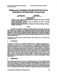
Figure 5: Performance Under Statistical Demand, Step TUFs
5.2 Performance with Statistical Demand
We now evaluate gMUA’s statistical timeliness assurances. The task settings used in our simulation study are summarized in Table 1. The table shows the task periods and the maximum utility (or Umax ) of the TUFs. For each task Ti ’s demand Yi , we generate normally distributed execution time demands. Task execution times are changed along with the total U D. We consider both step and heterogeneous TUF shapes as before. Task T1 T2 T3 T4 T5 T6
Pi 25 28 49 49 41 49
Table 1: Uimax 400 100 20 100 30 400
Task Settings ρi E(Yi ) 0.96 3.15 0.96 13.39 0.96 18.43 0.96 23.91 0.96 14.98 0.96 24.17
V ar(Yi ) 0.01 0.01 0.01 0.01 0.01 0.01
Figures 5(a) shows AUR and CMR of each task under increasing total U D of gMUA. For a task with step TUFs, task-level AUR and CMR are identical, as satisfying the critical time implies the accrual of a constant utility. But the system-level AUR and CMR are different as satisfying the critical time of each task does not always yield the same amount of utility. Figure 5(a) shows that all tasks under gMUA accrue 100% AUR and CMR within the global EDF’s bound (i.e., UD