On Partitioning Grids into Equal Parts

On Partitioning Grids into Equal Parts∗ S.L. Bezrukov Department of Math. and Comp. Sci. University of Paderborn D-33095 Paderborn, Germany B. Rovan† Department of Computer Science Comenius University 842 15 Bratislava, Slovakia

Abstract Let an edge cut partition the vertex set of an n-dimensional quadratic grid with the side length a into k subsets A1 , ..., Ak with ||Ai | − |Aj || ≤ 1. We consider the problem of determining the minimal size c(n, k, a) of such a cut and present its √ asymptotic c(n, k, a) ∼ nan−1 n k as a, k → ∞ and k/an → 0. The same asymptotic holds for partitioning of the n-dimensional torus. We present also some heuristics, which provide better partitioning for n = 2 and small k.

1

Introduction

Various aspects of graph partitioning are of a particular interest in theoretical computer science and they arise in various applications. In our paper we study partitioning of grids – a kind of graphs which appear quite naturally, e.g., in numerical computations. Application of the finite elements method for solving differential equations requires partitioning of the underlying area into simple figures - e.g. squares - and assigning the nodes of the partition to the processors of a parallel computing system. This leads to the problem of constructing an assignment in such a way that the total amount of computations would be equally distributed among the processors and the information flow between the processors would be minimized. In other words, one has to partition the vertex set of the ∗ This work was partially supported by the German Research Association (DFG) within the SFB 376 “Massive Parallelit¨ at: Algorithmen, Entwurfsmethoden, Anwendungen”. † Most of this research was done during this author’s stay at the University of Paderborn

1

underlying partition graph into a certain number of parts (corresponding to the number of processors in the system) consisting of equal number of vertices so, that the number of edges connecting the vertices of different parts is as small as possible. Graph partitioning problems are extensively studied in the literature. Many papers are devoted to partitioning of arbitrary graphs (e.g. [6, 7, 9]) and to the analysis of the complexity of partition problems. However, partitioning of some special graph classes often arising in practice is still not satisfactorily studied. Relatively many papers are devoted to partitioning of graphs into two parts and to computing the bisection width of such graphs, while the general case concerning the partitioning into more parts remains open. Grid-like graphs are naturally of particular importance for practice. Exact partitioning of grids into 2 parts was studied e.g. in [1, 3]. The paper [11] contains a number of other interesting results concerning partitioning of low-dimensional grids. Tori and their partitioning were studied in [4, 10], where the lower bounds are presented (see also [8]). The paper [2] deals with k-partitioning of the hypercube and contains some asymptotically optimal results for particular series of k. In our paper we study k-partitioning of n-dimensional a × · · · × a grids. Denoting the vertex set of such a grid via Gn , our problem is to construct for a given k a partition of the set Gn into k parts A1 , ..., Ak with ||Ai | − |Aj || ≤ 1. In other words 

an an ≤ |Ai | ≤ , k k 





i = 1, ..., k.

(1)

For such a partition A = {A1 , ..., Ak } denote ∇A = {(u, v) | u ∈ Ai , v ∈ Aj , i 6= j}, i.e. ∇A is the set of cutting edges in the partition A. We say that a partition A is optimal if |∇A| is the smallest possible and denote by ∇(n, k, a) the size of an optimal partition. We deal with the problem of finding the asymptotic of ∇(n, k, a) with n fixed and a, k → ∞. Our construction used in the proof of the upper bound provides a good partitioning when k is relatively large. For n = 2 we also present some heuristics, which for small k work better than the general construction. The paper is organized as follows. In the next section we introduce a continuous model for the partitioning problem and present an asymptotic for the continuous analog of the number of the cutting edges. These results are used in Section 3 to get the asymptotic of the minimal number of the cutting edges in the original discrete model. Section 4 is devoted to heuristics, which provide better results for the partitioning for small k. Some remarks in Section 5 conclude the paper.

2

2

The Continuous Model

We use the following continuous model for the partitioning problem. For n ≥ 2 replace the grid Gn by the a × · · · × a continuous n-dimensional cube Qn . By a rectilinear body in IRn we understand a measured area bounded by the hyperplanes of IRn parallel to the hyperplanes xi = 0, i = 1, ..., n, which we call basic hyperplanes. For a rectilinear body B ⊆ IRn denote by µB its volume and by ∂B the volume of its boundary. The volume of B and the volume of its boundary are the continuous analogs of the number of vertices of a subset of Gn and the size of the edge cut separating a set of vertices from its complement in Gn respectively. We start with the well-known isoperimetric inequality for the rectilinear bodies (cf. [3]). Lemma 1 Let n ≥ 2 and B ⊂ IRn be a rectilinear body. Then ∂B ≥ 2n (µB)

n−1 n

.

(2)

In particular, the boundary of the cube with volume µ(B) is minimal among the boundaries of rectilinear bodies having volume µ(B). Let Qn be partitioned by the basic hyperplanes into k rectilinear bodies B1 , ..., Bk having n volume ak each and denote Π = {B1 , ..., Bk }. Furthermore, denote by σΠ the volume of S B∈Π ∂B. Clearly σΠ is the continuous analog of the number of the cutting edges. Consider a problem of finding a partition Π of Qn into k rectilinear bodies having volume an each, so that σΠ is minimal. Denote this minimal value of σΠ by `(n, k, a). k Theorem 1 It holds: nan−1

√ n



k − 1 ≤ `(n, k, a) ≤ nan−1

√ n



k + cn ,

(3)

for some constant cn depending on n only. Proof. Consider first the lower bound. Let Π = {B1 , ..., Bk } be an optimal partition of Qn , and x be a point of the boundary1 of some Bi . Clearly, if x is also a boundary point of Qn , then it is a boundary point of no other body Bj in the partition, because each Bi is a rectilinear body. Otherwise, x is a common boundary point of exactly some two distinct bodies Bi and Bj . Therefore, k X

∂Bi = ∂Qn + 2 · σΠ = ∂Qn + 2 · `(n, k, a).

(4)

i=1 1

To simplify the argument we consider only the “internal” boundary points, meaning, e.g. in three dimensional case, that we disregard the edges and consider internal points of the faces only. This clearly does not affect the argument concerning the volume of the boundaries.

3

By Lemma 1, ∂Bi ≥ 2n (µBi )

n−1 n

= 2n an−1 k −

n−1 n

,

which after taking into consideration ∂Qn = 2nan−1 gives the lower bound in (3). Similar lower bound can be established using the approach of [5]. To get the upper bound in (3), consider first the case, when k = tn for some integer t ≥ 2. In this case one can partition each edge of Qn into t equal segments, which provides a partitioning of Qn into tn subcubes. This partition is optimal, because it reaches the lower bound in (3). Therefore, `(n, tn , a) = nan−1 (t − 1). In the case of arbitrary k we use induction on n. In the case n = 1 we extend the definition of the rectilinear body defining it as the union of nondisjoint line segments. Furthermore, for a partition Π of the line segment [0.a] into k rectilinear bodies define σΠ as the number of points separating the bodies. Then trivially holds: `(1, k, a) = k − 1 and so c1 = −1. Now assume that n ≥ 2 and k is large enough, i.e. k ≥ 2n . n

Represent k in the form k = tn +δ with 0 < δ < (t+1)n −tn and t ≥ 2. Denote a0 = tnt+δ a tn 0 0 n n and consider a a × · · · × a ×a rectangle Q ⊂ Q with volume n +δ a , containing the t | {z } n−1

origin of Qn , and let Q00 = Qn \ Q0 . Clearly, Q00 is a a × ·{z · · × a} ×(a − a0 ) rectangle. | n−1

We partition the rectangle Q0 into tn rectilinear bodies of size an /k by dividing each of its edges into t equal parts. To obtain the rest k − tn = δ parts of the partition we make a special partition of the rectangle Q00 using the fact that the length of one of its sides a − a0 = tnδ+δ a is relatively small and, as we shall see, even a simple partition of this rectangle does not affect the asymptotic of `(n, k, a). One has `(n, k, a) ≤ σΠ0 + σΠ00 + an−1 .

(5)

where Π0 , Π00 are the partitions of Q0 and Q00 respectively. Since each rectilinear body in the partition Π0 is a rectangle, one has σΠ0 = an−2 ((n − 1)a0 + a)(t − 1) ≤ nan−1 t.

(6)

To construct the partition Π00 of the rectangle Q00 we represent it as the cartesian product Q000 × (a − a0 ), where Q000 is the (n − 1)-dimensional cube with the side length a. Take an optimal partition of the cube Q000 into δ parts of equal size and for each part Bi000 of this partition construct a rectilinear body Bi00 = Bi000 × (a − a0 ), i = 1, ..., δ. The collection of the rectilinear bodies {Bi00 } forms the partition Π00 of Q00 . Therefore,   √ n−1 δ + cn−1 (7) σΠ00 = (a − a0 ) · `(n − 1, δ, a) ≤ (a − a0 )(n − 1)an−2 by induction. Since the function δ/(tn + δ) increases on δ and δ < (t + 1)n − tn ≤ bn tn−1  n for some bn with bn ≤ n n/2 , one has a − a0 =

δ (t + 1)n − tn bn a a ≤ a≤ . n n t +δ t t 4

(8)



Ci

G2 \ G0 .. .

G

0

.. .

Q0

Bi

Ai



Ci

a.

b.

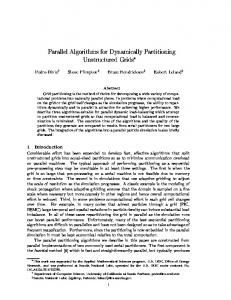
Figure 1: Partitioning of two-dimensional grid From (7) and (8) it follows σΠ00 ≤

q bn (n − 1) n−1 n−1 a t bn + cn−1 ≤ cn an−1 t 



√ for some cn depending on n only, which satisfies the recursion cn ≤ bn (n−1)( n−1 bn +cn−1 ) with c1 = −1. Substituting this and (6) into (5) gives the upper bound in (3). 2

3

Minimizing the Number of Cutting Edges

Consider first the 2-dimensional grids. In this particularly practical case we present first a construction providing a better constant c2 for the continuous model than above, and after that show how this construction can be modified for partitioning the discrete grids. Similar arguments work also in the higher-dimensional case. Let k ≥ 5 and let it be represented in the form k = t2 + δ with t ≥ 2 and 0 < δ < 2 (t + 1)2 − t2 = 2t + 1. Consider the subsquare Q0 ⊂ Q2 with side length t2t+δ a (cf. Fig. 3a) 2 2 and partition it as above in the optimal way into t2 parts B1 , ..., Bt2 of area t2a+δ = ak . To complete the partitioning of the whole square Q2 we have to partition the region Q2 \ Q0 into δ parts C1 , ..., Cδ of the same area. We make this partition as it is shown in Fig. 3a for the case of odd δ, where q the  cutting lines are depicted by the thin lines. Notice that t2 2 µCi >  , where  = 1 − t2 +δ a. This proves the correctness of the whole construction. The partition in the case of even δ is quite similar and therefore omitted.

5

Taking into account δ ≤ 2t, one has s

s

t2 t2 `(2, k, a) ≤ 2a 2 (t − 1) + (δ − 1) + 2a 2 t +δ t +δ   s √  δ  ≤ 2at + 1 − 1 − 2 aδ ≤ 2a k + 2 . t +δ Here in the last inequality we used t ≤

√

k and

√

1 − x ≥ 1 − x for 0 ≤ x ≤ 1.

Now let us return back to our original problem of partitioning of G2 . The lower √ bound (3) for the cardinality of the cut is still valid, and we rewrite it in the form 2a( k − 1) ≤ ∇(2, k, a). Concerning the upper bound, it is impossible to separate the grid just by direct lines as in our construction in Theorem 1 in general, because a2 may not be divisible by k. Thus, the rectangles in our construction will contain steps. In any case, it is easily seen that the number of steps is O(k), if each part of the partition is large enough. This leads to the following theorem: Theorem 2 It holds:

√ ∇(2, k, a) ∼ 2a k,

(9)

as a, k → ∞ and k/a2 → 0. Proof. We get the upper bound for ∇(2, k, a), using the above construction. However, the parts of the partition are not squares and rectangles in general and may contain steps of height 1. It is sufficient to show that the number of such steps is O(k). Indeed, in this case we would have an upper bound √ √ ∇(2, k, a) ≤ 2a( k + 1) + O(k) = 2a k(1 + o(1)), √ if k = o(a), which provides the asymptotic (9). We assume that k = t2 + δ with 0 ≤ δ < 2t and that k0 parts in our partition have cardinality m = ba2 /kc for some k0 > 0 and the rest k1 = k − k0 ≥ 0 parts are of cardinality da2 /ke = m + 1. We split the parts in the partition into 2 groups: the group A0 of t2 parts Ai and the group A00 of δ ≥ 0 parts Ci . Since t ≥ 2 then t2 ≥ 2t > δ and so without loss of generality we assume that all the parts Ci have the same cardinality. First we construct the parts of the group A0 . Let M = Ai ∈A0 |Ai | and let the number M be represented in the form M = b2 + r. Consider the set G0 ⊂ G2 of cardinality M shown in Fig. 3b and split it into t parts of cardinality bM/tc or bM/tc + 1 each. After that split each obtained part into subparts of cardinalities differing on 1. In the resulting partition of the set G0 into t2 parts, the cardinality of each part is either m or m + 1 or m + 2. If there are parts of cardinality m + 2, we take one vertex from such a set and assign it to arbitrary set of cardinality m. Clearly, the number of steps in the part A0 is O(t2 ) = O(k). P

6

Now split the vertex set G2 \ G0 into δ parts of the same size as it is shown in Fig. 3b. Clearly, the total number of steps in all parts Ci is O(δ) = O(k), which completes the proof. 2 Following similar arguments and using the construction of the upper bound in Theorem 1 one can ensure that the number of steps in partitioning of the n-dimensional grid Gn is O(nk), which in combination with (3) leads to the following result. Theorem 3 It holds:

√ n ∇(n, k, a) ∼ nan−1 k,

(10)

as n = const, a, k → ∞ and k/an → 0. We leave checking of the omitted details to the reader.

4

Heuristics

The basic idea is to make the decomposition by using a table of best known decompositions into smaller number of parts. It is expected to be used for decompositions into “small” √ number of parts, i.e., in decompositions into k parts, where k  k does not hold (i.e., the δ in the proof of Theorem 2 is not necessarily small) and the method from Section 2 does not give satisfactory results. We shall again consider decomposition of a rectangle in a continuous case. In the discrete case this amounts to the assumption that the length of each interval occurring in the construction is divisible into a required number of subintervals of equal length. Each subpart will be a rectangle with the sides parallel to the sides of the original rectangle. The heuristics can still be used in the discrete case, producing a decomposition into parts the sizes of which may differ by more than one. By replacing some straight line borders by “dogleg” borders one can try to obtain a correct decomposition without increasing the length of the borders too much.

4.1

Simple Heuristics

The following is a simplified version of the heuristics, illustrating the basic idea. Input: a and b, the sides of a rectangle parallel to the axes x and y respectively, and k, the number of parts into which the rectangle is to be decomposed. (We assume a ≤ b.) Assumed: A precomputed table is known, giving the best known decomposition of x by y rectangles into l parts of equal size, 2 ≤ l ≤ k − 1. In each case the total length of borders parallel to x and the total length of borders parallel to y is given. These give the cost of decomposition c(x, y; l). Due to the symmetry we can assume x ≤ y. 7

k = 2; (1,1)

k = 3; (2,1)

k = 4; (2,2)

k = 5; (3,2)

c(x, y; 2) = x

c(x, y; 3) = x + 23 y

c(x, y; 4) = x + y

c(x, y; 5) = 53 x + y

k = 6; (4,2)

k = 7; (5,2)

k = 8; (6,2)

k = 9; (6,3)

c(x, y; 8) = 2x + 74 y

c(x, y; 9) = 2x + 2y

c(x, y; 6) = 2x + y

c(x, y; 7) = 2x +

31 y 21

Figure 2: Partitions provided by Algorithm 1 Output: Decomposition of the a by b rectangle into k parts of equal size. Algorithm 1 1. For each i, 1 ≤ i ≤ k/2, do (a) Divide the rectangle a by b into two rectangles of the size a×( ki b) and a×( k−i b) k by a line parallel to a. (b) Use the table to get the best i-decomposition and the best (k − i)-decomposition of the new rectangles. Make the x direction parallel to a or b, whichever gives smaller border size. Call the resulting cost ci (a, b; k). 2. Choose i with the smallest ci (a, b; k) and output the corresponding decomposition. We illustrate this by giving a table for decomposing a square. For each k we give the decomposition (i, k − i) giving the minimal cost ci (a, b; k).

4.2

Improved Heuristics

The above approach is rather simplistic. It does not take into account, that for various values of the ratio x/y different decompositions into k parts may be needed to obtain 8

better results. Now we present a heuristic algorithm for constructing the “table of best decompositions”, that will take into account the values of x/y. In fact, we only present the algorithm for extending an existing table for decompositions into up to k − 1 equal parts into a table giving decompositions into k equal parts. Input: An integer k and the table Tk−1 giving the best known decomposition of x by y rectangles into l parts of equal size, 2 ≤ l ≤ k − 1, depending on the ratio of x and y. In each case the total length of borders parallel to x and the total length of borders parallel to y is given. These give the cost of the decomposition c(x, y; l). Due to the symmetry we can assume x ≤ y. Output: The table Tk . For the sake of presentation we refer to the rectangle to be decomposed into k parts (new entry in the table) as an a by b rectangle, assuming a ≤ b. The rectangles in the existing table are referred to as x by y rectangles. Algorithm 2 1. For each i, 1 ≤ i ≤ k/2, do (a) Divide the rectangle a by b into two rectangles of the size a×( ki b) and a×( k−i b) k by a line parallel to a. (b) Use the table to get all decompositions of each of the two rectangles obtained by placing each decomposition in both ways (x parallel to a and x parallel to b) for each interval for x/y in the table and each pairing of the i–decomposition and (k − i)–decomposition. (c) For each of the decompositions obtained compute the length of the border (the cost of decomposition) as a linear function in a and b and add to the list of potential decompositions. 2. Decompose the interval (0, 1] into subintervals for values of a/b using intersection points of the linear functions in the list of the potential decompositions. 3. Choose the best decomposition for each of the subintervals of (0, 1] and create the entry for k–decomposition in the table. We illustrate the above algorithm by the case where from a given T3 (see Fig. 4.2) a T4 is constructed. The ↑ and → indicate the orientation of the decomposition from T3 used. Thus 31 ↑ denotes the decomposition into three parts which is given for the first interval in T3 , i.e., (0, 32 ], placed as shown in T3 . Similarly 32 → denotes the decomposition into three parts which is given for the second interval in T3 , i.e., ( 23 , 1], placed turned 90 degrees, etc. We have the following decompositions of an a × b rectangle, following the Algorithm 2: 9

k = 2;

x y

∈ (0, 1]

c(x, y; 2) = x

k = 3;

x y

∈ (0, 23 ]

k = 3;

x y

∈ ( 23 , 1]

c(x, y; 3) = x + 23 y

c(x, y; 3) = 2x

Figure 3: Partitioning into 3 parts 1 + 31 ↑

1 + 31 →

1 + 32 ↑

1 + 32 →

c(a, b; 4) = 3a

c(a, b; 4) = a + 32 b

c(a, b; 4) = 2a + 12 b

c(a, b; 4) = 35 a + 34 b

Figure 4: Costs of partitioning into 4 parts Step 1, i = 1. Step 1, i = 2. We use the partition 2 → and 2 → which gives c(a, b; 4) = a + b (cf. the right partition in Fig. 4.2). The cases 2 ↑ and 2 →; 2 → and 2 ↑; and 2 ↑ and 2 ↑ clearly do not bring new decomposition type and we omit them here to save space. Step 2. The “crossing points” giving the decomposition of the interval (0, 1] for the values of ab 9 are 38 , 12 , 16 , and 34 . (For example, considering the first two decompositions in Fig. 4.2 we get from 3a = a + 23 b the “crossing point” 34 and the fact that the first decomposition is better than the second for ab ∈ (0, 34 ].) Step 3. The first decomposition is the best in (0, 12 ] and the last in [ 21 , 1]. Thus, the table T4 is obtained from T3 by appending the following entries: Analogously we obtain from T4 the entries in Fig. 4.2 which together with T4 form T5 . It is tedious to compute the above tables by hand and an implementation of the two 10

k = 4;

x y

∈ (0, 12 ]

k = 4;

c(x, y; 4) = 3x

x y

∈ ( 12 , 1]

c(x, y; 4) = x + y

Figure 5: Partitioning into 4 parts by Algorithm 2

k = 5;

x y

∈ (0, 25 ]

c(x, y; 5) = 4x

k = 5;

x y

∈ ( 25 , 35 ]

k = 5;

c(x, y; 5) = 2x + 45 y

x y

9 ∈ ( 35 , 10 ]

c(x, y; 5) = 53 x + y

k = 5;

9 ∈ ( 10 , 1]

c(x, y; 5) = x + 85 y

Figure 6: Partitioning into 5 parts by Algorithm 2

11

x y

Table 1: k-partitioning of the unit square k lower bound Algorithm 1 Algorithm 2

2 0.82 1 1

3 1.46 1.66 1.66

4 2 2 2

5 6 7 8 9 2.47 2.9 3.29 3.66 4 2.66 3 3.47 3.75 4 2.60

algorithms would be desirable. The following table compares the lengths of the boundary of a k partition of a unit square as estimated by the lower bound with those obtained by the two algorithms given above. Note that for the values of k, for which the partition was found using the above algorithms, the result is close to the lower bound. It is also to be noted that for k = 5 one can see that Algorithm 2 gives better partition.

5

Concluding Remarks

We studied k-partitioning of n-dimensional quadratic grids and found asymptotic for the minimal number of cutting edges. We restricted ourselves to considering the most practical case when the dimension of the grid is fixed. However, it would be also interesting to investigate the case when the dimension tends to infinity and a and k are fixed. In this case one has similar difficulties as in the partitioning of the hypercube [2] and some special constructions are required. We leave this problem for further consideration. The same method can be applied to partitioning of discrete tori (i.e. the Cartesian product of cycles). Our construction of the upper bound is applicable in this case as well. However, one has to add |∂Qn | = 2nan−1 to the bound. This clearly does not affect its asymptotic behavior since n = const, a, k → ∞ and k/an → 0. For the proof of the lower bound we can also use similar arguments as in the proof of Theorem 1. Instead of (4) we have k X

∂Bi = 2 · σΠ = 2 · `(n, k, a),

i=1

which leads asymptotically to the same lower bound under the assumptions above. Thus we have the following theorem: Corollary 1 The size of an optimal k-partition of the n-dimensional a × · · · × a tori is √ asymptotically equal to nan−1 n k, as n = const, a, k → ∞ and k/an → 0. Finally let us mention that the construction of the upper bound in Theorem 1 can be used for obtaining an upper bound for the Pin Limitation Problem (see [5] for further details).

12

References [1] Ahlswede R., Bezrukov S.L.: Edge isoperimetric theorems for integer point arrays. Appl. Math. Lett., 8 (1995), No. 2, 75–80. [2] Bezrukov S.L.: On k-partitioning the n-cube. Technical Report tr-rsfb-95-002, University of Paderborn, 1995. [3] Bollob´as B., Leader I.: An isoperimetric inequality on the discrete torus. SIAM J. Appl. Math., 3 (1990), 32–37. [4] Bollob´as B., Leader I.: Edge-isoperimetric inequalities in the grid. Combinatorica, 11 (1991), 299–314. [5] Cypher R.: Theoretical Aspects of VLSI Pin Limitations. SIAM J. Comput., 22 (1993) 356–378. [6] Diekmann R., L¨ uling R., Monien B., Spr¨aner C.: Combining Helpful Sets and Parallel Simulated Annealing for the Graph-Partitioning Problem. Int. J. Parallel Algorithms and Applications, (to appear). [7] Diekmann R., Meyer D., Monien B.: Parallel Decomposition of Unstructured FEMMeshes. In: Proc. of IRREGULAR’95, Springer LNCS 980 (1995), 199–215. [8] Gilbert J.R., Miller G.L., Teng S.-H.: Geometric Mesh Partitioning: Implementation and Experiments. In: Proc. of IPPS’95, 1995. [9] Liou K.P., Pothen A., Simon H.D.: Partitioning sparse matrices with eigenvectors of graphs. SIAM J. on Matrix Anal. and Appl., 11 (1990), 430–452. [10] Mao W., Nicol D.M.: On k-ary n-cubes: Theory and Applications. In: Proc. of IPPS’95. [11] Rolim J., S´ ykora O., Vrt’o I.: Optimal Cutwidth and Bisection Width of 2- and 3-Dimensional Meshes. In: Proc. of WG’95.

13