Dec 30, 2008 - An [[n, k, r, d]]q subsystem code is a decomposition of the subspace Q into a tensor product of two vector spaces A ...... New York: John Wiley,. 2005. ..... [181] A. M. Stephens, Z. W. E. Evans, S. J. Devitt, and L. C. L. Hollenberg.
arXiv:0812.5104v1 [cs.IT] 30 Dec 2008
On Quantum and Classical Error Control Codes: Constructions and Applications
Salah A. Aly
Major Subject: Computer Science c All Rights Reserved
2008
On Quantum and Classical Error Control Codes: Constructions and Applications Parts of this work were submitted to the Department of Computer Science at Texas A&M University for the degree of doctoral of Philosophy on Fall 2007. Some other parts were added later without peer reviews. The document is reformatted. Please report all typos or errors to the author with all due haste.
To my family and teachers
Abstract
It is conjectured that quantum computers are able to solve certain problems more quickly than any deterministic or probabilistic computer. For instance, Shor’s algorithm is able to factor large integers in polynomial time on a quantum computer. A quantum computer exploits the rules of quantum mechanics to speed up computations. However, it is a formidable task to build a quantum computer, since the quantum mechanical systems storing the information unavoidably interact with their environment. Therefore, one has to mitigate the resulting noise and decoherence effects to avoid computational errors. In this work, I study various aspects of quantum error control codes – the key component of fault-tolerant quantum information processing. I present the fundamental theory and necessary background of quantum codes and construct many families of quantum block and convolutional codes over finite fields, in addition to families of subsystem codes. This work is organized into these parts: Quantum Block Codes. After introducing the theory of quantum block codes, I establish conditions when BCH codes are self-orthogonal (or dual-containing) with respect to Euclidean and Hermitian inner products. In particular, I derive two families of nonbinary quantum BCH codes using the stabilizer formalism. I study duadic codes and establish the existence of families of degenerate quantum codes, as well as families of quantum codes derived from projective geometries. Subsystem Codes. Subsystem codes form a new class of quantum codes in which the underlying classical codes do not need to be self-orthogonal. I give an introduction to subsystem codes and present several methods for subsystem code constructions. I derive families of subsystem codes from classical BCH and RS codes and establish a family of optimal MDS subsystem codes. I establish propagation rules of subsystem codes and construct tables of upper and lower bounds on subsystem code parameters. Quantum Convolutional Codes. Quantum convolutional codes are particularly well-suited for communication applications. I develop the theory of quantum convolutional codes and give families of quantum convolutional codes based on RS codes. Furthermore, I establish a bound on the code parameters of quantum convolutional codes – the generalized Singleton bound. I develop a general framework for deriving convolutional codes from block codes and use it to derive families of non-catastrophic quantum convolutional codes from BCH codes. Quantum and Classical LDPC Codes. LDPC codes are a class of modern error control codes that can be decoded using iterative decoding algorithms. In this part, I derive classes of quantum LDPC codes based on finite geometries, Latin squares and combinatorial objects. In addition, I construct families of LDPC codes derived from classical BCH codes and elements of cyclotomic cosets. Asymmetric Quantum Codes. Recently, the theory of quantum error control codes has been extended to include quantum codes over asymmetric quantum channels — qubit-flip and phase-shift errors may occur with different probabilities. I derive families of asymmetric quantum codes derived from classical BCH and RS codes over finite fields. In addition, I derive a generic method to derive asymmetric quantum cyclic codes.
iii
Contents
1 Introduction 1.1 Background . . . . 1.2 Quantum Codes . 1.3 Problem Statement 1.4 Work Outline . . .
. . . .
. . . .
. . . .
. . . .
. . . .
. . . .
. . . .
. . . .
. . . .
. . . .
. . . .
. . . .
. . . .
. . . .
. . . .
. . . .
. . . .
. . . .
. . . .
. . . .
. . . .
. . . .
. . . .
. . . .
. . . .
. . . .
. . . .
. . . .
. . . .
. . . .
. . . .
1 1 2 3 5
2 Background 2.1 Classical Coding Theory . . . . . . . . . 2.1.1 Bounds on the Code Parameters 2.1.2 Families of Codes . . . . . . . . . 2.2 Quantum Error Control Codes . . . . . 2.2.1 Quantum Block Codes . . . . . . 2.2.2 Subsystem Codes . . . . . . . . . 2.2.3 Quantum Convolutional Codes . 2.3 Fault Tolerant Quantum Computing . .
. . . . . . . .
. . . . . . . .
. . . . . . . .
. . . . . . . .
. . . . . . . .
. . . . . . . .
. . . . . . . .
. . . . . . . .
. . . . . . . .
. . . . . . . .
. . . . . . . .
. . . . . . . .
. . . . . . . .
. . . . . . . .
. . . . . . . .
. . . . . . . .
. . . . . . . .
. . . . . . . .
. . . . . . . .
. . . . . . . .
. . . . . . . .
. . . . . . . .
. . . . . . . .
. . . . . . . .
. . . . . . . .
. . . . . . . .
. . . . . . . .
. . . . . . . .
. . . . . . . .
. . . . . . . .
6 6 7 8 8 8 9 10 10
I
. . . .
. . . .
. . . .
. . . .
. . . .
. . . .
. . . .
. . . .
. . . .
. . . .
. . . .
Quantum Block Codes
11
3 Fundamentals of Quantum Block Codes 3.1 Stabilizer Codes . . . . . . . . . . . . . . . . . . . . . . . . . . 3.1.1 Error Bases . . . . . . . . . . . . . . . . . . . . . . . . . 3.1.2 Stabilizer Codes . . . . . . . . . . . . . . . . . . . . . . 3.1.3 Stabilizer and Error Correction . . . . . . . . . . . . . . 3.1.4 Encoding Quantum Codes . . . . . . . . . . . . . . . . . 3.2 Deriving Quantum Codes from Self-orthogonal Classical Codes 3.2.1 Codes over Fq . . . . . . . . . . . . . . . . . . . . . . . . 3.2.2 Codes over Fq2 . . . . . . . . . . . . . . . . . . . . . . . . 3.3 Bounds on Quantum Codes . . . . . . . . . . . . . . . . . . . . 3.4 Perfect Quantum Codes . . . . . . . . . . . . . . . . . . . . . .
. . . . . . . . . .
. . . . . . . . . .
. . . . . . . . . .
. . . . . . . . . .
. . . . . . . . . .
. . . . . . . . . .
. . . . . . . . . .
. . . . . . . . . .
. . . . . . . . . .
. . . . . . . . . .
. . . . . . . . . .
. . . . . . . . . .
. . . . . . . . . .
. . . . . . . . . .
. . . . . . . . . .
. . . . . . . . . .
. . . . . . . . . .
12 12 13 13 14 15 15 16 17 17 19
4 Quantum BCH Codes 4.1 BCH Codes . . . . . . . . . . . . . . . . . . . . . . . 4.2 Dimension and Minimum Distance . . . . . . . . . . 4.2.1 Dimension . . . . . . . . . . . . . . . . . . . . 4.2.2 Distance Bounds . . . . . . . . . . . . . . . . 4.3 Euclidean Dual Codes . . . . . . . . . . . . . . . . . 4.4 Hermitian Dual Codes . . . . . . . . . . . . . . . . . 4.5 Families of Quantum BCH Codes . . . . . . . . . . . 4.6 Quantum BCH from Self-orthogonal Product Codes 4.7 Conclusions and Discussion . . . . . . . . . . . . . .
. . . . . . . . .
. . . . . . . . .
. . . . . . . . .
. . . . . . . . .
. . . . . . . . .
. . . . . . . . .
. . . . . . . . .
. . . . . . . . .
. . . . . . . . .
. . . . . . . . .
. . . . . . . . .
. . . . . . . . .
. . . . . . . . .
. . . . . . . . .
. . . . . . . . .
. . . . . . . . .
. . . . . . . . .
21 21 23 23 24 25 26 27 28 29
1
. . . . . . . . .
. . . . . . . . .
. . . . . . . . .
. . . . . . . . .
. . . . . . . . .
. . . . . . . . .
2
Contents
5 Quantum Duadic Codes 5.1 Introduction . . . . . . . . . . . . . . . . . 5.2 Classical Duadic Codes . . . . . . . . . . . 5.3 Quantum Duadic Codes – Euclidean Case 5.3.1 Basic Code Constructions . . . . . 5.3.2 Degenerate Codes . . . . . . . . . 5.4 Quantum Duadic Codes – Hermitian Case 5.4.1 Basic Code Constructions . . . . . 5.4.2 Degenerate Codes . . . . . . . . . 5.5 Conclusion . . . . . . . . . . . . . . . . .
. . . . . . . . .
. . . . . . . . .
. . . . . . . . .
. . . . . . . . .
. . . . . . . . .
. . . . . . . . .
. . . . . . . . .
. . . . . . . . .
. . . . . . . . .
. . . . . . . . .
. . . . . . . . .
. . . . . . . . .
. . . . . . . . .
. . . . . . . . .
. . . . . . . . .
. . . . . . . . .
. . . . . . . . .
. . . . . . . . .
. . . . . . . . .
. . . . . . . . .
. . . . . . . . .
. . . . . . . . .
. . . . . . . . .
. . . . . . . . .
. . . . . . . . .
. . . . . . . . .
. . . . . . . . .
. . . . . . . . .
. . . . . . . . .
30 30 31 32 32 33 34 34 35 35
6 Quantum Projective Geometry Codes 6.1 Projective Reed-Muller Codes . . . . . . 6.2 Quantum Projective Reed-Muller Codes 6.3 Puncturing Quantum Codes . . . . . . . 6.4 Conclusion and Discussion . . . . . . . .
. . . .
. . . .
. . . .
. . . .
. . . .
. . . .
. . . .
. . . .
. . . .
. . . .
. . . .
. . . .
. . . .
. . . .
. . . .
. . . .
. . . .
. . . .
. . . .
. . . .
. . . .
. . . .
. . . .
. . . .
. . . .
. . . .
. . . .
. . . .
. . . .
36 36 37 38 39
II
. . . .
Subsystem Codes
40
7 Subsystem Codes 7.1 Introduction . . . . . . . . . . . . . . . . . . . 7.2 Subsystem Codes . . . . . . . . . . . . . . . . 7.3 Bounds on Pure Subsystem Code Parameters 7.3.1 Quantum Singleton Bound . . . . . . 7.3.2 Quantum Hamming Bound . . . . . .
. . . . .
. . . . .
. . . . .
. . . . .
. . . . .
. . . . .
. . . . .
. . . . .
. . . . .
. . . . .
. . . . .
. . . . .
. . . . .
. . . . .
. . . . .
. . . . .
. . . . .
. . . . .
. . . . .
. . . . .
. . . . .
. . . . .
. . . . .
. . . . .
. . . . .
. . . . .
. . . . .
41 41 42 43 43 44
8 Subsystem Code Constructions 8.1 Introduction . . . . . . . . . . . . . . . . 8.2 Subsystem Code Constructions . . . . . 8.3 Trading Dimensions of Subsystem Codes 8.4 MDS Subsystem Codes . . . . . . . . . . 8.5 Conclusion and Discussion . . . . . . . .
. . . . .
. . . . .
. . . . .
. . . . .
. . . . .
. . . . .
. . . . .
. . . . .
. . . . .
. . . . .
. . . . .
. . . . .
. . . . .
. . . . .
. . . . .
. . . . .
. . . . .
. . . . .
. . . . .
. . . . .
. . . . .
. . . . .
. . . . .
. . . . .
. . . . .
. . . . .
. . . . .
. . . . .
46 46 46 47 50 52
. . . . . . . . . . . . . . . . . . . . . . . . . . . . [[6, 1, 1, 3]]3 . . . . . . .
. . . . . .
. . . . . .
. . . . . .
. . . . . .
. . . . . .
. . . . . .
. . . . . .
. . . . . .
. . . . . .
. . . . . .
. . . . . .
. . . . . .
. . . . . .
. . . . . .
. . . . . .
. . . . . .
. . . . . .
. . . . . .
. . . . . .
. . . . . .
. . . . . .
. . . . . .
. . . . . .
. . . . . .
. . . . . .
. . . . . .
. . . . . .
54 54 55 57 59 62 65
10 Propagation Rules and Tables of Subsystem Code Constructions 10.1 Introduction . . . . . . . . . . . . . . . . . . . . . . . . . . . . . . . . 10.2 Upper and Lower Bounds on Subsystem Code Parameters . . . . . . 10.3 Pure Subsystem Code Constructions . . . . . . . . . . . . . . . . . . 10.4 Propagation Rules of Subsystem Codes . . . . . . . . . . . . . . . . . 10.5 Conclusion and Discussion . . . . . . . . . . . . . . . . . . . . . . . .
. . . . .
. . . . .
. . . . .
. . . . .
. . . . .
. . . . .
. . . . .
. . . . .
. . . . .
. . . . .
. . . . .
. . . . .
. . . . .
. . . . .
66 66 66 68 69 78
9 Families of Subsystem Codes 9.1 Introduction . . . . . . . . . . . . 9.2 Cyclic Subsystem Codes . . . . . 9.3 Subsystem BCH Codes . . . . . . 9.4 Subsystem RS Codes . . . . . . . 9.5 Subsystem Codes [[8, 1, 2, 3]]2 and 9.6 Conclusion and Discussion . . . .
III
. . . . .
. . . . .
Quantum Convolutional Codes
11 Quantum Convolutional Codes 11.1 Introduction . . . . . . . . . . . . . . . . . . . . . . . . . . . . . . . . . . . . . . . . . . . . . . 11.2 Previous Work on QCC . . . . . . . . . . . . . . . . . . . . . . . . . . . . . . . . . . . . . . . 11.3 Background on Convolutional Codes . . . . . . . . . . . . . . . . . . . . . . . . . . . . . . . .
79 80 80 80 81
Contents
. . . . . . .
. . . . . . .
. . . . . . .
. . . . . . .
. . . . . . .
. . . . . . .
. . . . . . .
. . . . . . .
. . . . . . .
. . . . . . .
. . . . . . .
. . . . . . .
. . . . . . .
81 82 83 85 87 87 88
12 Quantum Convolutional Codes Derived from Reed-Solomon Codes 12.1 Convolutional GRS Stabilizer Codes . . . . . . . . . . . . . . . . . . . . 12.2 Quantum Convolutional Codes from RS Codes . . . . . . . . . . . . . . 12.3 Convolutional Codes from Quasi-Cyclic Subcodes of Reed-Muller Codes 12.4 Quantum Convolutional Codes from QC RM Codes . . . . . . . . . . . 12.5 Conclusion and Discussion . . . . . . . . . . . . . . . . . . . . . . . . . .
. . . . .
. . . . .
. . . . .
. . . . .
. . . . .
. . . . .
. . . . .
. . . . .
. . . . .
. . . . .
. . . . .
. . . . .
89 89 91 92 94 94
13 Quantum Convolutional Codes derived from BCH Codes 13.1 Introduction . . . . . . . . . . . . . . . . . . . . . . . . . . . . . . . . . . . . . 13.2 Construction of Convolutional Codes from Block Codes . . . . . . . . . . . . 13.3 Convolutional BCH Codes . . . . . . . . . . . . . . . . . . . . . . . . . . . . . 13.3.1 Unit Memory Convolutional BCH Codes . . . . . . . . . . . . . . . . . 13.3.2 Hole’s Convolutional BCH Codes . . . . . . . . . . . . . . . . . . . . . 13.4 Constructing Quantum Convolutional Codes from Convolutional BCH Codes 13.5 QCC from Product Codes . . . . . . . . . . . . . . . . . . . . . . . . . . . . . 13.6 Efficient Encoding and Decoding Circuits of QCC-BCH . . . . . . . . . . . . 13.7 Conclusion and Discussion . . . . . . . . . . . . . . . . . . . . . . . . . . . . .
. . . . . . . . .
. . . . . . . . .
. . . . . . . . .
. . . . . . . . .
. . . . . . . . .
. . . . . . . . .
. . . . . . . . .
. . . . . . . . .
95 . 95 . 96 . 97 . 97 . 99 . 99 . 101 . 101 . 102
11.4 11.5 11.6 11.7
IV
11.3.1 Overview . . . . . . . . . . . . . . . 11.3.2 Algebraic Structure of Convolutional 11.3.3 Duals of Convolutional Codes . . . . Quantum Convolutional Codes . . . . . . . CSS Code Constructions . . . . . . . . . . . QCC Singleton Bound . . . . . . . . . . . . QCC Example . . . . . . . . . . . . . . . .
3
. . . . Codes . . . . . . . . . . . . . . . . . . . .
. . . . . . .
. . . . . . .
. . . . . . .
. . . . . . .
. . . . . . .
. . . . . . .
. . . . . . .
. . . . . . .
. . . . . . .
. . . . . . .
. . . . . . .
Quantum and Classical LDPC Codes
103
14 A Class of Quantum LDPC Codes Constructed From Finite Geometries 14.1 Introduction . . . . . . . . . . . . . . . . . . . . . . . . . . . . . . . . . . . . . 14.2 LDPC Code Constructions and Finite Geometries . . . . . . . . . . . . . . . 14.2.1 LDPC Codes . . . . . . . . . . . . . . . . . . . . . . . . . . . . . . . . 14.2.2 Finite Geometry . . . . . . . . . . . . . . . . . . . . . . . . . . . . . . 14.2.3 Adapting the Matrix HEG−II to be Self-orthogonal . . . . . . . . . . 14.2.4 Characteristic Vectors and Matrices . . . . . . . . . . . . . . . . . . . 14.3 Constructing Self-Orthogonal Cyclic LDPC Codes from Euclidean Geometry 14.3.1 Euclidean Geometry EG(m, q) . . . . . . . . . . . . . . . . . . . . . . 14.3.2 QC LDPC Codes . . . . . . . . . . . . . . . . . . . . . . . . . . . . . . 14.3.3 Self-orthogonal QC LDPC Codes . . . . . . . . . . . . . . . . . . . . . 14.4 Quantum LDPC Block Codes . . . . . . . . . . . . . . . . . . . . . . . . . . . 14.5 Conclusion . . . . . . . . . . . . . . . . . . . . . . . . . . . . . . . . . . . . .
. . . . . . . . . . . .
. . . . . . . . . . . .
. . . . . . . . . . . .
. . . . . . . . . . . .
. . . . . . . . . . . .
. . . . . . . . . . . .
. . . . . . . . . . . .
. . . . . . . . . . . .
. . . . . . . . . . . .
104 104 105 105 105 106 107 107 107 109 109 110 111
15 Quantum LDPC Codes Derived from Latin Squares 15.1 Introduction . . . . . . . . . . . . . . . . . . . . . . . . 15.2 Classical and Quantum LDPC Codes . . . . . . . . . . 15.2.1 Quantum LDPC Codes . . . . . . . . . . . . . 15.2.2 Classical LDPC Codes . . . . . . . . . . . . . . 15.3 Constructing LDPC Codes From Latin Squares . . . . 15.3.1 Latin Square . . . . . . . . . . . . . . . . . . . 15.3.2 A Class of LDPC . . . . . . . . . . . . . . . . . 15.3.3 Parameters of LDPC Codes . . . . . . . . . . . 15.4 Quantum LDPC Block Codes . . . . . . . . . . . . . . 15.5 Discussion . . . . . . . . . . . . . . . . . . . . . . . . . 15.6 Conclusion . . . . . . . . . . . . . . . . . . . . . . . .
. . . . . . . . . . .
. . . . . . . . . . .
. . . . . . . . . . .
. . . . . . . . . . .
. . . . . . . . . . .
. . . . . . . . . . .
. . . . . . . . . . .
. . . . . . . . . . .
. . . . . . . . . . .
112 112 113 113 113 115 115 116 117 119 120 120
. . . . . . . . . . .
. . . . . . . . . . .
. . . . . . . . . . .
. . . . . . . . . . .
. . . . . . . . . . .
. . . . . . . . . . .
. . . . . . . . . . .
. . . . . . . . . . .
. . . . . . . . . . .
. . . . . . . . . . .
. . . . . . . . . . .
. . . . . . . . . . .
. . . . . . . . . . .
4
Contents
16 Families of LDPC Codes Derived from Nonprimitive BCH Codes and Cyclotomic Cosets121 16.1 Introduction . . . . . . . . . . . . . . . . . . . . . . . . . . . . . . . . . . . . . . . . . . . . . . 121 16.2 Constructing LDPC Codes . . . . . . . . . . . . . . . . . . . . . . . . . . . . . . . . . . . . . 122 16.2.1 Definitions . . . . . . . . . . . . . . . . . . . . . . . . . . . . . . . . . . . . . . . . . . 122 16.2.2 Regular LDPC Codes . . . . . . . . . . . . . . . . . . . . . . . . . . . . . . . . . . . . 123 16.3 LDPC Codes based on BCH Codes . . . . . . . . . . . . . . . . . . . . . . . . . . . . . . . . . 124 16.3.1 Type-I Construction . . . . . . . . . . . . . . . . . . . . . . . . . . . . . . . . . . . . . 125 16.4 LDPC Codes Based on Cyclotomic Cosets . . . . . . . . . . . . . . . . . . . . . . . . . . . . . 127 16.4.1 Type-II Construction . . . . . . . . . . . . . . . . . . . . . . . . . . . . . . . . . . . . 128 16.5 Simulation Results . . . . . . . . . . . . . . . . . . . . . . . . . . . . . . . . . . . . . . . . . . 129 16.6 Conclusion . . . . . . . . . . . . . . . . . . . . . . . . . . . . . . . . . . . . . . . . . . . . . . 129
V
Applications
17 Asymmetric Quantum BCH Codes 17.1 Introduction . . . . . . . . . . . . . . . . . . . 17.2 Asymmetric Quantum Codes . . . . . . . . . 17.2.1 Higher Fields and Total Error Groups 17.3 Asymmetric Quantum BCH and RS Codes . 17.3.1 AQEC-BCH . . . . . . . . . . . . . . . 17.3.2 RS Codes . . . . . . . . . . . . . . . . 17.4 Illustrative Example . . . . . . . . . . . . . . 17.5 Conclusion and Discussion . . . . . . . . . . .
130 . . . . . . . .
. . . . . . . .
. . . . . . . .
. . . . . . . .
. . . . . . . .
. . . . . . . .
. . . . . . . .
. . . . . . . .
. . . . . . . .
. . . . . . . .
. . . . . . . .
. . . . . . . .
. . . . . . . .
. . . . . . . .
. . . . . . . .
. . . . . . . .
. . . . . . . .
. . . . . . . .
131 131 132 133 135 136 137 138 139
18 Asymmetric Quantum Cyclic Codes 18.1 Introduction . . . . . . . . . . . . . . . . . . . . . . . . . . . . . 18.2 Classical Cyclic Codes . . . . . . . . . . . . . . . . . . . . . . . 18.3 Asymmetric Quantum Cyclic Codes . . . . . . . . . . . . . . . 18.3.1 AQEC Based on Generator Polynomials of Cyclic Codes 18.3.2 Cyclic AQEC Using the Defining Sets Extension . . . . 18.4 AQEC Based on Two Cyclic Codes . . . . . . . . . . . . . . . . 18.5 Conclusion and Discussion . . . . . . . . . . . . . . . . . . . . .
. . . . . . .
. . . . . . .
. . . . . . .
. . . . . . .
. . . . . . .
. . . . . . .
. . . . . . .
. . . . . . .
. . . . . . .
. . . . . . .
. . . . . . .
. . . . . . .
. . . . . . .
. . . . . . .
. . . . . . .
. . . . . . .
. . . . . . .
140 140 140 141 141 142 144 144
. . . . . . . .
. . . . . . . .
. . . . . . . .
. . . . . . . .
. . . . . . . .
. . . . . . . .
. . . . . . . .
. . . . . . . .
. . . . . . . .
List of Figures
3.1
The relationship between a quantum stabilizer code Q and a classical code C, where C ⊆ C ⊥ .
15
7.1
A quantum code Q is decomposed into two subsystem A (info) and B (gauge) . . . . . . . . .
42
8.1 8.2
Subsystem code parameters from classical codes . . . . . . . . . . . . . . . . . . . . . . . . . . Stabilizer and subsystem codes based on classical codes . . . . . . . . . . . . . . . . . . . . .
48 51
14.1 Euclidean geometry with points n = 4 and lines l = 6 . . . . . . . . . . . . . . . . . . . . . . . 105 14.2 (a) EG with n = 4 points and l = 6 lines (b) The Tanner graph of a self-orthogonal H matrix. 106 15.1 Constructing LDPC codes based on elements of a finite field (Latin Square) . . . . . . . . . . 118 15.2 Performance of a (4,30) LDPC code with parameters (156,180) based on Latin squares . . . . 118 16.1 Type I: Performance of an (4,31) LDPC code with rate 27/31 and code size (837, 961). . . . 129 17.1 Constructions of asymmetric quantum codes based on two classical codes C1 and C2 . . . . . 135 18.1 Constructions of asymmetric quantum codes based on two classical cyclic codes . . . . . . . . 142
5
List of Tables
9.1 9.2 9.3 9.4 9.5
Subsystem BCH codes that are derived using the Euclidean construction . . . . . . . Subsystem BCH codes that are derived with the help of the Hermitian construction Optimal pure subsystem codes . . . . . . . . . . . . . . . . . . . . . . . . . . . . . . Reed-Solomon(RS) subsystem codes . . . . . . . . . . . . . . . . . . . . . . . . . . . Families of subsystem codes from stabilizer codes . . . . . . . . . . . . . . . . . . . .
. . . . .
. . . . .
. . . . .
. . . . .
. . . . .
59 60 62 63 65
10.1 Existence of subsystem propagation rules . . . . . . . . . . . . . . . . . . . . . . . . . . . . . 10.2 Upper bounds on subsystem code parameters using linear programming, q = 2 . . . . . . . . 10.3 Upper bounds on subsystem code parameters using linear programming, q = 3 . . . . . . . .
75 76 78
16.1 Parameters of LDPC codes derived from NP BCH codes . . . . . . . . . . . . . . . . . . . . . 127 17.1 Families of asymmetric quantum BCH codes [31] . . . . . . . . . . . . . . . . . . . . . . . . . 137 18.1 Families of asymmetric quantum Cyclic codes . . . . . . . . . . . . . . . . . . . . . . . . . . . 143
6
Acknowledgement
This work would not be a reality without the kind people whom I met during my graduate studies. I thank my advisor Dr. Andreas Klappenecker for his support, guidance, and patience. He kindly introduced me to this pioneering research. Andreas taught me how to write high quality research papers. Throughout countless emails, I cannot remember how many times I thought my code constructions and paper drafts were good enough, and he kindly challenged me to make them correct and outstanding. I thank all my committee members: Dr. M. Suhail Zubairy, Dr. Mahmoud El-Halwagi, Dr. Rabi Mahapatra, and Dr. Andrew Jiang. They were all supportive and kind. A special gratefulness goes to my mentor Dr. El-Halwagi for his encouragement. He was always an inspiration for me, whenever I faced tough times. I thank Zhenning Kong, Pradeep K. Sarvepalli, and Ahmad El-Guindy. I thank Martin Roetteler and Marcus Grassl for their collaboration. I would like to thank Emina Soljanin and the Mathematical Science Research Group at Bell Labs & Alcatel-Lucent. In a weighty remarkable document like this where the precision of every word counts with caution; remaining silent is too difficult. During the last five years of my life, I was undoubtedly isolated from people and life. Words can not describe how I felt. I would like to thank my parents and extended family members for their patience while I was away from them for many unseen years. Absolutely, this work is dedicated to them and I also wish this work will ignite a light for my nephews and all youth in my home city to encourage them to learn. Finally, from infancy until now, I have always been blessed by the prayers of my relatives and elders; I can now be sure that my work is not based on my cleverness or intelligence. I owe all praise, gratitude, and everything to Him. Salah A. Aly December 1, 2007.
7
CHAPTER
1
Introduction
Quantum computing is a relatively new interdisciplinary field that has recently attracted many researchers from physics, mathematics, and computer science. The main idea of quantum computing is to utilize the laws of quantum physics to perform fast computations. Quantum information processing can be beneficial in numerous applications, such as secure key exchange or quick search. Arguably, one of the most attractive features is that quantum algorithms are conjectured to solve certain computational problems exponentially faster than any classical algorithm. For instance, Shor’s quantum algorithm can factor integers faster than any known classical algorithm. Quantum information is represented by the states of quantum mechanical systems. Since the informationcarrying quantum systems will inevitably interact with their environment, one has to deal with decoherence effects that tend to destroy the stored information. Hence, it is infeasible to perform quantum computations without introducing techniques to remedy this dilemma. One method is to apply fault-tolerant operations that make the computations permissible under a certain threshold value. These fault-tolerant techniques employ quantum error control codes to protect quantum information. The main contribution of this work is the development of novel techniques for quantum error control, including the construction of numerous quantum error control codes to guard quantum information.
1.1
Background
The state space of a discrete quantum mechanical system is given by a finite-dimensional Hilbert space, namely by a finite-dimensional complex vector space that is equipped with the standard Hermitian inner product. The states of the quantum system are assumed to be vectors of unit length in the induced norm. Any quantum mechanical operation other than a measurement is given by a unitary linear operation. For quantum information processing, one chooses a fixed orthonormal basis of the state space of the quantum mechanical system, called the computational basis. The basis vectors represent classical information that is processed by the quantum computer. To fix ideas, consider a quantum system with two-dimensional state space C2 . The basis vectors � � � � 1 0 v0 = , v1 = 0 1 can be used to represent the classical bits 0 and 1. As the indices of the basis vectors can be difficult to read, it is customary in quantum information processing to use Dirac’s ket notation for the basis vectors; namely, the vector v0 is denoted by |0i and the vector v1 is denoted by |1i. Therefore, any possible state of such a two-dimensional quantum system is given by a linear combination of the form � � a a |0i + b |1i = , where a, b ∈ C and |a|2 + |b|2 = 1, b 1
2
Chapter 1: Introduction
as any vector of unit length is a possible state. One refers to the state vector of a two-dimensional quantum system as a quantum bit or qubit. The superposition or linear combination of the basis vectors |0i and |1i of a quantum bit is one marked difference between classical and quantum information processing. One can measure a quantum bit in the computational basis. Such a measurement of a quantum bit in the state a |0i + b |1i leaves the quantum bit with a probability of |a|2 in state |0i and with probability |b|2 in state |1i. Furthermore, the outcome of this probabilistic operation is recorded as a measurement result. In quantum information processing, the operations manipulating quantum bits follow the rules of quantum mechanics, that is, an operation that is not a measurement must be realized by a unitary operator. For example, a quantum bit can be flipped by a quantum NOT gate X that transfers the qubits |0i and |1i to |1i and |0i, respectively. Thus, this operation acts on a general quantum state as follows. X(a |0i + b |1i) = a |1i + b |0i .
�
� 0 1 . 1 0 Other popular operations include the phase flip Z, the combined bit and phase-flip Y , and the Hadamard gate H, which are represented with respect to the computational basis by the matrices � � � � � � 1 1 1 1 0 0 −i . Z= ,Y = ,H = √ 1 −1 0 −1 i 0 2 With respect to the computational basis, the quantum NOT gate X is represented by the matrix
The state space of a joint quantum system is described by the tensor product of the state spaces of its parts. Consequently, a quantum register of length n, which is by definition a combination of n qubits, can be represented by the normalized complex linear combination of the 2n mutually orthogonal basis states in n C2 , namely as a linear combination of the vectors |ψi = |ψ1 i ⊗ |ψ2 i ⊗ ... ⊗ |ψn i = |ψ1 ψ2 ...ψn i where |ψi i ∈ {|0i , |1i}. Operations acting on two (or more) quantum bits include the controlled not operation CNOT, which realizes the map |00i 7→ |00i , |01i 7→ |01i , |10i 7→ |11i , |11i 7→ |10i . In the computational basis, the CNOT operation is described 1 0 0 0 1 0 CN OT = 0 0 0 0 0 1
1.2
by the matrix 0 0 . 1 0
Quantum Codes
Quantum error control codes like their classical counterparts are means to protect quantum information against noise and decoherence. Quantum codes can be classified into additive or nonadditive codes. If the code is defined based on an abelian subgroup (stabilizer), then it is called an additive (stabilizer) code. The structure and construction of additive codes are well-known. Additive codes are also defined over a vector space, therefore addition (or subtraction) of two codewords is also a valid codeword in the codespace [34]. Shor’s demonstrated the first quantum error correcting code [168]. The code encodes one qubit into nine qubits, and is able to correct for one error and detect two errors. Shortly Gottesman [70], Steane [177], and Calderbank, Rains, Shor, Sloane [34] developed the stabilizer codes and the problem transferred to finding classical additive codes over the finite fields Fq and Fq2 that are self-orthogonal or dual-containing with respect to the Euclidean or Hermitian inner products, respectively. Since then, many families of quantum error-correcting codes have been constructed, also, bounds on the minimum distance and code parameters of quantum codes have been driven. In [34], a table of upper bounds on the minimum distance of binary quantum codes has been given. Moreover, propagation rules to drive new quantum codes from existing quantum codes have been shown. Nonbinary quantum codes, inspired by their classical counterparts, might be useful for some applications. For example, in quantum concatenated codes, the underline finite field would be F2m , which is useful for
Chapter 1: Introduction
3
decoding operations [25]. In this work I derive both binary and nonbinary quantum block and convolutional codes in addition to subsystem codes. The foundation materials that will be used in the next chapters are presented in Chapters I, II, and III. In contrast, the nonadditive codes do not have uniform structure and are not equivalent to any nontrivial additive codes. Knill showed in [107] that nonadditive codes can give better performance. As far as I know, the literature lacks a comparative analytical study among these two classifications of codes. Roychowdhury and Vatan [159] established sufficient conditions on the existence of nonadditive codes, introduced strongly nonadditive codes, and proved Gilbert-Varshimov bounds for these codes. Furthermore, they also showed that the nonadditive codes that correct t errors satisfy asymptotically rate R ≥ 1 − 2H2 (2t/n). Arvind el al. developed the theory of non-stabilizer quantum codes from Abelian subgroup of the error group [18]. There is also a different approach, to design quantum codes, that is known as entangled-assisted quantum codes. Designing quantum codes by entanglement property assumes a shared entangled qubits between two parties (sender and receiver). Some progress in this theory and constructing quantum codes using entanglement are shown in [87, 33].
1.3
Problem Statement
In this section, I will state some of the open research problems that I have been investigating. My goal is to construct good families of quantum codes to protect quantum information against noise and decoherence. I will construct quantum block and convolutional codes in addition to subsystem codes. Quantum Block Codes. A well-known method of constructing quantum error-correcting codes is by using the stabilizer formalism. Let S be a stabilizer abelian subgroup of an error group G, and C(S) be a subgroup in G that contains all elements which commute with every element in S, ((i.e. S ⊆ C(S), An expanded explanation is provided in Chapter 3). If we also assume that S and C(S) can be mapped to a classical code C and its dual C ⊥ , respectively. Then a quantum code Q exists, stabilized by the subgroup S as shown by the independent work of Calderbank and Shor [35] and Steane [176]. The quantum code Q is a n q k dimensional subspace of the Hilbert space C q , and it has parameters [[n, k, d]]q with k information logic qubits and n encoded qubits. The code Q is able to correct all errors up to ⌊(d − 1)/2⌋, see Chapter 3 for more details. A quantum code is called impure if there is a vector in C with weight less than any vector in (C ⊥ \C); otherwise it is called pure. Pure quantum codes have been constructed based on good classical codes (i.e. codes with high minimum distance). However, the construction of impure quantum codes from classical codes with poor distances has not been widely investigated. Surprisingly, one can construct good impure quantum codes based on bad classical codes (i.e. codes with low minimum distance). Research Problems. The goals of my research in quantum block codes are to: a) Construct families of quantum block codes over finite fields based on self-orthogonal (or dual-containing) classical codes. Determine whether there are families of impure quantum codes such that the stabilizer has many vectors with small weights and these families are not extended codes. b) Study the probability of undetected errors for some families of stabilizer codes and search for codes with undetected error probability that approaches zero. c) Determine whether stabilizer codes be constructed from polynomial and Euclidean geometry codes since these codes have the feature of majority list decoding, and what are the conditions that will determine whether these codes will be self-orthogonal (or dual-containing)? d) Analyze the method by which a family of stabilizer codes uses fault-tolerant quantum computing. What is its threshold value? Can it be improved? And if so, what assumptions must be made to improve it? e) Determine whether quantum stabilizer codes, in which errors have some nice structure, can correct beyond the minimum distance, since we know that fire and burst-error classical codes can correct errors beyond half of their minimum distance. Subsystem Codes. Subsystem codes are a relatively new construction of quantum codes based on isolating the active errors into two subsystems. Hence, a quantum code Q is a tensor product of two subsystems A and B, i.e. Q = A ⊗ B. The dimension of the subsystem A is q k while the dimension of the subsystem B is q r ; the code Q has parameters [[n, k, r, d]]q . A special feature of subsystem codes is that any classical additive code C can be used to construct a subsystem code. One should contrast this with stabilizer codes, where the classical codes are required to satisfy self-orthogonality (or dual-containing) conditions. Many interesting
4
Chapter 1: Introduction
problems have not yet been addressed on subsystem codes such as bounds, weight enumerators, encoding circuits and families of subsystem codes. Also, there are no tables of upper bounds, lower bounds, or best known subsystem codes. Research Problems. The goals of my research in subsystem codes are to: a) Investigate properties of subsystem codes and find good subsystem codes with high rates and large minimum distances. How do stabilizer codes compare with subsystem codes with r ≥ 1? How are families of subsystem codes constructed based on classical codes? b) Analyze the conditions under which classical codes will give us subsystem codes with large gauge qubits r ≥ 1. Assuming we have RS or BCH codes with length n and designed distance δ that can be used to construct subsystem codes. How much does the minimum distance for subsystem RS or BCH codes increase, if k and r are exchanged? c) Implement the linear programming and Gilbert-Varshimov bounds, using Magma computer algebra, to derive tables of upper bounds, lower bounds, and best known codes of subsystem codes over finite fields. d) Determine what the efficient encoding and decoding circuits look like for subsystem codes, and whether we can draw an encoding circuit for a subsystem code from a given encoding circuit of a stabilizer code. Quantum Convolutional Codes. Quantum convolutional codes (QCC’s) seem to be useful for quantum communication because they have online encoder and decoder algorithms (circuits). One main property of quantum convolutional codes is the delay operator where the encoder has some memory set. However, quantum convolutional codes still have not been studied extensively. Furthermore, many interesting and open questions remain regarding the properties and the usefulness of quantum convolutional codes. At this time, it is not known whether quantum convolutional codes offer a decisive advantage over quantum block codes, since we do not yet have a well-defined formalism of quantum convolutional codes. For example, the CSS construction, projectors, and non-catastrophic encoders are not clearly defined for quantum convolutional codes. In other words, except for the work by Ollivier [139], there are only some examples of quantum convolutional codes with 1/3, 1/4, and 1/n code rates. Research Problems. The goals of my research in quantum convolutional codes are to: a) Formulate a stabilizer formalism for convolutional codes that is similar to the well-defined stabilizer formalism of quantum block codes, and to construct families of quantum convolutional codes based on classical convolutional codes. b) Determine whether it is possible to construct quantum convolutional codes, given RS and BCH codes with length n and designed distance δ, and to determine under which conditions these codes can be mapped to self-orthogonal convolutional codes, what the restrictions are on δ, and whether parameters of quantum convolutional codes can be bounded using a generalized Singleton bound. c) Design online efficient encoding and decoding circuits for quantum convolutional codes. d) Establish whether a scenario for quantum convolutional codes, where the errors can be isolated into subsystems, exists that is similar to error avoiding codes (subsystem codes) that can be constructed from block codes. Quantum and Classical LDPC Codes. Low-density parity check (LDPC) codes are a significant class of classical codes with many applications. Several good LDPC codes have been constructed using random, algebraic, and finite geometries approaches, with containing cycles of length at least six in their Tanner graphs. However, it is impossible to design a self-orthogonal parity check matrix of an LDPC code without introducing cycles of length four. Research Problems. The goals of my research in subsystem codes are to: a) Construct many families of quantum LDPC codes, and study their prosperities. Will the performance of classical LDPC codes be the same as performance of quantum LDPC codes over asymmetric or symmetric quantum channels? b) What are the conditions for classical LDPC codes to have less cycles of length four and still give us good quantum LDPC codes. c) Study the decoding aspects of quantum LDPC codes. Asymmetric Quantum Codes. Recently, the theory of quantum error control codes has been extended to include quantum codes over asymmetric quantum channels — qubit-flip and phase-shift errors may occur with different probabilities. I derive families of asymmetric quantum codes derived from classical BCH and
Chapter 1: Introduction
5
RS codes over finite fields. In addition, I derive a generic method to derive asymmetric quantum cyclic codes.
1.4
Work Outline
Some of the research problems stated in the previous subsection are completely solved up on this work, some are left as an extension work, and obviously some will remain open. In this work I construct many families of quantum error control codes and study their properties. The work is structured into these parts and the main results are stated as follows. I) In part I, Chapters 3, 4, 5, 6, I study families of quantum block codes constructed using the CSS construction. I establish conditions when nonbinary primitive BCH codes are dual-containing with respect to Euclidean and Hermitian products; consequently I derived families of quantum BCH codes. Also, I compute the dimension and bound the minimum distance of BCH codes under some restricted conditions. I derive impure quantum codes with remarkable minimum distance based on duadic codes. Also, I construct one family of quantum codes from project geometry codes. II) In part II, Chapters 7, 8, 9, 10, I study families of subsystem codes. I give various methods for subsystem code constructions, and, in addition, I derive families of subsystem codes based on BCH and RS codes. I generate tables of upper and lower bounds of subsystem code parameters. Finally, I trade the dimensions of subsystem code parameters and present a fair comparison between stabilizer and subsystem codes. III) In part III, Chapters 11, 12, 13, I study quantum convolutional codes. I establish the stabilizer formalism of quantum convolutional codes using the direct limit, and I derive the generalized Singleton bound for quantum convolutional codes. Finally, I demonstrate two families of quantum convolutional codes derived from RS and BCH codes. IV) In part IV, I derive classes of quantum LDPC codes based on finite geometries, Latin squares and combinatorial objects. In addition, I construct families of LDPC codes derived from classical BCH codes and elements of cyclotomic cosets. V) In part V, Recently, the theory of quantum error control codes has been extended to include quantum codes over asymmetric quantum channels — qubit-flip and phase-shift errors may occur with different probabilities. I derive families of asymmetric quantum codes derived from classical BCH and RS codes over finite fields. In addition, I derive a generic method to derive asymmetric quantum cyclic codes.
CHAPTER
2
Background
In this chapter I will present background material and terminologies of classical coding theory and quantum error control codes that are necessary to assist the reader in understanding the families of quantum codes presented in the following chapters. I will also cite previous work on quantum error control codes that is relevant to this work. The power of quantum computers comes from their ability to use quantum mechanical principles such as entanglement, interference, superposition, and measurement. These fascinating natural types of computers can solve certain problems exponentially faster than any known classical computers. Some well known examples of problems that can be solved are factorization of large primes and searching [137]. It was recently demonstrated that quantum key distribution schemes can be used to exchange private keys over public communication channels. Finding problems that can be solved by quantum computers is an interesting research subject, yet a difficult task. With the exception of a few problems, it is not well-known what types of problems that quantum computers can solve exponentially fast. However, there is no doubt about the usefulness and powerfulness of quantum computers. The most difficult problem associated with building quantum computers is isolating the noise. The term noise can be defined as quantum errors that are caused by decoherence from an environment.
2.1
Classical Coding Theory
Let q be a power of a prime p. Let Fq denote a finite field with q elements. If q = pm then Fnq [x] = {f (x) ∈ Fq [x] | degf (x) < m},
(2.1)
where f (x) is a polynomial of max degree m, and Fq [x] is a polynomial ring. If q = p, then the field has the integer elements {0, 1, ..., p − 1} with the normal addition and multiplication operations module p. The addition and multiplication of elements in Fq , where q = pm , are done by adding and multiplying in Fp [x] module a known irreducible polynomial Pm (x) in Fp [x] of degree m. A detailed survey on finite fields is reported in [88]. Let β be an element in Fq . The smallest positive integer ℓ such that β ℓ = 1 is called the order of β. The order of a finite field is the number of elements on it, i.e., the cardinality of the field. If α ∈ Fq and the order of α is q − 1, then α is called a primitive element in Fq . In this case, all nonzero elements in Fq can be represented in q − 1 consecutive powers of a primitive element {1, α, α2 , ..., αq−1 , αq = α, α∞ = 0}.
Linear Codes. Let Fnq be a vector space with dimension n and size q n . A code C is a subspace of the vector space Fnq over Fq . Every linear code is generated by a generator matrix G of size k × n. Let u be a vector in Fkq , then C = {uG |
∀ u ∈ Fkq }, 6
(2.2)
2.1. Classical Coding Theory
7
where G is a generator matrix of size k × n over Fq . The k basis vectors of G are the basis for the code C. The code C has q k codewords, the size of C. We can also generate a dual matrix H of size (n − k) × n from the matrix G such that GH T = 0.
(2.3)
The n − k rows of H are also linearly independent. H is called the parity check matrix of C. We say that v is a valid codeword in C, if and only if, Hv T = 0. The parity check matrix H can also be used to define the C as C = {v ∈ Fnq | Hv T = 0}.
(2.4)
The dual of a code C is denoted by C ⊥ and is defined by C ⊥ = {w | w ∈ Fnq , w.v = 0 ∀ v ∈ C},
(2.5)
where w.v is the Euclidean inner product Pn between two vectors in Fq . If we assume that w = (w1 , w2 , . . . , wn ) and v = (v1 , v2 , . . . , vn ) then w.v = i=1 wi vi . We can say that w is orthogonal to v if their inner product vanishes, i.e., w.v = 0. If C ⊥ ⊆ C, then the code is called dual-containing. It means that all codewords in C ⊥ lie in C as well. Also, if all codewords in C lie in C ⊥ , then the code C is called self-orthogonal, i.e., C ⊆ C ⊥ . Self-orthogonal or dual-containing codes are of particular interest to our work because they are used to derive quantum codes. If C = C ⊥ , then the code is called self-dual. If [n, k, d]q are parameters of a code C, then [n, n − k, d]q are parameters of the dual code C ⊥ . Minimum Distance and Hamming Weight. Some important criteria’s of a code are the weight and minimum distance among its codewords. The weight of a codeword v in a code C is the number of nonzero positions (coordinates) in v. Let w and v be two codewords in a code C ⊆ Fnq . The Hamming distance between w and v is given by the number of positions in which w and v differ. It is weight of the difference codeword. d(w, v) =| {i | 1 ≤ i ≤ n, wi 6= vi } |= wt(w − v).
(2.6)
The minimum distance of a code is the smallest distance between two different codewords in C. If C ⊆ Fnq , then the minimum distance d is the minimum weight of a nonzero codeword. The code performance can be measured by its rate, decoding and encoding complexity, and minimum distance. If the minimum distance is large, the code has a better ability to correct errors. Given a minimum distance d of a code C, the maximum number of errors t that can be corrected by C is t = ⌊(d − 1)/2⌋, where the errors are distributed in random positions. The rate of a a code C is given by the ratio of its dimension to its length, i.e., k/n. The linear code parameters are given by [n, k, d]q or (n, q k , d)q . Let Ai and Bi be the number of codewords in C and C ⊥ of weight i, respectively. The list of codewords Ai and Bi are called the weight distributions of C and C ⊥ , respectively. If C is a code with parameters [n, k, d] over Fq , then it is a well-known fact that A0 + A1 + . . . + An = q k . Furthermore, A0 = 1 and A1 = A2 = . . . = Ad−1 = 0. Error Corrections. Now assume a codeword v ∈ C is sent over a noise communication channel. Let r = v + e be the received vector where e is the added noise. Then one can use the matrix H to perform error correction and detection capabilities of the code C. s = rH T = (v + e)H T = eH T .
(2.7)
Based on the value of the syndrome s, one might be able to correct the received codeword r to the original codeword v, see [88, 130] for further details.
2.1.1
Bounds on the Code Parameters
The relationship between the code parameters n, k, d and q has been well studied in order to compare the performance of codes. The minimum distance d is used to measure the ability of a code to correct errors.
8
Chapter 2: Background
Good error correcting codes are designed with a large minimum distance d and as large a number of codewords q k as possible, for a given length n and alphabet size q. So, it is crucial to establish upper and lower bounds on the code parameters. There have been many upper bounds on the code parameters such as Singleton, Hamming and sphere packing, and linear programming bounds. Also, there have been some lower bounds such as Gilbert-Varshamov bound. Singleton Bound and MDS Codes. Given a code C with parameters [n, k, d]q for d ≤ n, the classical Singleton bound can be stated as q k ≤ q n−d+1 .
(2.8)
If C is a linear code, then k ≤ n − d + 1. Codes that attain the Singleton bound with equality are called Maximum Distance Separable (MDS) codes. MDS codes are also optimal codes. This class of codes is of particular interest because it has the maximum distance that can be achieved among all other codes with the same length, dimension, and alphabet size. No other codes of length n and size q k have larger minimum distances than MDS codes, with the same parameters. Also, it is known that the dual of a classical MDS code is also an MDS code. Hamming Bound and Perfect Codes. Given a code C with parameters [n, k, d]q for d ≤ n, the classical Hamming bound can be stated as t � � X n (2.9) (q − 1)i ≤ q n−k , i i=0 where t = ⌊(d − 1)/2⌋. Codes that attain Hamming bound with equality are classified as perfect codes. Let every codeword be represented by a sphere of radius t. The interpretation of Hamming bound, or sometimes called sphere packing bound, is that all codewords or the q k spheres are pairwise disjoint in the space Fnq . For further details on bound on the classical code parameters, see for example [88, 130, 126].
2.1.2
Families of Codes
There have been numerous families of classical codes. The most notable are the Bose-Chaudhuri-Hocquenghem (BCH), Reed-Solomon (RS), Reed-Muller (RM), algebraic and projective geometry, and LDPC codes, see [88, 130, 126]. In this work I will describe some of these families. I will establish the conditions required for these codes to be self-orthogonal (or dual-containing) over finite fields, and, consequently, they can be used to derive quantum error control codes.
2.2
Quantum Error Control Codes
There has been a tremendous amount of research work in quantum error correcting codes during the last ten years. As such, the theory of stabilizer codes is well developed over binary and nonbinary fields. Many families of stabilizer codes are constructed based on BCH, RS, RM, finite geometry classical codes, where these families of codes are shown to be self-orthogonal (or dual-containing). Recently, the theory of stabilizer codes over finite fields has been extended to subsystem codes, where families of classical codes do not need to be self-orthogonal (or dual-containing). Also, new families and code constructions of subsystem codes have been investigated. I will summarize previous work related to my research in the following subsections.
2.2.1
Quantum Block Codes
The first quantum code was introduced by Shor as an impure quantum code with parameters [[9, 1, 3]]2 in a landmark paper in 1995 [168]. The idea was to protect one qubit against bit flip and phase errors into nine qubits. Gottesman developed the theory and introduced quantum encoding circuits and fault-tolerant quantum computing [73, 69, 70]. Calderbank and Shor extended the theory to codes over F4 and introduced the CSS construction independently with Steane [34, 35, 177]. The quantum code Q can be defined as follows. Definition 1. A q-ary quantum code Q, denoted by [[n, k, d]]q , is a q k dimensional subspace of the Hilbert n space Cq and can correct all errors up to ⌊ d−1 2 ⌋.
2.2. Quantum Error Control Codes
9
The code Q is able to encode k logical qubits into n physical qubits with a minimum distance of at least d between any two codewords. The Q can be constructed based on two classical codes C1 and C2 such that C2⊥ ≤ C1 as follows.
Fact 2 (CSS Code Construction). Let C1 and C2 denote two classical linear codes with parameters [n, k1 , d1 ]q and [n, k2 , d2 ]q such that C2⊥ ≤ C1 . Then there exists a [[n, k1 + k2 − n, d]]q stabilizer code with minimum distance d = min{wt(c) | c ∈ (C1 \ C2⊥ ) ∪ (C2 \ C1⊥ )} ≥ min{d1 , d2 }.
Constructing a quantum code Q reduces to constructing a self-orthogonal (or dual-containing) classical code C defined over Fq or Fq2 as follows.
Fact 3. If there exists an Fq -linear [n, k, d]q classical code C containing its dual, C ⊥ ⊆ C, then there exists an [[n, 2k − n, ≥ d]]q quantum stabilizer code that is pure to d.
Fact 4. If there exists an Fq2 -linear [n, k, d]q2 classical code C such that C ⊥h ⊆ C, then there exists an [[n, 2k − n, ≥ d]]q quantum stabilizer code that is pure to d.
There have been many families of quantum codes based on binary classical codes, see [76, 75, 78, 98, 179]. These classes of codes are derived from BCH, RS, algebraic geometry codes in addition to codes over graphs. The theory has been generalized to finite fields, see [20, 53, 54, 71, 99, 152, 158, 165]. Recently, new bounds, encoding circuits, and new families have been investigated, see [16, 17, 55, 83, 53, 124, 158]. We will describe foundations of quantum block codes, as well as bounds and families of such codes in Chapters 3,4,5, 6.
2.2.2
Subsystem Codes
Subsystem codes are a generalization of the theory of quantum error correction and decoherence free subspaces. Such codes are an extension of quantum codes that are constructed based on self-orthogonal(or dual-containing) classical codes. The assumption is that a quantum code Q can be decomposed as a tensor product of two subsystems A and B, i.e. Q = A ⊗ B. The source qubits are stored in the subsystem A and gauge qubits are stored in subsystem B. Therefore, subsystem codes are quantum error control codes where errors can be avoided as well as corrected. One can correct only errors on the subsystem A and completely neglect the errors affecting the subsystem B [23, 112]; for a group representation of operator quantum codes, see [102, 105, 149]. It has been shown in [14, 11] that subsystem codes over Fq can be derived from classical additive codes over Fq and Fq2 without the needed for self-orthogonal or dual-containing conditions. An approach for code construction and bounds on the code parameters is shown in [14]. It has been claimed that subsystem codes seem to offer some attractive features for protection of quantum information and fault-tolerant quantum n computing. They can be self-correcting codes [23]. Let H = C q be the Hilbert space such that H = Q ⊕ Q⊥, where Q⊥ is the orthogonal complement of Q. An [[n, k, r, d]]q subsystem code Q can be described as Definition 5. An [[n, k, r, d]]q subsystem code is a decomposition of the subspace Q into a tensor product of two vector spaces A and B such that Q = A ⊗ B. If dim A = k and dim B = r, then the code Q is able to detect all errors of weight less than d on subsystem A. Subsystem codes can be constructed from classical codes over Fq and Fq2 . Fact 6 (Euclidean Construction). If C is a k ′ -dimensional Fq -linear code of length n that has a k ′′ dimensional subcode D = C ∩ C ⊥ and k ′ + k ′′ < n, then there exists an [[n, n − (k ′ + k ′′ ), k ′ − k ′′ , wt(D⊥ \ C)]]q
subsystem code. Fact 7 (Hermitian Construction). Let C ⊆ Fnq2 be an Fq2 -linear [n, k, d]q2 code such that D = C ∩ C ⊥h is of dimension k ′ = dimFq2 D. Then there exists an [[n, n − k − k ′ , k − k ′ , wt(D⊥h \ C)]]q subsystem code. We will describe foundations of subsystem codes; in addition to bounds and families of such codes in Chapters 7,8,9, 10.
10
2.2.3
Chapter 2: Background
Quantum Convolutional Codes
Quantum convolutional codes (QCC’s) seem to be useful for quantum communication because they have online encoders and decoders. One main property of quantum convolutional codes is the delay operator where the encoder has some memory set. However, quantum convolutional codes still have not been studied extensively. As pointed out earlier by several authors [80], many interesting and unsolved questions remain regarding the properties and the usefulness of quantum convolutional codes. At this time, it is not known if quantum convolutional codes offer a decisive advantage over quantum block codes. We do not yet have a well-defined formalism of quantum convolutional codes. For example, the CSS construction, projector of a quantum convolutional code, and non-catastrophic encoders are not clearly defined for quantum convolutional codes. In other words, except for the work by Ollivier [139], there are only some examples of quantum convolutional codes with 1/3, 1/4, and 1/n code rates. There have been examples of quantum convolutional codes in the literature; the most notable being are the ((5, 1, 3)) code of Ollivier and Tillich, the ((4, 1, 3)) code of Almeida and Palazzo and the rate 1/3 codes of Forney and Guha. We present the most notable results as follows • Ollivier and Tillich developed the stabilizer framework for quantum convolutional codes. They also addressed the encoding and decoding aspects of quantum convolutional codes (cf. [141, 138, 139, 141]). Furthermore, they provided a maximum likelihood error estimation algorithm. They showed, as an example, a quantum convolutional code of rate k/n = 1/5 that can correct only one error. • Forney and Guha constructed quantum convolutional codes with rate 1/3 [60]. Also, together with Grassl, they derived rate (n − 2)/n quantum convolutional codes [59]. They gave tables of optimal rate 1/3 quantum convolutional codes and they also constructed good quantum block codes obtained by tail-biting convolutional codes. • Grassl and R¨ otteler constructed quantum convolutional codes from product codes. They showed that starting with an arbitrary convolutional code and a self-orthogonal block code, a quantum convolutional otteler [82] stated a general algorithm to code can be constructed. (cf. [80]). Recently, Grassl and R¨ construct quantum circuits for non-catastrophic encoders and encoder inverses for channels with memories. Unfortunately, the encoder they derived is for a subcode of the original code. Recall that one can construct convolutional stabilizer codes from self-orthogonal (or dual-containing) classical convolutional codes over Fq (cf. [15, Corollary 6]) and Fq2 (see [15, Theorem 5]) as stated in the following theorem. Fact 8. An [(n, k, nm; ν, df )]q convolutional stabilizer code exists if and only if there exists an (n, (n − k)/2, m; ν)q convolutional code such that C ≤ C ⊥ where the dimension of C ⊥ is given by (n + k)/2 and df = wt(C ⊥ \C). We will describe foundations of quantum convolutional codes, as well as bounds and families of such codes in Chapters 11,12,13.
2.3
Fault Tolerant Quantum Computing
Fault tolerant quantum computing is needed to speed up building quantum computers, if it has to happen in reality. The main purpose of fault tolerant quantum computing is to limit the number of errors that may occur in practical quantum computers. These errors may happen in the quantum error correcting operations or in the quantum circuits (i.e. gate operations). First, Shor presented the idea of applying fault tolerant quantum operations into quantum gates [169]. He applied it on controlled-not and phase gates, and showed how to perform fault tolerant operations even if an error happened in one single qubit. Some progress in fault tolerant quantum computing is included [151, 71, 180, 104]. Fault tolerant quantum computing seems to speed up the process of building quantum computers under a certain threshold value, known as threshold theorem [104, 180, 2].
Part I
Quantum Block Codes
11
CHAPTER
3
Fundamentals of Quantum Block Codes
In this chapter I aim to provide an accessible introduction to the theory of quantum error-correcting codes over finite fields. Many definitions that are stated in this chapter will be also used through out the following parts. I will recall certain definitions concerning the error group and bounds of quantum code parameters from this chapter in the later chapters. Whenever, there is a definition or result that has not been mentioned in this chapter and will be used in the later chapters, I will state it accordingly if needed. I tried to keep the prerequisites to a minimum, though I assume that the reader has a minimal background in coding theory and quantum computing as introduced in the first two chapters or as shown in any introductory textbook such as [137]. Also, I recommend the introductory textbooks [88] and [130] as sources for the classical coding theory. I will cite most of the known previous work in quantum error control codes. Finally, part of this chapter has been done in a joint work with A. klappenecker and P. Sarvepalli and has been presented in [162]. This chapter focuses only on quantum block codes and it is organized as follows. Section 3.1 gives a brief overview of the main ideas of stabilizer codes while Section 3.2 reviews the relation between quantum stabilizer codes and classical codes. This connection makes it possible to reduce the study of quantum stabilizer codes to the study of self-orthogonal (or dual-containing) classical codes, though the definition of self-orthogonality is a little broader than the classical one. Further, it allows us to use all the tools of classical codes to derive bounds on the parameters of good quantum codes. Section 3.3 gives an overview of the important bounds for quantum codes. I will state quantum Singleton and Hamming bounds on quantum code parameters. I will prove quantum Hamming bound for impure quantum codes that can correct one or two errors. After that I will introduce many families of quantum error-correcting codes derived from self-orthogonal (or dual-containing) classical codes in the following chapters. Notations. The finite field with q elements is denoted by Fq , where q = pm and p is assumed to be a Pr−1 k prime and m is an integer number. The trace function from Fqr to Fq is defined as trqr /q (x) = i=0 xq , and we may omit the subscripts if Fq is the prime field. The center of a group G is denoted by Z(G) and the centralizer of a subgroup S in G by CG (S). We denote by H ≤ G the fact that H is a subgroup of G. The trace Tr(M ) of a square matrix M = [mij ] of size n × n is the sum of the diagonal elements of M , i.e., P n i=1 mii = Tr(M ).
3.1
Stabilizer Codes
In this chapter, we use q-ary quantum digits, shortly called qudits, as the basic unit of quantum information. The state of a qudit is a nonzero vector in the complex vector space Cq . This vector space is equipped with an orthonormal basis whose elements are denoted by |xi, where x is an element of the finite field Fq . The n state of a system of n qudits is then a nonzero vector in Cq . In general, quantum codes are just nonzero 12
3.1. Stabilizer Codes
13
n
subspaces of Cq . A quantum code that encodes k logical qudits of information into n physical qudits is denoted by [[n, k, d]]q , where the subscript q indicates that the code is q-ary and d is the minimum distance of this code. More generally, an ((n, K, d))q quantum code is a K-dimensional subspace encoding logq K qudits into n qudits and it can correct up to t = ⌊(d − 1)/2⌋ errors. The first quantum error-correcting code was introduced by Shor in 1995 as an impure quantum code with parameters [[9, 1, 3]]2 [168]. The idea was to protect one qubit against bit flip and phase flip errors by encoding this qubit into nine qubits. Calderbank and Shor extended the theory and formalized the CSS construction independently with Steane [34, 35, 177]. Shortly, Gottesman introduced stabilizer codes, quantum concatenated codes and quantum encoding circuits [69, 70, 72]. As the quantum codes are subspaces, it seems natural to describe them by giving a basis for the subspace. However, in case of quantum codes this turns out to be an inconvenient description. For instance, consider a [[7, 1, 3]]2 Steane code that encodes one logical qubit into seven physical qubits with a minimum distance three among its codewords. We can describe a basis for this code as follows |0L i = |0000000i + |1010101i + |0110011i + |1100110i + |0001111i + |0111100i + |1011010i + |1101001i , |1L i = |0000000i + |1010101i + |0110011i + |1100110i + |0001111i + |0111100i + |1011010i + |1101001i . An alternative description of the quantum error-correcting codes that will be discussed in this chapter relies n on error operators that act on Cq . Let E be an error operator. If we make the assumption that the errors are independent on each qudit, then each error operator E can be decomposed as E = E1 ⊗ · · · ⊗ En . Furthermore, linearity of quantum mechanics allows us to consider only a discrete set of errors. The quantum error-correcting codes that we consider here can be described as the joint eigenspace of an abelian subgroup of error operators. The subgroup of error operators is called the stabilizer of the code (because it leaves each state in the code unaffected) and the code is called a stabilizer code. In the next four subsections, we will describe the error group and stabilizer codes in details.
3.1.1
Error Bases
Let P be a set of Pauli matrices given by {I, X, Z, Y }. In general, we can regard any error as being composed of an amplitude error (qubit flip) and a phase error (qubit shift). Let a and b be elements in Fq . We can define unitary operators X(a) and Z(b) on Cq that generalize the Pauli X and Z operators to the q-ary case; they are defined as X(a) |xi = |x + ai ,
Z(b) |xi = ω tr(bx) |xi ,
(3.1)
where tr denotes the trace operation from Fq to Fp , and ω = exp(2πi/p) is a primitive pth root of unity. Let E = {X(a)Z(b) | a, b ∈ Fq } be the set of error operators. The error operators in E form a basis of the set of complex q × q matrices as the trace Tr(A† B) = 0 for distinct elements A, B of E. Further, we observe that ′ X(a)Z(b) X(a′ )Z(b′ ) = ω tr(ba ) X(a + a′ )Z(b + b′ ). (3.2) The error basis for n q-ary quantum systems can be obtained by tensoring the error basis for each system. Let a = (a1 , . . . , an ) ∈ Fnq . Let us denote by X(a) = X(a1 ) ⊗ · · · ⊗ X(an ) and Z(a) = Z(a1 ) ⊗ · · · ⊗ Z(an ) for the tensor products of n error operators. Then we have the following result whose proof follows from the definitions of X(a) and Z(b). n
Lemma 9. The set En = {X(a)Z(b) | a, b ∈ Fnq } is an error basis on the complex vector space Cq .
3.1.2
Stabilizer Codes
We will describe the quantum codes using a set of error bases. Consider the error group Gn defined as Gn = {ω c X(a)Z(b) | a, b ∈ Fnq , c ∈ Fp }.
(3.3)
Gn is simply a finite group of order pq 2n generated by the matrices in the error basis En . Two elements E1 and E2 in Gn are abelian if E1 E2 = E2 E1 .
14
Chapter 3: Fundamentals of Quantum Block Codes
Let S be the largest abelian subgroup of the error group Gn fixes every element in a quantum code Q. n Then a stabilizer code Q is a non-zero subspace of Cq defined as \ n Q= {|ψi ∈ Cq | E |ψi = |ψi}. (3.4) E∈S
Alternatively, Q is the joint +1 eigenspace of the stabilizer subgroup S. The notation of eigenspace and eigen value are described for example in [43]. A stabilizer code contains all joint eigenvectors of S with eigenvalue 1, as equation (3.4) indicates. If the code is smaller and does not contain all the joint eigenvectors of S with eigenvalue 1, then it is not a stabilizer code for S. In other words, every error operator E in S fixes every codeword |ψi in Q.
3.1.3
Stabilizer and Error Correction
Now, we define the quantum code via its stabilizer S, then we can be able to describe the performance of the code, that is, we should be able to tell how many errors it can error and how the error-correction is done, in addition to how many errors it can detect. The central idea of error detection is that a detectable error acting on Q should either act as a scalar multiplication on the code space (in which case the error did not affect the encoded information) or it should map the encoded state to the orthogonal complement of Q (so that one can set up a measurement to detect the error). Specifically, we say that Q is able to detect an error E in the unitary group U (q n ) if and only if the condition hc1 |E|c2 i = λE hc1 |c2 i holds for all c1 , c2 ∈ Q, see [106]. We can show that a stabilizer code Q with stabilizer S can detect all errors in Gn that are scalar multiples of elements in S or that do not commute with some element of S, see Lemma 10. In particular, an undetectable error in Gn has to commute with all elements of the stabilizer. Let S ≤ Gn and CGn (S) denote the centralizer of S in Gn , CGn (S) = {E ∈ Gn | EE ′ = E ′ E for all E ′ ∈ S}.
(3.5)
Let SZ(Gn ) denote the group generated by S and the center Z(Gn ). We need the following characterization of detectable errors. Lemma 10. Suppose that S ≤ Gn is the stabilizer group of a stabilizer code Q of dimension dim Q > 1. An error E in Gn is detectable by the quantum code Q if and only if either E is an element of SZ(Gn ) or E does not belong to the centralizer CGn (S). Proof. See [97, 20]; the interested reader can find a more general approach in [103, 101]. Since detectability of errors is closely associated to commutativity of error operators, we will derive the following condition on commuting elements in Gn : ′
Lemma 11. Two elements E = ω c X(a)Z(b) and E ′ = ω c X(a′ )Z(b′ ) of the error group Gn satisfy the ′ ′ relation EE ′ = ω tr(b·a −b ·a) E ′ E. In particular, the elements E and E ′ commute if and only if the trace symplectic form tr(b · a′ − b′ · a) vanishes. ′
′
Proof. We can easily verify that EE ′ = ω tr(b·a ) X(a + a′ )Z(b + b′ ) and E ′ E = ω tr(b ·a) X(a + a′ )Z(b + b′ ) ′ ′ using equation (3.2). Therefore, ω tr(b·a −b ·a) E ′ E yields EE ′ , as claimed. Minimum Distance. We shall also define the minimum distance of a quantum code Q. In order to do so, we need to define the symplectic weight of a vector (a|b) in F2n q . The symplectic weight swt of a vector (a|b) in F2n q is defined as swt((a|b)) = |{ k | (ak , bk ) 6= (0, 0)}|.
(3.6)
The weight wt(E) of an element E = ω c E1 ⊗ · · · ⊗ En = ω c X(a)Z(b) in the error group Gn is defined to be the number of nonidentity tensor components i.e., wt(E) = |{Ei 6= I}| = swt((a|b)). A quantum code Q is said to have minimum distance d if and only if it can detect all errors in Gn of weight less than d, but cannot detect some error of weight d. We say that Q is an ((n, K, d))q code if and
3.2. Deriving Quantum Codes from Self-orthogonal Classical Codes
15
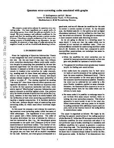
Figure 3.1: The relationship between a quantum stabilizer code Q and a classical code C, where C ⊆ C ⊥ . n
only if Q is a K-dimensional subspace of Cq that has minimum distance d. An ((n, q k , d))q code is also called an [[n, k, d]]q code. One of these two notations will be used when needed. Due to the linearity of quantum mechanics, a quantum error-correcting code that can detect a set D of errors, can also detect all errors in the linear span of D. A code of minimum distance d can correct all errors of weight t = ⌊(d − 1)/2⌋ or less. Pure and Impure Codes. We say that a quantum code Q is pure to t if and only if its stabilizer group S does not contain non-scalar error operators of weight less than t. An [[n, k, d]]q quantum code is called pure if and only if it is pure to its minimum distance d. We will follow the same convention as in [34], that an [[n, 0, d]]q code is pure. Impure codes are also referred to as degenerate codes. Degenerate codes are of interest because they have the potential for passive error-correction and they are difficult to construct as we will explain later.
3.1.4
Encoding Quantum Codes
The Stabilizer S of a quantum code Q provides also a means for encoding quantum codes. The essential idea is to encode the information into the code space through a projector. For an ((n, K, d))q quantum code with stabilizer S, the projector P is defined as 1 X (3.7) P = E. |S| E∈S
It can be checked that P is an orthogonal projector onto a vector space Q. Further, we have K = dim Q = Tr P = q n /|S|.
(3.8)
The stabilizer allows us to derive encoded operators, so that we can operate directly on the encoded data instead of decoding and then operating on them. These operators are in CGn (S). See [70] and [83] for more details.
3.2
Deriving Quantum Codes from Self-orthogonal Classical Codes
In this section we show how stabilizer codes are related to classical codes (additive codes over Fq or over Fq2 ). The central idea behind this relation is the fact insofar as the detectability of an error is concerned the phase information is irrelevant. This means we can factor out the phase defining a map from Gn onto n F2n q and study the images of S and CGn (S). We will denote a classical code C ≤ Fq with K codewords and distance d by (n, K, d)q . If it is linear then we will also denote it by [n, k, d]q where k = logq K. We define P the Euclidean inner product of x, y ∈ Fnq as x · y = ni=1 xi yi . The dual code C ⊥ is the set of vectors in Fnq orthogonal to C i.e., C ⊥ = {x ∈ Fnq | x · c = 0 for all c ∈ C}. For more details on classical codes see [88] or [130].
16
Chapter 3: Fundamentals of Quantum Block Codes
Constructing a quantum code Q reduces to constructing a self-orthogonal classical code C over Fq and F2q , see [41, 40, 34, 70, 74, 179, 177, 168]. This relationship is shown in Fig. 3.1. Fact 12 (CSS Code Construction). Let C1 and C2 denote two classical linear codes with parameters [n, k1 , d1 ]q and [n, k2 , d2 ]q such that C2⊥ ≤ C1 . Then there exists a [[n, k1 + k2 − n, d]]q stabilizer code with minimum distance d = min{wt(c) | c ∈ (C1 \ C2⊥ ) ∪ (C2 \ C1⊥ )} ≥ min{d1 , d2 }.
Also, we can construct quantum codes from classical codes that contain their duals or are self-orthogonal as follows: Fact 13. If C is a classical linear [n, k, d]q code containing its dual, C ⊥ ≤ C, then there exists a [[n, 2k−n, d]]q stabilizer code.
Fact 13 is particularly interesting because it helps us to construct a quantum code from a classical code and its dual. There have been many families of quantum codes based on binary classical codes, see [76, 75, 78, 98]. The theory has been generalized to finite fields, see [20, 53, 54, 71, 99, 152, 158, 165]. Recently, new bounds, encoding circuits, and new families have been investigated, see [16, 17, 55, 83, 53, 124, 158].
3.2.1
Codes over Fq .
If we associate with an element ω c X(a)Z(b) of Gn an element (a|b) of F2n q , then the group SZ(Gn ) is mapped to the additive code C = {(a|b) | ω c X(a)Z(b) ∈ SZ(Gn )} = SZ(Gn )/Z(Gn ).
(3.9)
To relate the images of the stabilizer and its centralizer, we need the notion of a trace-symplectic form of two vectors (a|b) and (a′ |b′ ) in F2n q , < (a|b) | (a′ |b′ ) >s = trq/p (b · a′ − b′ · a).
(3.10)
Let C ⊥s be the trace-symplectic dual of C defined as C ⊥s = {x ∈ F2n q |< x| c >s = 0 for all c ∈ C}.
(3.11)
The centralizer CGn (S) contains all elements of Gn that commute with each element of S; thus, by Lemma 11, CGn (S) is mapped onto the trace-symplectic dual code C ⊥s of the code C, C ⊥s = {(a|b) | ω c X(a)Z(b) ∈ CGn (S)}.
(3.12)
The next theorem illustrates this connection between classical codes and stabilizer codes and generalizes the well-known connection to symplectic codes [34, 69] of the binary case. Theorem 14. An ((n, K, d))q stabilizer code exists if and only if there exists an additive code C ≤ F2n q of size |C| = q n /K such that C ≤ C ⊥s and swt(C ⊥s \ C) = d if K > 1( and swt(C ⊥s ) = d if K = 1). Proof. See [20, 97] for the proof.
In 1996, Calderbank and Shor [35] and Steane [177] introduced the following construction of quantum codes. It is perhaps the simplest method to build quantum codes via classical codes over Fq . Lemma 15 (CSS Code Construction). Let C1 and C2 denote two classical linear codes with parameters [n, k1 , d1 ]q and [n, k2 , d2 ]q such that C2⊥ ≤ C1 . Then there exists a [[n, k1 + k2 − n, d]]q stabilizer code with minimum distance d = min{wt(c) | c ∈ (C1 \ C2⊥ ) ∪ (C2 \ C1⊥ )} that is pure to min{d1 , d2 }.
′ ′ Proof. Let C = C1⊥ × C2⊥ ≤ F2n q . Clearly C ≤ C2 × C1 . If (c1 | c2 ) ∈ C and (c1 | c2 ) ∈ C2 × C1 , then we ′ ′ ⊥s observe that tr(c2 · c1 − c2 · c1 ) = tr(0 − 0) = 0. Therefore, C ≤ C2 × C1 ≤ C . Since |C| = q 2n−k1 −k2 , |C ⊥s | = q 2n /|C| = q k1 +k2 = |C2 ×C1 |. Therefore, C ⊥s = C2 ×C1 . By Theorem 14 there exists an ((n, K, d))q quantum code with K = q n /|C| = q k1 +k2 −n . The claim about the minimum distance and purity of the code is obvious from the construction.
Corollary 16. If C is a classical linear [n, k, d]q code containing its dual, C ⊥ ≤ C, then there exists an [[n, 2k − n, ≥ d]]q stabilizer code that is pure to d.
We will use Lemma 15 and Corollary 16 to derive many families of quantum error-correcting codes based on BCH, RS, duadic, and projective geometry codes as shown in the following sections.
3.3. Bounds on Quantum Codes
3.2.2
17
Codes over Fq2 .
We can also extend the connection of the quantum codes and classical codes that are defined over Fq2 , especially as it allows us the use of codes over quadratic extension fields. The binary case was done in [34] and partial generalizations were done in [132, 99] and [152]. We provide a slightly alternative generalization using a trace-alternating form. Let (β, β q ) denote a normal basis of Fq2 over Fq . We define a trace-alternating form of two vectors v and w in Fnq2 by (v|w)a = trq/p
�
v · wq − v q · w β 2q − β 2
�
.
(3.13)
The argument of the trace is an element of Fq as it is invariant under the Galois automorphism x 7→ xq . n q Let φ : F2n q → Fq2 take (a|b) 7→ βa + β b. The map φ is isometric in the sense that the symplectic weight of (a|b) is equal to the Hamming weight of φ((a|b)). This map allows us to transform the tracesymplectic duality into trace-alternating duality. In particular it can be easily verified that if c, d ∈ F2n q , then < c, | d > s = (φ(c), |, φ(d))a. If D ≤ Fnq2 , then we denote its trace-alternating dual by D⊥a = {v ∈ Fnq2 | (v|w)a = 0 for all w ∈ D}. Now Theorem 14 can be reformulated as: Theorem 17. An ((n, K, d))q stabilizer code exists if and only if there exists an additive subcode D of Fnq2 of cardinality |D| = q n /K such that D ≤ D⊥a and wt(D⊥a \ D) = d if K > 1 (and wt(D⊥a ) = d if K = 1). Proof. From Theorem 14 we know that an ((n, K, d))q stabilizer code exists if and only if there exists a code n ⊥s C ≤ F2n , and swt(C ⊥s \ C) = d if K > 1 (and swt(C ⊥s ) = d if K = 1). q such that |C| = q /K, C ≤ C The theorem follows simply by applying the isometry φ. If we restrict our attention to linear codes over Fq2 , then the hermitian form is more useful. The hermitian inner product of two vectors x and y in Fnq2 is given by xq · y. From the definition of the trace-alternating form it is clear that if two vectors are orthogonal with respect to the hermitian form they are also orthogonal with respect to the trace-alternating form. Consequently, if D ≤ Fnq2 , then D⊥h ≤ D⊥a , where D⊥h = {v ∈ Fnq2 | v q · w = 0 for all w ∈ D}. Therefore, any self-orthogonal code with respect to the hermitian inner product is self-orthogonal with respect to the trace-alternating form. In general, the two dual spaces D⊥h and D⊥a are not the same. However, if D happens to be Fq2 -linear, then the two dual spaces coincide. Corollary 18. If there exists an Fq2 -linear [n, k, d]q2 code D such that D⊥h ≤ D, then there exists an [[n, 2k − n, ≥ d]]q quantum code that is pure to d. Proof. Let q = pm , p prime. If D is a k-dimensional subspace of Fnq2 , then D⊥h is a (n − k)-dimensional subspace of Fnq2 . We can also view D as a 2mk-dimensional subspace of F2mn , and D⊥a as a 2m(n − k)p 2mn ⊥h ⊥a ⊥a dimensional subspace of Fp . Since D ⊆D and the cardinalities of D and D⊥h are the same, we ⊥h ⊥a can conclude that D = D . The claim follows from Theorem 17. So it is sufficient to consider the hermitian form in case of Fq2 -linear codes. For additive codes (that are not linear) over Fq2 we have to use the rather inconvenient trace-alternating form. Finally, using the hermitian construction, we will derive many families of quantum error-correcting codes in the following sections.
3.3
Bounds on Quantum Codes
We need some bounds on the achievable minimum distance of a quantum stabilizer code. Perhaps the simplest one is the Knill-LaFlamme bound, also called the quantum Singleton bound. The binary version of the quantum Singleton bound was first proved by Knill and Laflamme in [106], see also [21, 19], and later generalized by Rains using weight enumerators in [152]. Theorem 19 (Quantum Singleton Bound). An ((n, K, d))q stabilizer code with K > 1 satisfies K ≤ q n−2d+2 .
(3.14)
18
Chapter 3: Fundamentals of Quantum Block Codes
All binary and nonbinary quantum codes obeys the quantum Singleton bound as shown in Theorem 19. In addition all pure and impure quantum codes satisfies this bound as well. Codes which meet the quantum Singleton bound are called quantum MDS codes. In [97], it was showed that these codes cannot be indefinitely long and the maximal length of a q-ary quantum MDS codes is upper bounded by 2q 2 −2. This could probably be tightened to q 2 + 2. It would be interesting to find quantum MDS codes of length greater than q 2 + 2 since it would disprove the MDS Conjecture for classical codes [88]. A related open question is regarding the construction of codes with lengths between q and q 2 − 1. At the moment there are no analytical methods for constructing a quantum MDS code of arbitrary length in this range (see [77] for some numerical results). Another important bound for quantum codes is the quantum Hamming bound. The quantum Hamming bound states (see [69, 55]) that: Theorem 20 (Quantum Hamming Bound). Any pure ((n, K, d))q stabilizer code satisfies ⌊(d−1)/2⌋ �
� n (q 2 − 1)i ≤ q n /K. i
X i=0
(3.15)
While the quantum Singleton bound holds for all quantum codes, it is not known if the quantum Hamming bound is of equal applicability. So far no degenerate quantum code has been found that beats this bound. Gottesman showed that impure binary quantum codes cannot beat the quantum Hamming bound [70]. In [21] Ashikhmin and Litsyn derived many bounds for quantum codes by extending a novel method originally introduced by Delsarte [47] for classical codes. Using this method they proved the binary versions of Theorem 20 and Theorem 19. We use this method to show that the Hamming bound holds for all double error-correcting quantum codes. See [97] for a similar result for single error-correcting codes. But first we need Theorem 21 and the Krawtchouk polynomial of degree j in the variable x, Kj (x) =
j X s=0
s
2
j−s
(−1) (q − 1)
� �� � x n−x . s j−s
(3.16)
Theorem 21. Let Q be an ((n, K, d))q stabilizer code of dimension K > 1. Suppose that S is a nonempty subset of {0, . . . , d − 1} and N = {0, . . . , n}. Let n X
fi Ki (x)
(3.17)
f (x) 1 max . q n x∈S fx
(3.18)
f (x) =
i=0
be a polynomial satisfying the conditions i) fx > 0 for all x in S, and fx ≥ 0 otherwise; ii) f (x) ≤ 0 for all x in N \ S. Then K≤ Proof. See [97]. We demonstrate usefulness of the previous theorem by showing that the quantum Hamming bound holds for impure nonbinary codes when d = 5. Lemma 22 (Quantum Hamming Bound). An ((n, K, 5))q stabilizer code with K > 1 satisfies � K ≤ q n (n(n − 1)(q 2 − 1)2 /2 + n(q 2 − 1) + 1).
(3.19)
3.4. Perfect Quantum Codes
19
Pe Pn Proof. Let f (x) = j=0 fj Kj (x), where fx = ( j=0 Kj (x))2 , S = {0, 1, . . . , 4} and N={0,1,. . . ,n}. Calculating f (x) and fx gives us f0
=
f1
=
f2
=
f3
=
f4
=
(1 + n(q 2 − 1) + n(n − 1)(q 2 − 1)2 /2)2 1 (n − 1)2 (n − 2)2 (q 2 − 1)4 4 1 ( (n − 3)(n − 2)(q 2 − 1)2 − (n − 2)(q 2 − 1))2 2 1 (1 − 2(n − 3)(q 2 − 1) + (n − 4)(n − 3)(q 2 − 1)2 )2 2 1 2 (3 − 3(n − 4)(q − 1) + (n − 5)(n − 4)(q 2 − 1)2 )2 2
and, f (0) = f (1) = f (2) = f (3) = f (4) =
1 q 2n (1 + n(q 2 − 1) + (n − 1)n(q 2 − 1)2 ) 2 q 2n (q 2 + 2(n − 1)(q 2 − 1) + (n − 1)(q 2 − 2)(q 2 − 1)) q 2n (4 + 4(q 2 − 2) + (q 2 − 2)2 + 2(n − 2)(q 2 − 1)) q 2n (6 + 6(q 2 − 2)) 6q 2n .
Clearly fx > 0 for all x ∈ S . Also, f (x) ≤ 0 for all x ∈ N \S since the binomial coefficients for negative values are zero. The Hamming bound is given by K ≤ q −n max s∈S
f (x) fx
(3.20)
So, there are four different comparisons where f (0)/f0 ≥ f (x)/fx , for x = 1, 2, 3, 4. We find a lower bound for n that holds for all values of q. For n ≥ 7 it follows that max{f (0)/f0 , f (1)/f1 , f (2)/f2 , f (3)/f3 , f (4)/f4 } = f (0)/f0
(3.21)
The detailed prove of Lemma 22 can be found in [8]. While the above method is a general method to prove Hamming bound for impure quantum codes, the number of terms increases with a large minimum distance. It becomes difficult to find the true bound using this method. However, one can derive more consequences from Theorem 21; see, for instance, [21, 19, 123, 134].
3.4
Perfect Quantum Codes
A quantum code that meets the quantum Hamming bound with equality is known as a perfect quantum code. In fact the famous [[5, 1, 3]]2 code [119] is one such. We will show that there do not exist any pure perfect quantum codes other than the ones mentioned in the following theorem. It is actually a very easy result and follows from known results on classical perfect codes, but we had not seen this result earlier in the literature. Theorem 23. There do not exist any pure perfect quantum codes with distance greater than 3. Proof. Assume that Q is a pure perfect quantum code with the parameters ((n, K, d))q . Since it meets the quantum Hamming bound we have ⌊(d−1)/2⌋ �
X j=0
� n (q 2 − 1)j = q n /K. j
(3.22)
By Theorem 17 the associated classical code C is such that C ⊥a ≤ C ≤ Fnq2 and has parameters (n, q n K, d)q2 . Its distance is d because the quantum code is pure. Now C obeys the classical Hamming bound (see [88,
20
Chapter 3: Fundamentals of Quantum Block Codes
Theorem 1.12.1] or any textbook on classical codes). Hence q 2n . |C| = q n K ≤ P⌊(d−1)/2⌋ n� 2 j j=0 j (q − 1)
(3.23)
Substituting the value of K we see that this implies that C is a perfect classical code. But the only perfect classical codes with distance greater than 3 are the Golay codes and the repetition codes [88]. The perfect Golay codes are over F2 and F3 not over a quadratic extension field as C is required to be. The repetition codes are of dimension 1 and cannot contain their duals as C is required to contain. Hence C cannot be anyone of them. Therefore, there are no pure quantum codes of distance greater than 3 that meet the quantum Hamming bound. Since it is not known if the quantum Hamming bound holds for nonbinary degenerate quantum codes with distance d > 5, it would be interesting to find degenerate quantum codes that either meet or beat the quantum Hamming bound [8]. This is obviously a challenging open research problem.
CHAPTER
4
Quantum BCH Codes
An attractive feature of BCH codes is that one can infer valuable information from their design parameters (length, size of the finite field, and designed distance), such as bounds on the minimum distance and dimension of the code. In this chapter, we show that one can also deduce from the design parameters whether or not a primitive, narrow-sense BCH contains its Euclidean or Hermitian dual code. This information is invaluable in the construction of quantum BCH codes. A new proof is provided for the dimension of BCH codes with small designed distance, and simple bounds on the minimum distance of such codes and their duals are derived as a consequence. These results allow us to derive the parameters of two families of primitive quantum BCH codes as a function of their design parameters. This chapter is based on a joint work with P.K. Sarvepalli and A. Klappenecker and it was presented in [13, 16].
4.1
BCH Codes
The Bose-Chaudhuri-Hocquenghem (BCH) codes [29, 30, 68, 85] are a well-studied class of cyclic codes that have found numerous applications in classical and more recently in quantum information processing. Recall that a cyclic code of length n over a finite field Fq with q elements, and gcd(n, q) = 1, is called a BCH code with designed distance δ if its generator polynomial is of the form Y g(x) = (x − αz ), Z = Cb ∪ · · · ∪ Cb+δ−2 , z∈Z
where Cx = {xq k mod n | k ∈ Z, k ≥ 0 } denotes the q-ary cyclotomic coset of x modulo n, α is a primitive element of Fqm , and m = ordn (q) is the multiplicative order of q modulo n. Such a code is called primitive if n = q m − 1, and narrow-sense if b = 1. An attractive feature of a (narrow-sense) BCH code is that one can derive many structural properties of the code from the knowledge of the parameters n, q, and δ alone. Perhaps the most well-known facts are that such a code has minimum distance d ≥ δ and dimension k ≥ n − (δ − 1) ordn (q). In this chapter, we will show that a necessary condition for a narrow-sense BCH code which contains its Euclidean dual code is that its designed distance δ = O(qn1/2 ). We also derive a sufficient condition for dual containing BCH codes. Moreover, if the codes are primitive, these conditions are same. These results allow us to derive families of quantum stabilizer codes. Along the way, we find new results concerning the minimum distance and dimension of classical BCH codes. To put our results into context, we give a brief overview of related work in quantum BCH codes. This chapter was motivated by problems concerning quantum BCH codes; specifically, our goal was to derive the parameters of the quantum codes as a function of the design parameters. Examples of certain binary quantum BCH codes have been given by many authors, see, for example, [34, 76, 75, 177]. Steane [179] gave a simple criterion to decide when a binary narrow-sense primitive BCH code contains its dual, given the 21
22
Chapter 4: Quantum BCH Codes
design distance and the length of the code. We generalize Steane’s result in various ways, in particular, to narrow-sense (not necessarily primitive) BCH codes over arbitrary finite fields with respect to Euclidean and Hermitian duality. These results allow one to derive quantum BCH codes; however, it remains to determine the dimension, purity, and minimum distance of such quantum codes. The dimension of a classical BCH code can be bounded by many different standard methods, see [27, 88, 130] and the references therein. An upper bound on the dimension was given by Shparlinski [170], see also [110, Chapter 17]. More recently, the dimension of primitive narrow-sense BCH codes of designed distance δ < q ⌈m/2⌉ + 1 was apparently determined by Yue and Hu [191], according to reference [190]. We generalize their result and determine the dimension of narrow-sense BCH codes for a certain range of designed distances. As desired, this result allows us to explicitly obtain the dimension of the quantum codes without computation of cyclotomic cosets. The purity and minimum distance of a quantum BCH code depend on the minimum distance and dual distance of the associated classical code. In general, it is a difficult problem to determine the true minimum distance of BCH codes, see [37]. A lower bound on the dual distance can be given by the CarlitzUchiyama-type bounds when the number of field elements is prime, see, for example, [130, page 280] and [183]. Many authors have determined the true minimum distance of BCH codes in special cases, see, for instance, [143],[190]. We refer to such a code as a BCH(n, q; δ) code, and call Z the defining set of the code. The basic properties of these classical codes are discussed, for example, in the books [88, 93, 130]. Given a classical BCH code, we can use one of the following well-known constructions to derive a quantum stabilizer code: 1. If there exists a classical linear [n, k, d]q code C such that C ⊥ ⊆ C, then there exists an [[n, 2k − n, ≥ d]]q stabilizer code that is pure to d. If the minimum distance of C ⊥ exceeds d, then the quantum code is pure and has minimum distance d. 2. If there exists a classical linear [n, k, d]q2 code D such that D⊥h ⊆ D, then there exists an [[n, 2k −n, ≥ d]]q stabilizer code that is pure to d. If the minimum distance of D⊥h exceeds d, then the quantum code is pure and has minimum distance d. The orthogonality relations are defined in the Notations at the end of this section. Examples of certain binary quantum BCH codes have been given in [34, 76, 77, 177]. Our goal is to derive the parameters of the quantum stabilizer code as a function of their design parameters n, q, and δ of the associated primitive, narrow-sense BCH code C. This entails the following tasks: a) Determine the design parameters for which C ⊥ ⊆ C; b) determine the dimension of C; c) bound the minimum distance of C and C ⊥ . In case q is a perfect square, we would also like to answer the Hermitian versions of questions a) and c): a’) Determine the design parameters for which C ⊥h ⊆ C; c’) bound the minimum distance of C and C ⊥h . To put our work into perspective, we sketch our results and give a brief overview of related work. Let C be a primitive, narrow-sense BCH code C of length n = q m − 1, m ≥ 2, over Fq with designed distance δ. To answer question a), we prove in Theorem 34 that C ⊥ ⊆ C holds if and only if δ ≤ q ⌈m/2⌉ − 1 − (q − 2)[m odd]. The significance of this result is that allows one to identify all BCH codes that can be used in the quantum code construction 1). Fortunately, this question can be answered now without computations. Steane proved in [179] the special case q = 2, which is easier to show, since in this case there is no difference between even and odd m. In Theorem 36, we answer question a’) and show that C ⊥h ⊆ C if and only if δ ≤ q (m+[m even])/2 − 1 − (q − 2)[m even], where we assume that q is a perfect square. This result allows us to determine all primitive, narrow-sense BCH codes that can be used in construction 2). We are not aware of any prior work concerning the Hermitian case.
4.2. Dimension and Minimum Distance
23
In the binary case, an answer to question b) was given by MacWilliams and Sloane [130, Chapter 9, Corollary 8]. Apparently, Yue and Hu answered question b) in the case of small designed distances [191]. We give a new proof of this result in Theorem 26 and show that the dimension k = n − m ⌈(δ − 1)(1 − 1/q)⌉ for δ in the range 2 ≤ δ < q ⌈m/2⌉ + 1. As a consequence of our answer to b), we obtain the dimensions of the quantum codes in constructions 1) and 2). Finding the true minimum distance of BCH codes is an open problem for which a complete answer seems out of reach, see [37]. As a simple consequence of our answer to b), we obtain better bounds on the minimum distance for some BCH codes, and we derive simple bounds on the (Hermitian) dual distance of BCH codes with small designed distance, which partly answers c) and c’). In Section 4.5, all these results are used to derive two families of quantum BCH codes. Impatient readers should now browse this section to get the bigger picture. Theorem 217 yields the result that one obtains using construction 1). Cohen, Encheva, and Litsyn derived in [42] the special case q = 2 of our theorem by combining the results of Steane, and MacWilliams and Sloane that we have mentioned already. The result of construction 2) is given in Theorem 38. Notations. We denote the ring of integers by Z and a finite field with q elements by Fq . We follow Knuth and attribute to [P (k)] the value 1 if the property P (k) of the integer k is true, and 0 otherwise. For instance, we have [k even] = k − 1 mod 2, but the left hand side seems more readable. If x and y are vectors in Fnq , then we write x ⊥ y if and only if x · y = 0. Similarly, if x and y are vectors in Fnq2 , then we write x ⊥h y if and only if xq · y = 0.
4.2
Dimension and Minimum Distance
In this section we determine the dimension of primitive, narrow-sense BCH codes of length n with small designed distance. Furthermore, we derive bounds on the minimum distance of such codes and their duals.
4.2.1
Dimension
First, we make some simple observations about cyclotomic cosets that are essential in our proof. Lemma 24. If q be a power of a prime, m a positive integer and n = q m − 1, then all q-ary cyclotomic cosets Cx = {xq ℓ mod n | ℓ ∈ Z} with x in the range 1 ≤ x < q ⌈m/2⌉ + 1 have cardinality |Cx | = m. Proof. Seeking a contradiction, we assume that |Cx | < m. If m = 1, then Cx would have to be the empty set, which is impossible. If m > 1, then |Cx | < m implies that there must exist an integer j in the range 1 ≤ j < m such that j divides m and xq j ≡ x mod n. In other words, q m − 1 divides x(q j − 1); hence, x ≥ (q m − 1)/(q j − 1). If m is even, then j ≤ m/2; thus, x ≥ q m/2 + 1. If m is odd, then j ≤ m/3 and it follows that x ≥ (q m − 1)/(q m/3 − 1), and it is easy to see that the latter term is larger than q ⌈m/2⌉ + 1. In both cases this contradicts our assumption that 1 ≤ x ≤ q ⌈m/2⌉ ; hence |Cx | = m. Lemma 25. Let q be a power of a prime, m a positive integer, and n = q m − 1. Let x and y be integers in the range 1 ≤ x, y < q ⌈m/2⌉ + 1 such that x, y 6≡ 0 mod q. If x 6= y, then the q-ary cosets of x and y modulo n are disjoint, i.e., Cx 6= Cy . Proof. Seeking a contradiction, we assume that Cx = Cy . This assumption implies that y ≡ xq ℓ mod n for some integer ℓ in the range 1 ≤ ℓ < m. If xq ℓ < n, then xq ℓ ≡ 0 mod q; this contradicts our assumption y 6≡ 0 mod q, so we must have xq ℓ ≥ n. It follows from the range of x that ℓ must be at least ⌊m/2⌋. If ℓ = ⌊m/2⌋, then we cannot find an admissible x within the given range such that y ≡ xq ⌊m/2⌋ mod n. Indeed, it follows from the inequality xq ⌊m/2⌋ ≥ n that x ≥ q ⌈m/2⌉ , so x must equal q ⌈m/2⌉ , but that contradicts x 6≡ 0 mod q. Therefore, ℓ must exceed ⌊m/2⌋. Let us write x as a q-ary number x = x0 +x1 q+· · ·+xm−1 q m−1 , with 0 ≤ xi < q. Note that x0 6= 0 because x 6≡ 0 mod q. If ⌊m/2⌋ < ℓ < m, then xq ℓ is congruent to y0 = xm−ℓ +· · ·+xm−1 q ℓ−1 +x0 q ℓ +· · ·+xm−ℓ−1 q m−1 modulo n. We observe that y0 ≥ x0 q ℓ ≥ q ⌈m/2⌉ . Since y 6≡ 0 mod q, it follows that y = y0 ≥ q ⌈m/2⌉ + 1, contradicting the assumed range of y.
24
Chapter 4: Quantum BCH Codes
The previous two observations about cyclotomic cosets allow us to derive a closed form for the dimension of a primitive BCH code. This result generalizes binary case [130, Corollary 9.8, page 263]. See also [182] which gives estimates on the dimension of BCH codes among other things. Theorem 26. A primitive, narrow-sense BCH code of length q m − 1 over Fq with designed distance δ in the range 2 ≤ δ ≤ q ⌈m/2⌉ + 1 has dimension k = q m − 1 − m⌈(δ − 1)(1 − 1/q)⌉.
(4.1)
Proof. The defining set of the code is of the form Z = C1 ∪ C2 · · · ∪ Cδ−1 , a union of at most δ − 1 consecutive cyclotomic cosets. However, when 1 ≤ x ≤ δ − 1 is a multiple of q, then Cx/q = Cx . Therefore, the number of cosets is reduced by ⌊(δ − 1)/q⌋. By Lemma 25, if x, y 6≡ 0 mod q and x 6= y, then the cosets Cx and Cy are disjoint. Thus, Z is the union of (δ − 1) − ⌊(δ − 1)/q⌋ = ⌈(δ − 1)(1 − 1/q)⌉ distinct cyclotomic cosets. By Lemma 24 all these cosets have cardinality m. Therefore, the degree of the generator polynomial is m⌈(δ − 1)(1 − 1/q)⌉, which proves our claim about the dimension of the code. If we exceed the range of the designed distance in the hypothesis of the previous theorem, then our dimension formula (4.1) is no longer valid, as our next example illustrates. Example 27. Consider a primitive, narrow-sense BCH code of length n = 42 − 1 = 15 over F4 . If we choose the designed distance δ = 6 > 41 + 1, then the resulting code has dimension k = 8, because the defining set Z is given by Z = C1 ∪ C2 ∪ · · · ∪ C5 = {1, 4} ∪ {2, 8} ∪ {3, 12} ∪ {5}.
The dimension formula (4.1) yields 42 − 1 − 2⌈(6 − 1)(1 − 1/4)⌉ = 7, so the formula does not extend beyond the range of designed distances given in Theorem 26.
4.2.2
Distance Bounds
The true minimum distance dmin of a primitive BCH code over Fq with designed distance δ is bounded by δ ≤ dmin ≤ qδ − 1, see [130, p. 261]. If we apply the Farr bound (essentially the sphere packing bound) using the dimension given in Theorem 26, then we obtain: Corollary 28. If C is primitive, narrow-sense BCH code of length q m − 1 over Fq with designed distance δ in the range 2 ≤ δ ≤ q ⌈m/2⌉ + 1 such that ⌊(δ+1)/2⌋ � m X
q
i=0
� −1 (q − 1)i > q m⌈(δ−1)(1−1/q)⌉ , i
(4.2)
then C has minimum distance d = δ or δ + 1; if, furthermore, δ ≡ 0 mod q, then d = δ + 1. Proof. Seeking a contradiction, we assume that the minimum distance d of the code satisfies d ≥ δ + 2. We know from Theorem 26 that the dimension of the code is k = q m − 1 − m⌈(δ − 1)(1 − 1/q)⌉. If we substitute this value of k into the sphere-packing bound qk
⌊(d−1)/2⌋ � m X
q
i=0
� −1 (q − 1)i ≤ q n , i
then we obtain ⌊(δ+1)/2⌋ � m X
q
i=0
� � ⌊(d−1)/2⌋ � m X q −1 −1 (q − 1)i (q − 1)i ≤ i i i=0 ≤ q m⌈(δ−1)(1−1/q)⌉ ,
but this contradicts condition (4.2); hence, δ ≤ d ≤ δ + 1. If δ ≡ 0 mod q, then the cyclotomic coset Cδ is contained in the defining set Z of the code because Cδ = Cδ/q . Thus, the BCH bound implies that the minimum distance must be at least δ + 1.
4.3. Euclidean Dual Codes
25
Corollary 29. A primitive, narrow sense BCH code of length n = q m − 1 over Fq with designed distance δ in the range 2 ≤ δ ≤ q ⌈m/2⌉ + 1 that satisfies n
34 . This means that condition (4.2) holds, then by Corollary 28, the i code of length 8 and designed distance δ = 4 has a minimum distance dmin = 4. To verify that, let us construct a primitive narrow-sense BCH code with length n = 8 and designed distance δ = 4. We have k = q m − 1 − m⌈2t(1 − 1/q)⌉ = 4 and the generator polynomial is g(x) = 2 + x + x3 + x4 and the parity check polynomial is h(x) = 1 + x + x2 + 2x3 + x4 . So, hR (x) = 1 + 2x + x2 + x3 + x4 and the parity check matrix is 1 1 1 2 1 0 0 0 0 1 1 1 2 1 0 0 H= 0 0 1 1 1 2 1 0 0 0 0 1 1 1 2 1 by subtracting columns 4 and 5 then add the result to columns 1 and 2, we found that the min distance for this matrix H is 4 that verifies our claim in Corollary 28 where 2t + 1 ≡ 0 mod 3.
Lemma 31. Suppose that C is a primitive, narrow-sense BCH code of length n = q m − 1 over Fq with designed distance 2 ≤ δ ≤ δmax = q ⌈m/2⌉ − 1 − (q − 2)[m odd]), then the dual distance d⊥ ≥ δmax + 1. Proof. Let N = {0, 1, . . . , n − 1} and Zδ be the defining set of C. We know that Zδmax ⊇ Zδ ⊃ {1, . . . , δ − 1}. Therefore N \ Zδmax ⊆ N \ Zδ . Further, we know that Z ∩ Z −1 = ∅ if 2 ≤ δ ≤ δmax from Lemma 33 and ⊆ N \ Zδmax ⊆ N \ Zδ . Theorem 34. Therefore, Zδ−1 max Let Tδ be the defining set of the dual code. Then Tδ = (N \ Zδ )−1 ⊇ Zδmax . Moreover {0} ∈ N \ Zδ and therefore Tδ . Thus there are at l east δmax consecutive roots in Tδ . Thus the dual distance d⊥ ≥ δmax + 1. Lemma 32. Suppose that C is a primitive, narrow-sense BCH code of length n = q 2m − 1 over Fq2 with designed distance 2 ≤ δ ≤ δmax = q m+[m even] − 1 − (q 2 − 2)[m even]), then the dual distance d⊥ ≥ δmax + 1. Proof. The proof is analogous to the one of Lemma 31; just keep in mind that the defining set Zδ is invariant under multiplication by q 2 modulo n.
4.3
Euclidean Dual Codes
Recall that the Euclidean dual code C ⊥ of a code C ⊆ Fnq is given by C ⊥ = {y ∈ Fnq | x · y = 0 for all x ∈ C}. Steane showed in [179] that a primitive binary BCH code of length 2m − 1 contains its dual if and only if its designed distance δ satisfies δ ≤ 2⌈m/2⌉ − 1. In this section we derive a similar condition for nonbinary BCH codes. Lemma 33. Suppose that gcd(n, q) = 1. A cyclic code of length n over Fq with defining set Z contains its Euclidean dual code if and only if Z ∩ Z −1 = ∅, where Z −1 denotes the set Z −1 = {−z mod n | z ∈ Z}. Proof. See, for instance, [88, Theorem 4.4.11].
26
Chapter 4: Quantum BCH Codes
Theorem 34. A primitive, narrow-sense BCH code of length q m − 1, with m ≥ 2, over the finite field Fq contains its dual code if and only if its designed distance δ satisfies δ ≤ δmax = q ⌈m/2⌉ − 1 − (q − 2)[m odd]. Proof. Let n = q m − 1. The defining set Z of a primitive, narrow-sense BCH code C of designed distance δ is given by Z = C1 ∪ C2 · · · ∪ Cδ−1 , where Cx = {xq j mod n | j ∈ Z}. 1. We will show that the code C cannot contain its dual code if the designed distance δ > δmax . Seeking a contradiction, we assume that the defining set Z contains the set {1, . . . , s}, where s = δmax . By Lemma 33, it suffices to show that Z ∩ Z −1 is not empty. If m is even, then s = q m/2 − 1, and Z −1 contains the element −sq m/2 ≡ q m/2 − 1 ≡ s mod n, which means that Z ∩ Z −1 6= ∅; contradiction. If m is odd, then s = q (m+1)/2 − q + 1, and the element given by −sq (m−1)/2 ≡ q (m+1)/2 − q (m−1)/2 − 1 mod n is contained in Z −1 . Since this element is less than s for m ≥ 3, it is contained in Z, so Z ∩ Z −1 6= ∅; contradiction. Combining these two cases, we can conclude that δ ≤ q ⌈m/2⌉ − 1 − (q − 2)[m is odd] for m ≥ 2. 2. For the converse, we prove that if δ ≤ δmax , then Z ∩ Z −1 = ∅, which implies C ⊥ ⊆ C by Lemma 33. It suffices to show that min C−x ≥ δmax for any coset Cx in Z. Since 1 ≤ x < δmax ≤ q ⌈m/2⌉ − 1, we can write x as a q-ary integer of the form x = x0 + x1 q + · · · + xm−1P q m−1 with 0 ≤ xi < q, and xi = 0 for m−1 m−1 i ≥ ⌈m/2⌉. If y¯ = n − x, then y¯ = y¯0 + y¯1 q + · · · + y¯m−1 q = i=0 (q − 1 − xi )q i . Set y = min C−x . We note that y is a conjugate of y¯. Thus, the digits of y are obtained by cyclically shifting the digits of y¯. 3a) First we consider the case when m is even. Then the q-ary expansion of x has at least m/2 zero digits. P Therefore, at least m/2 of the y¯i are equal to q − 1. Thus, y ≥ m/2−1 (q − 1)q i = q m/2 − 1 = δmax . i=0
3b) If m is odd, then as 1 ≤ x < q (m+1)/2 −q +1, we have m > 1 and y¯ = y¯0 + y¯1 q +· · ·+(¯ y(m−1)/2 )q (m−1)/2 + (m+1)/2 m−1 (q − 1)q + · · · + (q − 1)q . For 0 ≤ j ≤ (m − 1)/2, we observe that xq j < n, and since j j j j y¯q ≡ −xq mod n, y¯q = n − xq ≥ q m − 1 − (q (m+1)/2 − q)q (m−1)/2 = q (m+1)/2 − 1 ≥ δmax . For (m + 1)/2 ≤ j ≤ m − 1, we find that y¯q j mod n = y¯m−j + · · · + y¯(m−1)/2 q j−(m+1)/2
+ (q − 1)q j−(m−1)/2 + · · · + (q − 1)q j−1 + y¯0 q j + · · · + y¯m−j−1 q m−1 ,
≥ (q (m−1)/2 − 1)q j−(m−1)/2 + y¯0 + · · ·
+ y¯(m−1)/2 ,
≥ q (m+1)/2 − q + 1 = δmax , where y¯0 + · · · + y¯(m−1)/2 ≥ 1 because x < q (m+1)/2 − q + 1. Hence y = min{¯ yq j | j ∈ Z} ≥ δmax when m is odd. Therefore a primitive BCH code contains its dual if and only if δ ≤ δmax , for m ≥ 2.
4.4
Hermitian Dual Codes
If the cardinality of the field is a perfect square, then we can define another type of orthogonality relation for codes. Recall that if the code C is a subspace of the vector space Fnq2 , then its Hermitian dual code C ⊥h is given by C ⊥h = {y ∈ Fnq2 | y q · x = 0 for all x ∈ C}, where y q = (y1q , . . . , ynq ) denotes the conjugate of the vector y = (y1 , . . . , yn ). The goal of this section is to establish when a primitive, narrow-sense BCH code contains its Hermitian dual code. Lemma 35. Assume that gcd(n, q) = 1. A cyclic code of length n over Fq2 with defining set Z contains its Hermitian dual code if and only if Z ∩ Z −q = ∅, where Z −q = {−qz mod n | z ∈ Z}.
4.5. Families of Quantum BCH Codes
27
Q Proof. Let N = {0, 1, . . . , n − 1}. If g(z) = x∈Z (z − αx ) is the generator polynomial of a cyclic code C, Q then h† (z) = x∈N \Z (z − α−qx ) is the generator polynomial of C ⊥h . Thus, C ⊥h ⊆ C if and only if g(z) divides h† (z). The latter condition is equivalent to Z ⊆ {−qx | x ∈ N \ Z}, which can also be expressed as Z ∩ Z −q = ∅. Theorem 36. A primitive, narrow-sense BCH code of length q 2m − 1 over Fq2 , where m 6= 2, contains its Hermitian dual code if and only if its designed distance δ satisfies δ ≤ δmax = q m+[m even] − 1 − (q 2 − 2)[m even]. Proof. Let n = q 2m − 1. Recall that the defining set Z of a primitive, narrow-sense BCH code C over the finite field Fq2 with designed distance δ is given by Z = C1 ∪ · · · ∪ Cδ−1 with Cx = {xq 2j mod n | j ∈ Z}. 1. We will show that the code C cannot contain its Hermitian dual code if the designed distance δ > δmax . Seeking a contradiction, we assume that the defining set Z contains {1, . . . , s}, where s = δmax . By Lemma 35, it suffices to show that Z ∩ Z −q is not empty. If m is odd, then s = q m − 1. Notice that n − qsq 2(m−1)/2 = q m − 1 = s, which means that s ∈ Z ∩ Z −q , and this contradicts our assumption that this set is empty. If m is even, then s = q m+1 − q 2 + 1. We note that n − qsq m−2 = q m+1 − q m−1 − 1 < s = q m+1 − q 2 + 1, for m > 2. It follows that q m+1 − q m−1 − 1 ∈ Z ∩ Z −q , contradicting our assumption that this set is empty. Combining the two cases, we can conclude that s must be smaller than the value q m+[m even] − 1 − (q 2 − 2)[m even]. 2. For the converse, we show that if δ < δmax , then Z ∩ Z −q = ∅, which implies C ⊥h ⊆ C thanks to Lemma 35. It suffices to show that min{n − qCx } ≥ δmax or, equivalently, that max qCx ≤ n − δmax holds for 1 ≤ x ≤ δ − 1. 3. If m is odd, then the q-ary expansion of x is of the form x = x0 + x1 q + · · · + xm−1 q m−1 , with xi = 0, for m ≤ i ≤ 2m − 1 as x < q m − 1. So at least m of the xi are equal to zero, which implies max qCx < q 2m − 1 − (q m − 1) = n − δmax . 4. Let m be even and qxq 2j be the q 2 -ary conjugates of qx. Since x < q m+1 −q 2 +1, x = x0 +x1 q +· · ·+xm q m and at least one of the xi ≤ q − 2. If 0 ≤ 2j ≤ m − 2, then qxq 2j ≤ q(q m+1 − q 2 )q m−2 = q 2m − q m+1 = n−q m+1 +1 < n−δmax. If 2j = m, then qxq m = xm−1 +xm q +0.q 2 +· · ·+0.q m +x0 q m+1 · · ·+xm−2 q 2m−1 . We note that there occurs a consecutive string of m − 1 zeros and because one of the xi ≤ q − 2, we have qxq 2j < n − q 2 (q m−1 − 1) − 1 ≤ n − δmax . For m + 2 ≤ 2j ≤ 2m − 2, we see that qxq 2j < n − q 4 (q m−1 − 1) < n − δmax . Thus we can conclude that the primitive BCH codes contain their Hermitian duals when δ ≤ q m+[m even] − 1 − (q 2 − 2)[m even].
4.5
Families of Quantum BCH Codes
We use the results of the previous sections to prove the existence of quantum stabilizer codes. We use the CSS construction as shown in the previous Chapter. Theorem 37. If q is a power of a prime, and m and δ are integers such that m ≥ 2 and 2 ≤ δ ≤ δmax = q ⌈m/2⌉ − 1 − (q − 2)[m odd], then there exists a quantum stabilizer code Q with parameters [[q m − 1, q m − 1 − 2m⌈(δ − 1)(1 − 1/q)⌉, dQ ≥ δ]]q that is pure up to δ. If BCH(n, q; δ) has true minimum distance d, and d ≤ δmax , then Q is a pure quantum code with minimum distance dQ = d. Proof. Theorem 26 and 34 imply that there exists a classical BCH code with parameters [q m − 1, q m − 1 − m⌈(δ − 1)(1 − 1/q)⌉, ≥ δ]q which contains its dual code. An [n, k, d]q code that contains its dual code implies the existence of the quantum code with parameters [[n, 2k − n, ≥ d]]q by the CSS construction, see [77], [76]. By Lemma 31, the dual distance exceeds δmax ; the statement about the purity and minimum distance is an immediate consequence.
28
Chapter 4: Quantum BCH Codes
Theorem 38. If q is a power of a prime, m is a positive integer, and δ is an integer in the range 2 ≤ δ ≤ δmax = q m+[m even] − 1 − (q 2 − 2)[m even], then there exists a quantum code Q with parameters [[q 2m − 1, q 2m − 1 − 2m⌈(δ − 1)(1 − 1/q 2 )⌉, dQ ≥ δ]]q that is pure up to δ. If BCH(n, q 2 ; δ) has true minimum distance d, with d < δmax , then Q is a pure quantum code of minimum distance dQ = d. Proof. It follows from Theorems 26 and 36 that there exists a primitive, narrow-sense [q 2m − 1, q 2m − 1 − m⌈(δ − 1)(1 − 1/q 2 )⌉, ≥ δ]q2 BCH code that contains its Hermitian dual code. Recall that if a classical [n, k, d]q2 code C exists that contains its Hermitian dual code, then there exists an [[n, 2k − n, ≥ d]]q quantum code that is pure up to d, see [20]; this proves our claim. By Lemma 32, the Hermitian dual distance exceeds δmax , which implies the last statement of the claim.
4.6
Quantum BCH from Self-orthogonal Product Codes
It has been shown that product codes have a special interest because they have simple decoding algorithms and high bit rates. Furthermore, the Quantum BCH codes have much higher rates than the corresponding classical product codes. We apply an important result by Grassl [80, Theorem 5-8 ] in quantum block codes. Let Ci = [ni , ki , di ]q be a linear code over finite field Fq with generator matrix Gi for i ∈ {1, 2}. Then the linear code C = [n1 n2 , k1 k2 , d1 d2 ]q is the product code of C1 ⊗ C2 with generator matrix G = G1 ⊗ G2 , see [59, 80, 139]. ⊥ ⊥ Lemma 39. Let CE ⊆ CE and CH ⊆ CH denote two codes which are self-orthogonal with respect to the Euclidean and Hermitian inner products, respectively. Also, Let C and D denote arbitrary linear codes over Fq and Fq2 , respectively. Then C ⊗ CE and D ⊗ CH are Euclidean and Hermitian self-orthogonal codes, respectively. Furthermore, the minimum distance of the dual of the product code C ⊗ CE (D ⊗ CH ) cannot exceed the minimum distance of the dual distance of C(D) and the dual distance of CE (CH ).
Proof. See [80, Theorem 7, Corollary 6 ]. We can explicitly determine dimension of the new self-orthogonal product code if we know dimension of the original two self-orthogonal codes. Therefore, we apply our previous result in dimension of BCH codes as shown in section 2 into Lemmas 40 and 41. Lemma 40. Let Ci be a primitive narrow-sense BCH code with length ni = q mi − 1 and designed distance 2 ≤ δi ≤ q ⌈mi /2⌉ − 1 − (q − 2)[mi odd] over finite field Fq for i ∈ {1, 2}. Then the product code C1 ⊗ C2⊥ = [n1 n2 , k1 (n2 − k2 ), ≥ δ1 wt(C2⊥ )]q is self-orthogonal and its Euclidean dual code is (C1 ⊗ C2⊥ )⊥ = [n1 n2 , n1 n2 − k1 (n2 − k2 ), ≥ min(wt(C1⊥ ), δ2 )]q where ki = q mi − 1 − mi ⌈(δi − 1)(1 − 1/q)⌉ and wt(Ci⊥ ) ≥ δi .
Proof. We know that if 2 ≤ δ2 ≤ q m/2 −1, then C2 contains its Euclidean dual as shown in Theorem 34. From [80, Theorem 5] and Lemma 39, we conclude that the product code C1 ⊗ C2⊥ is Euclidean self-orthogonal. Lemma 41. Let C1 = [n, k, d] be a primitive narrow-sense BCH code with length n = q m − 1 and designed distance 2 ≤ δ ≤ q m/2 − 1 over Fq . Furthermore, let C2 = [q − 1, q − δ2 , δ2 ] be a self-orthogonal Reed-Solomon code. Then the product code C1 ⊗ C2 = [(q − 1)n, k(q − δ2 ), ≥ δ1 δ2 ]q is self-orthogonal with parameters
(C1 ⊗ C2 )⊥ = [(q − 1)n, (q − 1)n − k(q − δ2 ), ≥ min(wt(C1⊥ ), q − δ2 )]q
where k = q m − 1 − m⌈(δ1 − 1)(1 − 1/q)⌉ and wt(C1⊥ ) ≥ δ1 .
4.7. Conclusions and Discussion
29
Proof. Since C2 is a self-orthogonal code, then the dual code C2⊥ has minimum distance q − δ2 and dimension δ2 − 1. From [80, Theorem 5] and Lemma 39, we conclude that C1 ⊗ C2 is self-orthogonal. The dual distance of (C1 ⊗ C2 )⊥ comes from lemma 39 such that the dual distance of C2⊥ is wt(C2⊥ ) = q − δ2 . Now, we generalize the previous two lemmas to any arbitrary primitive BCH codes. Lemma 42. Let Ci be a primitive BCH code with length ni = q mi − 1 and designed distance 2 ≤ δi ≤ q ⌈mi /2⌉ − 1 − (q − 2)[mi odd] over Fq for i ∈ {1, 2}. Then the product code C1 ⊗ C2 = [n1 n2 , k1 k2 , ≥ δ1 δ2 ]q is self-orthogonal with parameters C1⊥ ⊗ C2⊥ = [n1 n2 , n1 n2 − k1 k2 , ≥ min(δ1⊥ , δ2⊥ )]q where ki = qim − 1 − mi ⌈(δi − 1)(1 − 1/q)⌉ and δi⊥ ≥ δi . Proof. Direct conclusion and similar proof as Lemma 40. Note: Lemmas 41 and 40 can be extended to Hermitian self-orthogonal codes. Finally, we can construct families of quantum error-correcting codes using Lemmas 40 and 41. Lemma 43. Let Ci be a primitive narrow-sense BCH code with length ni = q mi − 1 and designed distance 2 ≤ δi ≤ q ⌈mi /2⌉ − 1 − (q − 2)[mi odd] over Fq for i ∈ {1, 2}. Furthermore, the product code C1 ⊗ C2⊥ = [n1 n2 , k1 (n2 − k2 ), ≥ δ1 wt(C2⊥ )]q is self-orthogonal where ki = q mi − 1 − mi ⌈(δi − 1)(1 − 1/q)⌉ and wt(Ci⊥ ) ≥ δi . Then there exists a quantum error-correcting codes with parameters [[n1 n2 , n1 n2 − 2k1 (n2 − k2 ), dmin ]]q . Proof. The proof is a direct consequence.
4.7
Conclusions and Discussion
We have investigated primitive, narrow-sense BCH codes in this chapter. A careful analysis of the cyclotomic cosets in the defining set of the code allowed us to derive a formula for the dimension of the code when the designed distance is small. We were able to characterize when primitive, narrow-sense BCH codes contain their Euclidean and Hermitian dual codes, and this allowed us to derive two series of quantum stabilizer codes. BCH are an interesting class of codes because one in advance can choose their design parameters. In the following chapters, we will show that BCH can be used to derived families of unit memory quantum convolutional codes as well as families of subsystem codes. It remains open problem to establish conditions when nonprimitive non-narrow sense BCH codes contain their Euclidean and Hermitian duals. In general, we do not know the exact minimum distance of a BCH code with given parameters. BCH codes can be used to derive LDPC codes. One can represent elements of the finite field as zero vectors of the code length except at positions of power of those elements. In [6] we derive LDPC codes derived from nonprimitive BCH codes. This construction can be used to derive families of quantum LDPC codes.
CHAPTER
5
Quantum Duadic Codes
Good quantum codes, such as quantum MDS codes, are typically nondegenerate (pure), meaning that errors of small weight require active error-correction, which is—paradoxically—itself prone to errors. Decoherence free subspaces, on the other hand, do not require active error correction, but perform poorly in terms of minimum distance. In this chapter, examples of degenerate (impure) quantum codes are constructed that have better minimum distance than decoherence free subspaces and allow some errors of small weight that √ do not require active error correction. In particular, two new families of [[n, 1, ≥ n]]q degenerate quantum codes are derived from classical duadic codes. This chapter is based on a joint work with A. Klappenecker and P.K. Sarvepalli, see [12, 17]. I aim to provide enough details in classical duadic codes and degenerate quantum codes, so my results on quantum duadic codes will be readable.
5.1
Introduction
Suppose that q is a power of a prime p. Recall that an [[n, k, d]]q quantum stabilizer code Q is a q k -dimensional n subspace of Cq such that hu|E|ui = hv|E|vi holds for any error operator E of weight wt(E) < d and all |ui , |vi ∈ Q, see [20, 97] for details. The stabilizer code Q is called nondegenerate (or pure) if and only if hv|E|vi = q −n tr E holds for all errors E of weight wt(E) < d where tr is the trace of E; otherwise, Q is called degenerate. Recall that purity and nondegeneracy are equivalent notions in the case of stabilizer codes, see [34, 70]. In spite of the negative connotations of the term “degenerate”, we will argue that degeneracy is an interesting and in some sense useful quality of a quantum code. Let us call an error nice if and only if it acts by scalar multiplication on the stabilizer code. Nice errors do not require any correction, which is a nice feature considering the fact that operational imprecisions of a quantum computer can introduce errors in a correction step (which is the main reason why elaborate fault-tolerant implementations are needed). If we assume a depolarizing channel, then errors of small weight are more likely to occur than errors of large weight. If the stabilizer code Q is nondegenerate, then all nice errors have weight d or larger, so the most probable errors all require (potentially hazardous) active error correction. On the other hand, if the stabilizer code is degenerate, then there exist nice errors of weight less than the minimum distance. Given these observations, it would be particularly interesting to find degenerate stabilizer codes with many nice errors of small weight. Although the first quantum error-correcting code by Shor was a degenerate [[9, 1, 3]]2 stabilizer code, it turns out that most known quantum stabilizer code families provide pure codes. If one insists on a large minimum distance, then nondegeneracy seems more or less unavoidable (for example, quantum MDS codes are necessarily nondegenerate, see [152]). However, the fact that most known stabilizer codes do not have nice errors of small weight is the result of more pragmatic considerations. Let us illustrate this last remark with the CSS construction; similar points can be made for other stabilizer code constructions. Suppose we start with a classical self-orthogonal [n, k, d]q code C, i.e., C ⊆ C ⊥ , then 30
5.2. Classical Duadic Codes
31
one can obtain with the CSS construction an [[n, n − 2k, δ]]q stabilizer code, where δ = wt(C ⊥ \ C). Since we often do not know the weight distribution of the code C, the easiest way to obtain a stabilizer code with minimum distance at least δ0 is to choose C such that its dual distance d⊥ ≥ δ0 , as this ensures δ ≥ d⊥ ≥ δ0 . However, since C ⊆ C ⊥ , the side effect is that all nonscalar nice errors have a weight of at least d ≥ d⊥ ≥ δ0 . Our considerations above suggest a different approach. Since we would like to have nice errors of small weight, we start with a classical self-orthogonal code C that has a small minimum distance, but is chosen such that the vector of smallest Hamming weight in the difference set C ⊥ \ C is large. In general, it is of course difficult to find a good lower bound for the weights in this difference set. We illustrate this approach for degenerate quantum stabilizer codes that are derived from classical duadic codes. Recall that the duadic codes generalize the quadratic residue codes, see [122], [171],[172]. We show that one can still obtain a surprisingly large minimum distance, considering the fact we start with classical codes that are really bad. The chapter is organized as follows. In Section 5.2, we recall basic properties of duadic codes. In Section 5.3, we construct degenerate quantum stabilizer codes using the CSS construction. Finally, in Section 5.4, we obtain further quantum stabilizer codes using the Hermitian code construction. Notation Throughout this chapter, n denotes a positive odd integer. If a is an integer coprime to n, then we denote by ordn (a) the multiplicative order of a modulo n. We briefly write q ≡ � mod n to express the fact that q is a quadratic residue modulo n. We write pα kn if and only if the integer n is divisible by pα but not by pα+1 . If gcd(a, n) = 1, then the map µa : i 7→ ai mod n denotes a permutation on the set P {0, 1, . . . , n − 1}. An element c = (c1 , . . . , cn ) ∈ Fnq is said to be even-like if i ci = 0, and odd-like otherwise. A code C ⊆ Fnq is said to be even-like if every codeword in C is even-like, and odd-like otherwise.
5.2
Classical Duadic Codes
In this section, we recall the definition and basic properties of duadic codes of length n over a finite field Fq such that gcd(n, q) = 1. For each choice, we will obtain a quartet of codes: two even-like cyclic codes and two odd-like cyclic codes. Let S0 , S1 be the defining sets of two cyclic codes of length n over Fq such that 1. S0 ∩ S1 = ∅, 2. S0 ∪ S1 = S = {1, 2, . . . , n − 1}, and 3. aSi mod n = S(i+1 mod 2) for some a coprime to n. In particular, each Si is a union of q-ary cyclotomic cosets modulo n. Since condition 3) implies |S0 | = |S1 |, we have |Si | = (n − 1)/2, whence n must be odd. The tuple {S0 , S1 , a} is called a splitting of n given by the permutation µa . Let α be a primitive n-th root of unity over Fq . For i ∈ {0, 1}, the odd-like duadic code Di is a cyclic code of length n over Fq with defining set Si and generator polynomial gi (x) =
Y
j∈Si
(x − αj ).
(5.1)
The even-like duadic code Ci is defined as the even-like subcode of Di ; thus, it is a cyclic code with defining set Si ∪ {0} and generator polynomial (x − 1)gi (x). The dimension of a cyclic code Di of length n and generator polynomial gi (x) is given by ki = n − deg(gi (x)).
(5.2)
The dimension of Di is (n + 1)/2 and that of Ci is (n − 1)/2 respectively. Obviously Ci ⊂ Di . We have the following results on the classical duadic codes. Theorem 44. Duadic codes of length n over Fq exist if and only if q is a quadratic residue modulo n, i.e., q ≡ � mod n. Proof. This is well-known, see for example, [172, Theorem 1] or [88, Theorem 6.3.2, pages 220-221]. It is natural to ask when duadic codes are self-orthogonal, so that the CSS construction [34] can be used.
32
Chapter 5: Quantum Duadic Codes
Lemma 45. Let Ci and Di be the even-like and odd-like duadic codes of length n over Fq , where i ∈ {0, 1}. Then i) Ci⊥ = Di if and only if −Si ≡ S(i+1 mod 2) mod n. ii) Ci⊥ = D(i+1 mod 2) if and only if −Si ≡ Si mod n. Proof. See [88, Theorems 6.4.2-3] In other words, if the splitting is given by µ−1 , then the even-like duadic codes Ci are self-orthogonal. If µ−1 fixes the set Si , then C1 ⊂ C0⊥ = D1 and C0 ⊂ C1⊥ = D0 . This naturally raises the question when µ−1 gives a splitting of n Q and when it only fixes the codes. For some special cases of n this is known. When all i are such that pi ≡ −1 mod 4, then we have the following result. prime factors of n = pm i Q i be the prime factorization of an odd integer n, where each mi > 0 and q is a Lemma 46. Let n = pm i quadratic residue modulo n. If every pi ≡ −1 mod 4, then all the splitters of n are given by µ−1 . On the other hand if at least one pi ≡ 1 mod 4, then there exists a splitting given by µa where a 6= −1. Proof. See [172, Theorem 8]. Although the weight distribution of a duadic code is not known in general, the following well-known fact gives partial information about the weights of odd-like codewords. Lemma 47 (Square Root Bound). Let D0 and D1 be a pair of odd-like duadic codes of length n over Fq . Then their minimum odd-like weights in both codes are same, say do . We have 1. d2o ≥ n, 2. d2o − do + 1 ≥ n if the splitting is given by µ−1 . Proof. See [88, Theorem 6.5.2].
5.3
Quantum Duadic Codes – Euclidean Case
In this section, we derive quantum stabilizer codes from classical duadic code using the well-known CSS construction. Recall that in the CSS construction, the existence of an [n, k1 ]q code C and an [n, k2 ]q code D such that C ⊂ D guarantees the existence of an [[n, k2 − k1 , d]]q quantum stabilizer code with minimum distance d = min wt{(D \ C) ∪ (C ⊥ \ D⊥ )}.
5.3.1
Basic Code Constructions
Recall that two Fq -linear codes C1 and C2 are said to be equivalent if and only if there exists a monomial matrix M and automorphism γ of Fq such that C2 = C1 M γ, see [88, page 25]. We denote equivalence of codes by C1 ∼ C2 . For us it is relevant that equivalent codes have the same weight distribution, see [88, page 25]. The permutation map µa : i 7→ ai mod n also defines an action on polynomials in Fq [x] by f (x)µa = f (xa ). This induces an action on a cyclic code C over Fq by Cµa = {c(x)µa | c(x) ∈ C} = {c(xa ) | c(x) ∈ C}. Lemma 48. Let C be a cyclic code of length n over Fq with defining set T . If gcd(a, n) = 1, then the cyclic code Cµa has the defining set a−1 T . Furthermore, we have Cµa ∼ C. Proof. This follows from the definitions, see also [88, Corollary 4.4.5] and [88, page 141]. Theorem 49. Let n be a positive odd integer, and let q ≡ � mod n. There exist quantum duadic codes with the parameters [[n, 1, d]]q , where d2 ≥ n. If ordn (q) is odd, then there also exist quantum duadic codes with minimum distance d2 − d + 1 ≥ n.
5.3. Quantum Duadic Codes – Euclidean Case
33
Proof. Let N = {0, 1, . . . , n − 1}. If q ≡ � mod n, then there exist duadic codes Ci ⊂ Di , for i ∈ {0, 1}. Suppose that the defining set of Di is given by Si ; thus, the defining set of the even-like subcode Ci is given by Si ∪ {0}. It follows that Ci⊥ has defining set −(N \ ({0} ∪ Si )) = −S(i+1 mod 2) . Using Lemma 48, we obtain Ci⊥ = D(i+1 mod 2) µ−1 ∼ D(i+1 mod 2) and Di⊥ = C(i+1 mod 2) µ−1 ∼ C(i+1 mod 2) . By the CSS construction, there exists an [[n, (n + 1)/2 − (n − 1)/2, d]]q quantum stabilizer code with minimum distance d = min{wt((Di \ Ci ) ∪ (Ci⊥ \ Di⊥ ))}. Since Ci⊥ ∼ D(i+1 mod 2) and Di⊥ ∼ C(i+1 mod 2) , the minimum distance d = min{wt((Di \ Ci ) ∪ (D(i+1 mod 2) \ C(i+1 mod 2) )}, which is nothing but the minimum odd-like weight of the duadic codes; hence d2 ≥ n. If ordn (q) is odd, then µ−1 gives a splitting of n[160, Lemma 5]. In this case, Lemma 47 implies that the odd-like weight d satisfies d2 − d + 1 ≥ n. In the binary case, it is possible to derive degenerate codes with similar parameters using topological constructions [32, 61, 100], but the codes do not appear to be equivalent to the construction given here.
5.3.2
Degenerate Codes
The next result proves the existence of degenerate duadic quantum stabilizer codes. This results shows that the classical duadic codes, such as Ci ⊆ Di , contain codewords of very small weight but their set difference Di \ Ci (and Ci⊥ \ Di⊥ ) does not. First we need the following lemma, which shows the existence of duadic codes of low distance. It is always possible to construct a degenerate code of distance d and pure to 1 by the method discussed in [34, Theorem 6]; see also [97, Lemma 69]. An alternative method to construct impure codes is to use concatenation [34, 70]. However such a construction assumes the existence of a pure code of distance d. The families we propose here are based on classical codes whose distance is low compared to their quantum distance. Theorem 50. Let p be an odd prime and q ≡ � mod p. Let t = ordp (q), and let z be such that pz kq t − 1. Then for m > 2z, there exist degenerate [[pm , 1, d]]q quantum codes pure to d′ ≤ pz < d with d2 ≥ pm and d2 − d + 1 ≥ pm if p ≡ −1 mod 4. Proof. The existence of quantum stabilizer codes with these parameters follows from Theorems 49, which combined cover the two cases p ≡ ±1 mod 4. But d′ , the minimum distance of the underlying classical even-like duadic codes, is upper bounded by pz , see [172, Theorem 6]. For m > 2z, the minimum distance d of the quantum code satisfies d ≥ pm/2 > pz ≥ d′ ; thus, we have a degenerate quantum code. Our next goal is to find a generalization of Theorem 50 to lengths that are not necessarily prime powers. Q mi Lemma 51. Let n = pi be an odd integer and q ≡ � mod pi . If ti = ordpi (q) and pzi i kq ti − 1,√and mi > 2zi , then there exists a duadic code of length n and (even-like) minimum distance ≤ min{pzi i } < n.
i and by [172, Theorem 6] their minimum Proof. By Theorem 44 there exist duadic codes of lengths pm i m /2 z ′ i minimum distance, di is less than pi . Since we know that the odd-like distance is ≥ pi i > pzi i , the Q m pi i whose distance must be even-like. By [172, Theorem 4], there exists duadic codes of length n = Q m /2 √ minimum distance d′ ≤ min{d′i } ≤ min{pzi i } < pi i = n. Since this is less than the minimum odd-like distance, the minimum distance is even-like. Q i be an odd integer and q ≡ � mod pi . Let ti = ordpi (q), and let zi be such that Theorem 52. Let n = pm i pzi i kq ti − 1. Then for mi > 2zi , there exists a degenerate [[n, 1, d]]q quantum code pure to d′ ≤ min{pzi i } < d with d2 ≥ n. If pi ≡ −1 mod 4, then d2 − d + 1 ≥ n.
Proof. From Lemma √ 51, we know that there exist duadic codes of length n and minimum (even-like) distance d′ ≤ min{pzi i } < n. √ From Theorem 49, we know there exists a quantum duadic code with parameters [[n, 1, d]], where d ≥ n > d′ . Hence, the quantum code is degenerate. If pi ≡ −1 mod 4, then by [172, Theorem 8], the permutation µ−1 gives a splitting for this code. Hence the odd-like distance must satisfy d2 − d + 1. Note that the previous result does not specify whether these duadic codes have a splitting given by µ−1 . Next we consider duadic codes when µ−1 leaves them invariant.
34
Chapter 5: Quantum Duadic Codes
Theorem 53. Let q ≡ � mod n such n|(q b + 1) for some b. Let ti = ordpi (q), and let zi be such that pzi i kq ti − 1. Then for mi > 2zi , there exists a degenerate [[n, 1, d]]q quantum code pure to d′ ≤ min{pzi i } < d with d2 ≥ n. Proof. By Lemma 51, there exists a duadic code with minimum even-like distance d′ ≤ min{pzi }. But Theorem [172, Theorem √. Now Theorem 49 implies that we can √3.2.10] tells us that this code is fixed by µ−1 construct a [[n, 1, d ≥ n]]q quantum code. As d′ ≤ min{pzi i } < n ≤ d, we conclude that the quantum code is degenerate. Example 54. Let us consider binary quantum duadic codes of length 7m . Note that 2 is a quadratic residue modulo 7 as 42 ≡ 2 mod 7. Since ord7 (2) = 3 and 7k23 − 1, we have z = 1. By Theorem 52 for m ≥ 2 there exist quantum codes with the parameters [[7m , 1, d]]2 . As p = 7 ≡ −1 mod 4 we have with d2 − d + 1 ≥ 7m . But, d′ , the distance of the (even-like) duadic codes is upper bounded by pz = 7. Hence these codes are pure to d′ ≤ 7. Actually, using the fact that the true distance of the even-like codes is 4 [172] we can show that the quantum codes are pure to 4.
5.4
Quantum Duadic Codes – Hermitian Case
Recall that if there exists an Fq2 -linear [n, k, d]q2 code C such that C ⊥h ⊆ C, then there exists an [[n, 2k−n, ≥ d]]q quantum stabilizer code that is pure to d. In this section, we construct duadic quantum codes using this construction. Since q 2 ≡ � mod n, duadic codes exist over Fq2 for all n, when gcd(n, q 2 ) = 1. In this case, the splitting µ−q plays a role analogous to that of µ−1 in the previous section.
5.4.1
Basic Code Constructions
Lemma 55. Let Ci and Di respectively be the even-like and odd-like duadic codes over Fq2 , where i ∈ {0, 1}. Then Ci⊥h = Di if and only if there is a q 2 -splitting of n given by µ−q , that is, −qSi ≡ S(i+1 mod 2) mod n. Proof. See [160, Theorem 4.4]. Q i be an odd integer such that ordn (q) is odd. Then µ−q gives a splitting of n over Lemma 56. Let n = pm i Fq2 . In fact µ−1 and µ−q give the same splitting. Otherwise µq gives a splitting of n. Proof. Suppose that {S0 , S1 , a} be a splitting. We know that each Si is an union of some q 2 -ary cyclotomic cosets, so q 2 Si ≡ Si mod n. Now q ordn (q) Si ≡ Si mod n. If ordn (q) = 2k + 1, then q 2k+1 Si ≡ qSi ≡ Si mod n; hence, µq fixes each Si if the multiplicative order of q modulo n is odd. Notice that if ordn (q) is odd, then ordn (q 2 ) is also odd. By [161, Lemma 5], we know that there exists a 2 q -splitting of n given by µ−1 if and only if ordn (q 2 ) is odd. Hence −Si ≡ S(i+1 mod 2) mod n. Since µq fixes Si we have −qSi ≡ S(i+1 mod 2) mod n; hence, µ−q gives a q 2 -splitting of n. Conversely, if µ−q gives a splitting of n, then −qSi ≡ S(i+1 mod 2) mod n. But as µq fixes Si we have −Si ≡ S(i+1 mod 2) mod n. Therefore µ−1 gives the same splitting as µ−q . If ordn (q) = 2k, then q k = −1. Hence, q k Si mod n = −Si mod n = S(i+1 mod 2) because µ−1 gives a splitting of n. Because µq2r fixes Si , k = 2w + 1 for some w. And q 2w+1 Si mod n = qSi mod n = −Si = S(i+1 mod 2) . Thus µq gives a splitting of n. Theorem 57. Let n be an odd integer such that ordn (q) is odd. Then there exists an [[n, 1, d]]q quantum code with d2 − d + 1 ≥ n. Proof. By Lemma 56, there exist duadic codes Ci ⊂ Di with splitting given by µ−q and µ−1 . This means that the Ci ⊆ Ci⊥h = Di by Lemma 55. Hence there exists an [[n, n − (n − 1), d]]q quantum code with d = wt(Di \ Ci ). As µ−1 gives a splitting, we have d2 − d + 1 ≥ n by Lemma 47.
5.5. Conclusion
5.4.2
35
Degenerate Codes
We construct a family of degenerate quantum codes that has a large minimum distance. Q mi Theorem 58. Let n = pi be an odd integer with ordn (q) odd and every pi ≡ −1 mod 4. Let ti = ordpi (q 2 ), and pzi i kq 2ti − 1. Then for mi > 2zi , there exist degenerate quantum codes with parameters [[n, 1, d]]q pure to d′ ≤ min{pzi i } < d with d2 − d + 1 ≥ n. Proof. From Lemma 51 we know that there exists an even-like duadic code with parameters [n, (n−1)/2, d′]q2 and d′ ≤ min{pzi i }. Then by [172, Theorem 8], we know that for this code µ−1 gives a splitting. By Lemma 56, µ−q also gives a splitting for this code. Hence by √ Theorem 57 this duadic code gives a quantum duadic code [[n, 1, d]]q , which is impure as d′ ≤ min{pzi i } < n < d. Finally, one can construct more quantum codes, for instance when ordn (q) is even, by finding the conditions under which µ−q gives a splitting of n. Lemma 59. Let n be an odd integer such that gcd(n, q 2i−1 + 1) = 1 for some integer 1 ≤ i ≤ ordn (q). Then µ−q gives a splitting of n over Fq2 . Proof. Assume w.l.g. that there exists Cx ∈ S0 such that −qCx mod n ≡ Cx with x 6= 0. The proof is by contraction. Let Cx = {x, xq 2 , xq 4 , ..., xq 2i }, so, −qx ≡ xq 2i mod n. Hence, −qx − xq 2i mod n ≡ 0 or −xq(1 + q 2i−1 ) mod n ≡ 0. Since gcd(n, q 2i−1 + 1) = 1 = gcd(n, q) and x < n, then there is no integer solution for the last equation unless x = 0 that contradicts out assumption. Therefore, −qCx mod n ≡ Cy . consequently, the lemma holds. Lemma 60. Let n be an odd integer such that gcd(n, q 2i−1 + 1) = 1 for some integer 1 ≤ i ≤ ordn (q). Then there exists an [[n, 1, d]]q quantum code with d2 − d + 1 ≥ n. Proof. Direct conclusion and similar proof as Lemma 57 by using Lemma 59 and Lemma 55. Now, we relax the condition in lemma 59 by studying the case where ordn (q) is even. Q i be an odd integer such that every pi ≡ 1 mod 4 or ordn (q) is even. If n|(q 2b + 1) Lemma 61. Let n = pm i for some integer b, Then µ−q gives a splitting of n over Fq2 if µ−1 fixes Si mod n.
Proof. Let w.l.g. 1 ∈ S0 . We show that −q 6∈ S0 . Suppose −q ∈ S0 , then −qS0 ≡ −q 2i+1 S0 mod n = S0 = −S0 because µ−1 fixes S0 and 1 ∈ S0 . So, q 2i+1 S0 mod n = S0 but this is contradiction since ordn (q) is even. Now, we construct all elements of S0 and S1 such that S0 ∩ S1 = φ. Assume w.l.g. that there exist Cx ∈ S0 and Cy ∈ S1 such that −qCx mod n ≡ Cy . let Cx = {x, xq 2 , xq 4 , ..., xq 2i }, so, −qxq 2i mod n ≡ y mod n or −xq 2i+1 mod n ≡ y mod n. Since x ∈ Cx ∈ S0 and y ∈ Cy ∈ S1 and consequently q 2i = −1 mod n. Using Lemma [171, Lemma 3.2.6.] and the fact that ordn (q) is even then n|(q 2b + 1) for some integer b. Indeed, µ−q gives a splitting of n over Fq2 .
5.5
Conclusion
The motivation for this work was that many good quantum error-correcting codes, such as quantum MDS codes, are typically pure and thus require active corrective steps for all errors of small Hamming weight. At the other extreme are decoherence free subspaces (see [125, 192]) that do not require any active error correction at all, but perform poorly in terms of minimum distance. We pointed out that degenerate quantum codes can form a compromise, namely they can reach larger minimum distances while allowing at least some nice errors of low weight that do not require active error correction. √ We have constructed two families of quantum duadic codes with the parameters [[n, 1, ≥ n]]q and have shown that they contain large subclasses of degenerate quantum codes. Although these codes encode only one qubit, they are interesting because they demonstrate that there exist families of classical codes which can give rise to remarkable degenerate quantum codes. A more detailed study of the weight distribution of classical duadic codes can reveal which codes are particularly interesting for quantum error correction. We note that generalizations of duadic codes, such as triadic and polyadic codes, can be used to obtain degenerate quantum codes with higher rates.
CHAPTER
6
Quantum Projective Geometry Codes
In this chapter I study projective geometry codes over finite fields. I settle down conditions when these codes contain their dual codes, C ⊥ ⊆ C. Consequently, using the CSS construction, I construct families of quantum error-correcting codes based on projective geometry codes. For further details see the joint paper with Klappenecker and Sarvepalli [162]. Lachaud [116, 115, 117] introduced projective Reed-Muller codes (PRM) over finite fields in 1988. Projective Reed-Muller (PRM) codes are a well-known class of projective geometry codes. I establish conditions when Projective Reed-Muller codes are self-orthogonal, hence I construct their corresponding quantum PRM codes. In addition, I study puncturing of these quantum PRM codes. Notation: Let us denote by Fq [X0 , X1 , ..., Xm ] the polynomial ring in X0 , X1 , ..., Xm with coefficients in Fq . Furthermore, let Fq [X0 , X1 , ..., Xm ]νh ∪ {0} be the vector space of homogeneous polynomials in X0 , X1 , ..., Xm with coefficients in Fq with degree ν (cf. [22], [116], [175]). Let P m (Fq ) be the m-dimensional projective space over Fq . We evaluate the function f (Pi ) at the projective points Pi ∈ P m (Fq ).
6.1
Projective Reed-Muller Codes
A Generalized Reed-Muller code (GRM), Cν (m, q) over Fq of order 1 ≤ ν ≤ m(q − 1) and length q m is defined as Cν (m, q) =
{(f (0), f (p1 ), ..., f (Pqm −1 ) |f (X1 , ..., Xm ) ∈ Fq [X1 , ..., Xm ], deg(f ) ≤ ν}.
(6.1)
Lemma 62. Generalized Reed-Muller (GRM) codes Cν (m, q) over Fq of order 1 ≤ ν ≤ (q − 1)m have length n = q m , dimension � �� � ν X n X m t + m − jq − 1 (6.2) (−1)j k(ν) = j t − jq t=0 j=0
and minimum distance d(ν) = (q − s)q m−r−1 , where ν = (q − 1)r + s , 0 ≤ s < (q − 1) and 0 ≤ r ≤ m − 1. Proof. See for instance [175] and [22, chapter 16 ].
The Projective Reed-Muller code (PRM) over Fq of integer order ν and length n = (q m+1 − 1)/(q − 1) is denoted by Pq (ν, m) and defined as Pq (ν, m) =
{(f (P1 ), ..., f (Pn ) |f (X0 , ..., Xm ) ∈ Fq [X0 , ..., Xm ]νh ∪ {0}}, and Pi ∈ P m (Fq ) for 1 ≤ i ≤ n. 36
(6.3)
6.2. Quantum Projective Reed-Muller Codes
37
Lemma 63. The projective Reed-Muller code Pq (ν, m), 1 ≤ ν ≤ m(q − 1), is an [n, k, d]q code with length n = (q m+1 − 1)/(q − 1), dimension k(ν) =
X
t=ν mod (q−1) t≤ν
m+1 X
(−1)j
j=0
� �� � m + 1 t − jq + m j t − jq
(6.4)
and minimum distance d(ν) = (q − s)q m−r−1 where ν = r(q − 1) + s + 1, 0 ≤ s < q − 1 Proof. See [175, Theorem 1]. The duals of PRM codes are also known and under some conditions they are also PRM codes. The following result gives more precise details. Lemma 64. Let ν ⊥ = m(q − 1) − ν, then the dual of Pq (ν, m) is given by � Pq (ν ⊥ , m) ν 6≡ 0 mod (q − 1) Pq (ν, m)⊥ = SpanFq {1, Pq (ν ⊥ , m)} ν ≡ 0 mod (q − 1)
(6.5)
Proof. See [175, Theorem 2]. As mentioned earlier our main methods of constructing quantum codes are the CSS construction and the Hermitian construction. This requires us to identify nested families of codes and/or self-orthogonal codes. First we identify when the PRM codes are nested i.e., we find out when a PRM code contains other PRM codes as subcodes. Lemma 65. If ν2 = ν1 + k(q − 1), where k > 0, then Pq (ν1 , m) ⊆ Pq (ν2 , m) and wt(Pq (ν2 , m) \ Pq (ν1 , m)) = wt(Pq (ν2 , m)). Proof. In the finite field Fq , we can replace any variable xi by xqi , hence every function in Fq [x0 , x1 , . . . , xm ]hν is present in Fq [x0 , x1 , . . . , xm ]hν+k(q−1) . Hence Pq (ν1 , m) ⊆ Pq (ν2 , m). Let ν1 = r(q − 1) + s + 1, then ν2 = (k + r)(q − 1) + s + 1. By Lemma 63, d(ν1 ) = (q − s)q m−r−1 > (q − s)q m−r−k−1 = d(ν2 ). This implies that there exists a vector of weight d(ν2 ) in Pq (ν2 , m) and wt(Pq (ν2 , m) \ Pq (ν1 , m)) = wt(Pq (ν2 , m)). Example 66. Let m = 1, q = 5, so n = (q m+1 − 1)/(q − 1) = 6. There are 6 points in this space {(0, 1), (1, 0), (1, 1), (1, 2), (1, 3), (1, 4)}. Therefore, in P5 (1, 1), there are two codewords {(011111), (101234)}. Also, in P5 (5, 1), there are 6 codewords {(011111), (001234), (001441), (001324), (001111), (101234)}, Hence, the P5 (1, 1) ⊂ P5 (5, 1) as shown in Lemma 65. Clearly, the code P5 (1, 1) is not contained in P5 (2, 1), P5 (3, 1), or P5 (4, 1).
6.2
Quantum Projective Reed-Muller Codes
We now construct stabilizer codes using the CSS and hermitian constructions. Lemma 67. (CSS Construction) Suppose given two classical linear codes C = [n, kC , dC ]q and E = [n, kE , dE ]q over Fq with C ⊆ E. Furthermore, let the minimum distance be d = min wt{(E\C) ∪ (C ⊥ \E ⊥ )} if C ⊂ E and d = min wt{C ∪ C ⊥ } if C = E, then there exists a [[n, kE − kC , d]]q quantum code. Proof. See for instance [164, Lemma 2]. Theorem 68. Let n = (q m+1 − 1)/(q − 1) and 1 ≤ ν1 < ν2 ≤ m(q − 1) such that ν2 = ν1 + l(q − 1) with ν1 6≡ 0 mod (q − 1). Then there exists an [[n, k(ν2 ) − k(ν1 ), min{d(ν2 ), d(ν1⊥ )}]]q stabilizer code, where the parameters k(ν) and d(ν) are given in Theorem 63. Proof. A direct application of the CSS construction in conjunction with Lemma 65.
38
Chapter 6: Quantum Projective Geometry Codes
We do not need to use two pairs of codes as we had seen in the previous two cases, we could use a single self-orthogonal code for constructing a quantum code. We will illustrate this idea by finding self-orthogonal PRM codes. Corollary 69. Let 0 ≤ ν ≤ ⌊m(q − 1)/2⌋ and 2ν ≡ 0 mod q − 1, then Pq (ν, m) ⊆ Pq (ν, m)⊥ . If ν 6≡ 0 mod q − 1 there exists an [[n, n − 2k(ν), d(ν ⊥ )]]q quantum code where n = (q m+1 − 1)/(q − 1). Proof. We know that ν ⊥ = m(q − 1) − ν and if Pq (ν, m) ⊆ Pq (ν, m)⊥ , then ν ≤ ν ⊥ and by Lemma 65 ν ⊥ = ν + k(q − 1) for some k ≥ 0. It follows that 2ν ≤ ⌊m(q − 1)/2⌋ and 2ν = (m − k)(q − 1), i.e., 2ν ≡ 0 mod q − 1. The quantum code then follows from Theorem 68. Hermitian Constructions. We can study Projective Reed-Muller codes generated over Fq2 . We show that if a code is contained in its hermitian dual code, then there is a corresponding quantum PRM code. We define the hermitian inner product of two codewords c and c′ as hc | c′ i = X.Y =
n X i=1
xi yi =
n X
xi yiq
(6.6)
i=1
We say the code C is hermitian self-orthogonal if C ⊆ C ⊥h such that hc | c′ i = 0 for all codewords c ∈ C and c′ ∈ C ⊥h . Lemma 70. Let [n, k, d]q2 be a linear PRM code such that 1 ≤ ν ≤ m(q − 1) , then its contained in its hermitian dual (i.e. P Cq2 (ν, m) ⊆ P Cq2 (ν, m)⊥h ). Lemma 71. Given a PRM P Cq2 (ν, m) that is contained in its hermitian dual code P Cq2 (ν, m)⊥h with minimum distance d = min{wt(C ⊥h \C)}, then there exists an [[n, n − 2k, d]]q quantum stabilizer code. Proof. See for instance [77, Corollary 2] and [20, Corollary 1]. Theorem 72. Let 0 ≤ ν ≤ m(q − 1) and ν 6≡ 0 mod (q − 1), there exist a quantum PRM code [[n, n − 2k(ν), d(ν ⊥ )]]q with n = (q 2(m+1) − 1)/(q 2 − 1), where � �� � m+1 2 X X m + 1 t + m − jq k(ν) = (6.7) (−1)j j t − jq 2 j=0 2 t = ν mod (q − 1) t≤ν and d(ν ⊥ ) = (q 2 − s)q 2(m−r−1)
(6.8)
such that ν − 1 = r(q 2 − 1) + s, 0 ≤ s < q 2 − 1 Proof. We note that this code is constructed over Fq2 , and wt(P Cq2 (ν, m)⊥ ) = wt(P Cq2 (ν, m)⊥h ) = d(ν ⊥ ). Applying Lemma 70 and Lemma 71, we construct a quantum code with parameters [[n, n−2k(ν), d(ν ⊥ )]]q .
6.3
Puncturing Quantum Codes
Finally we will briefly touch upon another important aspect of quantum code construction, which is the topic of shortening quantum codes. In the literature on quantum codes, there is not much distinction made between puncturing and shortening of quantum codes and often the two terms are used interchangeably. Obtaining a new quantum code from an existing one is more difficult task than in the classical case, the main reason being that the code must be so modified such that the resulting code is still self-orthogonal. Fortunately, however there exists a method due to Rains [152] that can solve this problem.
6.4. Conclusion and Discussion
39
From Lemma 15 we know that with every quantum code constructed using the CSS construction, we can associate two classical codes, C1 and C2 . Define C to be the direct product of C1⊥ and C2⊥ viz. C = C1⊥ × C2⊥ . Then we can associate a puncture code P (C) [83, Theorem 12] which is defined as P (C)
=
{(ai bi )ni=1 | a ∈ C1⊥ , b ∈ C2⊥ }⊥ .
(6.9)
Surprisingly, P (C) provides information about the lengths to which we can puncture the quantum codes. If there exists a vector of nonzero weight r in P (C), then the corresponding quantum code can be punctured to a length r and minimum distance greater than or equal to distance of the parent code. Theorem 73. Let 0 ≤ ν1 < ν2 ≤ m(q − 1) − 1 where ν2 ≡ ν1 mod q − 1. Also let 0 ≤ µ ≤ ν2 − ν1 and µ ≡ 0 mod q −1. If Pq (µ, m) has codeword of weight r, then there exists an [[r, ≥ (k(ν2 )−k(ν1 )−n+r), ≥ d]]q quantum code, where n = (q m − 1)/(q − 1) d = min{d(ν2 ), d(ν1⊥ )}. In particular, there exists a [[d(µ), ≥ (k(ν2 ) − k(ν1 ) − n + d(µ)), ≥ d]]q quantum code. Proof. Let Ci = Pq (νi , m) with νi as stated. Then by Theorem 68, an [[n, k(ν2 ) − k(ν1 ), d]]q quantum code Q exists where d = min{d(ν2 ), d(ν1⊥ )}. From equation (6.9) we find that P (C)⊥ = Pq (ν1 + ν2⊥ , m), so P (C) = =
Pq (m(q − 1) − ν1 − ν2⊥ , m), Pq (ν2 − ν1 , m).
(6.10)
By [83, Theorem 11], if there exists a vector of weight r in P (C), then there exists an [[r, k ′ , d′ ]]q quantum code, where k ′ ≥ (k(ν2 ) − k(ν1 ) − n + r) and distance d′ ≥ d. obtained by puncturing Q. Since P (C) = Pq (ν2 − ν1 , m) ⊇ Pq (µ, m) for all 0 ≤ µ ≤ ν2 − ν1 and µ ≡ ν2 − ν1 ≡ 0 mod q − 1, the weight distributions of Pq (µ, m) give all the lengths to which Q can be punctured. Moreover P (C) will certainly contain vectors whose weight r = d(µ), that is the minimum weight of P C(µ, m). Thus there exist punctured quantum codes with the parameters [[d(µ), ≥ (k(ν2 ) − k(ν1 ) − n + d(µ)), ≥ d]]q .
6.4
Conclusion and Discussion
In this chapter, I drove families of quantum codes based on Projective Reed-Muller codes. In addition, I showed how to puncture the constructed quantum codes. One can study similar classes of Euclidean geometry codes to derive new families of quantum errorcorrecting codes. For example, cyclic Reed-Muller [26], non-primitive Reed-Muller [28], Euclidean geometry codes [130, Chapter 13],[22] over finite fields are obvious extensions of the families given in this chapter. In addition one can investigate polynomial codes to derive a family of quantum codes based on polynomial codes [94].
Part II
Subsystem Codes
40
CHAPTER
7
Subsystem Codes
Subsystem codes are a relatively new construction of quantum error control codes. Subsystem codes combine the features of decoherence free subspaces, noiseless subsystems, and quantum error-correcting codes. Such codes promise to offer appealing features, such as simple syndrome calculation and a wide variety of easily implementable fault-tolerant operations. In this chapter I give an introduction to subsystem codes. I will show how to derive subsystem codes from classical codes that are not necessarily self-orthogonal (or dual-containing). I will establish the relationships between stabilizer and subsystem codes. Some of this work with further details was appeared in [14, 11, 10] that is based on a joint work with A. Klappenecker and P. Sarvepalli.
7.1
Introduction
Subsystem codes are a relatively new construction of quantum codes. Subsystem codes generalize the known constructions of active and passive quantum error control codes such as decoherence free subspaces, noiseless subsystems, and quantum stabilizer codes, see [192, 125, 96, 167]. The stabilizer formalism of subsystem codes can be found in [105, 112, 149]. Errors in subsystem codes not only can be corrected but also can be avoided. Subsystem codes promise to be useful for fault-tolerant quantum computation in comparison to stabilizer codes [2, 14]. The main purpose of subsystem codes is to simplify the known quantum codes specifically the stabilizer codes. The subsystem codes do not need the underlying classical codes to be self-orthogonal or dual containing as in the case of stabilizer codes. Furthermore, errors can be isolated into two subsystems. Therefore, they have less syndrome measurement and more efficient error corrections [23, 149]. We will show that many subsystem codes can be constructed easily from existing stabilizer codes that are available in [31, 34]. n An ((n, K, R, d))q subsystem code is a KR-dimensional subspace Q of Cq that is decomposed into a tensor product Q = A ⊗ B of a K-dimensional vector space A and an R-dimensional vector space B such that all errors of weight less than d can be detected by A. The vector spaces A and B are respectively called the subsystem A and the co-subsystem B. For some background on subsystem codes, see for instance [14, 102, 149]. Assume that we have a [[n, k, r, d]]q subsystem code Q that decomposes as Q = A ⊗ B. In general Q is n a subspace in the q n -dimensional Hilbert space, Cq , the information is stored on the correlations between all the n-qudits, and there is not necessarily a one to one correspondence between the logical qudits and the physical qudits. Similarly for the gauge qudits, i.e., co-subsystem B. But if there is a one to one correspondence between the physical qudits and the gauge qudits, say r′ of them, then the subsystem A is essentially in the Hilbert space of n − r′ qudits, and we can discard the r′ gauge qudits to obtain a [[n − r′ , k, r − r′ , d]]q subsystem code. We call those gauge qudits trivial gauge qudits. If all the gauge qudits can be identified with physical qudits, then we call such a subsystem code a trivial subsystem code. Such codes are no different from padding a stabilizer code with random qudits; nothing is to be gained from them. 41
42
Chapter 7: Subsystem Codes
Figure 7.1: A quantum code Q is decomposed into two subsystem A (info) and B (gauge)
Further, we will assume that a nontrivial subsystem code has no trivial gauge qudits. We aim in this study to judge whether stabilizer codes are superior to subsystem codes. There have been many families of stabilizer codes derived from classical self-orthogonal codes over Fq and Fq2 , see for example [13, 97, 34]. But in the other hand, there are not many families of subsystem codes constructed yet, except [24]. This is because the theory is recently developed and it is a challenging task to find two classical codes such that dual of their intersection can lead to a subsystem code. Subsystem codes exist given particular stabilizer codes over Fq . Notation: Let q be a power of a prime integer p. For vectors x, y in Fnq , we define the Euclidean inner P product hx|yi = ni=1 xi yi and the Euclidean dual of C ⊆ Fnq as C ⊥ = {x ∈P Fnq | hx|yi = 0 for all y ∈ C}. We n n also define the hermitian inner product for vectors x, y in Fq2 as hx|yih = i=1 xqi yi and the hermitian dual of C ⊆ Fnq2 as C ⊥h = {x ∈ Fnq2 | hx|yih = 0 for all y ∈ C}. The trace-symplectic product of two elements ′ ′ u = (a|b), v = (a′ |b′ ) in F2n q is defined as hu|vis = trq/p (a · b − a · b ), where x · y is the usual Euclidean inner ⊥s = {v ∈ F2n product.The trace-symplectic dual of a code C ⊆ F2n q | hv|wis = 0 for all w ∈ q is defined as C C}.
7.2
Subsystem Codes n
Let H be the Hilbert space H = Cq = Cq ⊗ Cq ⊗ ... ⊗ Cq . Let |xi be the vectors of orthonormal basis of Cq , where the labels x are elements in the finite field Fq . For a, b ∈ Fq , we define the unitary operators X(a) and Z(b) in Cq as follows: X(a) |xi = |x + ai ,
Z(b) |xi = ω tr(bx) |xi ,
(7.1)
where ω = exp(2πi/p) is a primitive pth root of unity and tr is the trace operation from Fq to Fp Now, we can define the set of error operators E = {X(a)Z(b) | a, b ∈ Fq } in an error group. Let a = (a1 , . . . , an ) ∈ Fnq and b = (b1 , . . . , bn ) ∈ Fnq . Let us denote by X(a) = X(a1 ) ⊗ · · · ⊗ X(an ) and , Z(b) = Z(b1 ) ⊗ · · · ⊗ Z(bn )
n
the tensor products of n error operators. The set E = {X(a)Z(b) | a, b ∈ Fnq } form an error basis on Cq . We can define the error group G as follows G = {ω cE = ω c X(a)Z(b) | a, b ∈ Fnq , c ∈ Fp }.
(7.2)
Let Q be a quantum code such that H = Q ⊕ Q⊥ , where Q⊥ is the orthogonal complement of Q. We can define the subsystem code QA ⊗ B, see Fig.18.1, as follows
7.3. Bounds on Pure Subsystem Code Parameters
43
Definition 74. An [[n, k, r, d]]q subsystem code is a decomposition of the subspace Q into a tensor product of two vector spaces A and B such that Q = A ⊗ B, where dim A = k and dim B = r. The code Q is able to detect all errors of weight less than d on subsystem A. Subsystem codes can be constructed from the classical codes over Fq and Fq2 . Such codes do not need the classical codes to be self-orthogonal (or dual-containing) as shown in the following theorem. Theorem 75. Let C be a classical additive subcode of F2n q such that C 6= {0} and let D denote its subcode D = C ∩ C ⊥s . If x = |C| and y = |D|, then there exists a subsystem code Q = A ⊗ B such that i) dim A = q n /(xy)1/2 , ii) dim B = (x/y)1/2 . The minimum distance of subsystem A is given by (a) d = swt((C + C ⊥s ) − C) = swt(D⊥s − C) if D⊥s 6= C; (b) d = swt(D⊥s ) if D⊥s = C. Thus, the subsystem A can detect all errors in E of weight less than d, and can correct all errors in E of weight ≤ ⌊(d − 1)/2⌋. Many subsystem codes can be derived based on the previous theorem as we will show in the next chapters.
7.3
Bounds on Pure Subsystem Code Parameters
We want to investigate some bounds and limitations on subsystem codes that can be constructed with the help of Theorem 75. It will be convenient to introduce first some standard notations for the parameters of the codes. All stabilizer codes obey the quantum Singleton bound and all pure stabilizer codes also saturate the quantum Hamming bound. The conjecture where impure stabilizer codes obey or disobey quantum Hamming bound has been an open question. We will show that also pure subsystem codes obey Singleton and Hamming bounds. ⊥s . By Theorem 75, we can obtain an ((n, K, K ′ , d))q Let X be an additive subcode of F2n q and Y = X ∩X subsystem code Q from X that has minimum distance d = swt(Y ⊥s − X). The set difference involved in the definition of the minimum distance make it harder to compute the minimum distance. Therefore, we introduce pure codes that are easier to analyze. Let dp denote the minimum distance of the code X, that is, dp = swt(X). Then we say that the associated subsystem code is pure to dp . Furthermore, we call Q a pure code if dp ≥ d, and an impure code otherwise. Lemma 76. If Theorem 75 allows one to construct a pure ((n, K, K ′ , d))q subsystem code Q, then there exists a pure ((n, KK ′ , d))q stabilizer code. ⊥s . Furthermore, Proof. Let X be a classical additive subcode of F2n q that defines Q, and let Y = X ∩ X n ′ ′ n ⊥s Theorem 75 implies that KK = q /|Y |. Since Y ⊆ Y , there exists an ((n, q /|Y |, d )q stabilizer code with minimum distance d′ = wt(Y ⊥s − Y ). The purity of Q implies that swt(Y ⊥s − X) = swt(Y ⊥s ) = d. As Y ⊆ X, it follows that d′ = swt(Y ⊥s − Y ) = swt(Y ⊥s ) = d; hence, there exists a pure ((n, KK ′ , d))q stabilizer code.
In Chapter 8, we generalize Lemma 76 and also derive the converse.
7.3.1
Quantum Singleton Bound
The quantum Singleton bound for pure subsystem codes, not necessarily linear, can be stated as follows. Theorem 77 (Singleton Bound.). Any pure ((n, K, K ′ , d))q subsystem code that is constructed using Theorem 75 satisfies the bound KK ′ ≤ q n−2d+2 .
(7.3)
Proof. By Lemma 76, there exists a pure ((n, KK ′ , d))q stabilizer code. By the quantum Singleton bound, we have KK ′ ≤ q n−2d+2 .
44
Chapter 7: Subsystem Codes
Corollary 78. A pure [[n, k, r, d]]q code satisfies k + r ≤ n − 2d + 2. Our next goal is to show that in fact all ((n, q n−2d+2 , K ′ , d))q subsystem codes are pure. Note that ((n, q n−2d+2 , d)) are the parameters of a quantum MDS code. An [[n, k, r, d]]q subsystem code derived from an Fq -linear classical code C ≤ F2n q satisfies the Singleton bound k + r ≤ n − 2d + 2. A subsystem code attaining the Singleton bound with equality is called an MDS subsystem code. An important consequence of the previous theorems is the following simple observation which yields an easy construction of subsystem codes that are optimal among the Fq -linear Clifford subsystem codes. Theorem 79. Any [[n, n − 2d + 2, r, d]]q subsystem code is pure. Proof. Assume that there exists an [[n, n − 2d + 2, r, d]]q subsystem code that is impure. Then there exists an (n, q n−k+r )q2 classical code X ⊆ Fnq2 and an (n, q n−k−r )q2 code Y = X ∩ X ⊥a such that k = n − 2d + 2 = dimFq2 Y ⊥a −dimFq2 X and wt(Y ⊥a \X) = d and wt(X) = d′ < d. Then it is possible to construct a stabilizer code with distance ≥ d that is impure to d′ by considering a self-orthogonal subcode X ∩ X ⊥a ⊆ X ′ ⊆ X that includes a vector of weight d′ such that |X ′ | = q n−k . Such a subcode will always exist. Then the resulting stabilizer code is of parameters [[n, n − 2d + 2, d]]q and is impure. But we know that all quantum MDS codes are pure [152], see also [97, Corollary 60]. This implies that d′ ≥ d contradicting that d′ < d. Hence every [[n, n − 2d + 2, r, d]]q subsystem code is pure. A very straightforward consequence of Theorems 77 and 79 is the following corollary: Lemma 80. There exists no [[n, n − 2d + 2, r, d]]q subsystem code with r > 0. This still leaves a room for subsystem codes being superior to quantum block codes. For instance if a [[11, 1, 8, 3]]2 code exists, then it is equivalent to a [[3, 1, 3]]2 code which is superior to [[5, 1, 3]]2 code. In addition, there does not exist an [[11, 9, 3]]2 stabilizer code. Theorem 81. If there exists an Fq -linear [[n, k, d]]q MDS stabilizer code, then there exists a pure Fq -linear [[n, k − r, r, d]]q MDS subsystem code for all r in the range 0 ≤ r < k. Proof. From Lemma 79, we know that the MDS stabilizer code with parameters [[n, k, d]]q exists and must be pure. Therefore it obey the quantum Singleton bound with equality. Therefore the pure subsystem code exists with parameters [[n, k − r, r, d]]q for 0 ≤ r < k and it must be an MDS code since it obeys the same bound with equality.
7.3.2
Quantum Hamming Bound
We can also derive the quantum Hamming bound on subsystem code parameters. We can show that It is easy to derive a Hamming like bound for pure subsystem codes as stated in the following lemma. Lemma 82 (Hamming Bound.). A pure ((n, K, K ′ , d))q code satisfies � ⌊ d−1 2 ⌋ X j=0
� n (q 2 − 1)j ≤ q n /KK ′. j
(7.4)
Proof. By Lemma 76 a pure subsystem ((n, K, K ′ , d))q code implies the existence of a pure ((n, KK ′ , d))q code. But this obeys the quantum Hamming bound [55]. Therefore it follows that ⌊ d−1 2 ⌋�
X j=0
� n (q 2 − 1)j ≤ q n /KK ′. j
(7.5)
Recall that a pure subsystem code is called perfect if and only if it attains the Hamming bound with equality. We conclude this section with the following consequence lemma:
7.3. Bounds on Pure Subsystem Code Parameters
45
Lemma 83. If there exists an Fq -linear pure [[n, k, d]]q stabilizer code that is perfect, then there exists a pure Fq -linear [[n, k − r, r, d]]q perfect subsystem code for all r in the range 0 ≤ r ≤ k. Proof. Existence of an Fq -linear pure stabilizer code with parameters [[n, k, d]]q implies existence of a subsystem code with parameters [[n, k − r, r, d]]q for 0 ≤ r < k. But we know that the stabilizer code is perfect then ⌊(d−1)/2⌋ �
X j=0
� n (q 2 − 1)j = q n−k j
(7.6)
By Lemma 82, it is a direct consequence that the subsystem code obeys this bound with equality. In the following chapters, we will give various methods to construct subsystem codes. In addition, we will derive many families of subsystem codes. We will give tables of upper and lower bounds on subsystem code parameters.
CHAPTER
8
Subsystem Code Constructions
Subsystem codes are the most versatile class of quantum error-correcting codes known to date that combine the best features of all known passive and active error-control schemes. The subsystem code is a subspace of the quantum state space that is decomposed into a tensor product of two vector spaces: the subsystem and the co-subsystem. In this chapter, A generic method to derive subsystem codes from existing subsystem codes is given that allows one to trade the dimensions of subsystem and co-subsystem while maintaining or improving the minimum distance. As a consequence, it is shown that all pure MDS subsystem codes are derived from MDS stabilizer codes. The existence of numerous families of MDS subsystem codes is established.
8.1
Introduction
Subsystem codes are a relatively new construction of quantum codes that combine the features of decoherence free subspaces [125], noiseless subsystems [192], and quantum error-correcting codes [34, 69]. Such codes promise to offer appealing features, such as simplified syndrome calculation and a wide variety of easily implementable fault-tolerant operations, see [2, 14, 23, 112]. n An ((n, K, R, d))q subsystem code is a KR-dimensional subspace Q of Cq that is decomposed into a tensor product Q = A ⊗ B of a K-dimensional vector space A and an R-dimensional vector space B such that all errors of weight less than d can be detected by A. The vector spaces A and B are respectively called the subsystem A and the co-subsystem B. For some background on subsystem codes, see for instance [102, 149, 14]. A special feature of subsystem codes is that any classical additive code C can be used to construct a subsystem code. One should contrast this with stabilizer codes, where the classical codes are required to satisfy a self-orthogonality condition. We assume that the reader is familiar with the relation between classical and quantum stabilizer codes, see [34, 152]. In [14, 102], the authors gave an introduction to subsystem codes, established upper and lower bounds on subsystem code parameters, and provided two methods for constructing subsystem codes. The main results on this chapter are as follows: i) If q is a power of a prime p, then we show that a subsystem code with parameters ((n, K/p, pR, ≥ d))q can be obtained from a subsystem code with parameters ((n, K, R, d))q . Furthermore, we show that the existence of a pure ((n, K, R, d))q subsystem code implies the existence of a pure ((n, pK, R/p, d))q code. ii) We show that all pure MDS subsystem codes are derived from MDS stabilizer codes. We establish here for the first time the existence of numerous families of MDS subsystem codes.
8.2
Subsystem Code Constructions
First we recall the following fact that is key to most constructions of subsystem codes (see below for notations): 46
8.3. Trading Dimensions of Subsystem Codes
47
Theorem 84. Let C be a classical additive subcode of F2n q such that C 6= {0} and let D denote its subcode D = C ∩ C ⊥s . If x = |C| and y = |D|, then there exists a subsystem code Q = A ⊗ B such that i) dim A = q n /(xy)1/2 , ii) dim B = (x/y)1/2 . The minimum distance of subsystem A is given by (a) d = swt((C + C ⊥s ) − C) = swt(D⊥s − C) if D⊥s 6= C; (b) d = swt(D⊥s ) if D⊥s = C. Thus, the subsystem A can detect all errors in E of weight less than d, and can correct all errors in E of weight ≤ ⌊(d − 1)/2⌋. A subsystem code that is derived with the help of the previous theorem is called a Clifford subsystem code. We will assume throughout this work that all subsystem codes are Clifford subsystem codes. In particular, this means that the existence of an ((n, K, R, d))q subsystem code implies the existence of an additive code C ≤ Fq2n with subcode D = C ∩ C ⊥s such that |C| = q n R/K, |D| = q n /(KR), and d = swt(D⊥s − C), see Fig. 8.1. A subsystem code derived from an additive classical code C is called pure to d′ if there is no element of symplectic weight less than d′ in C. A subsystem code is called pure if it is pure to the minimum distance d. We require that an ((n, 1, R, d))q subsystem code must be pure. We also use the bracket notation [[n, k, r, d]]q to write the parameters of an ((n, q k , q r , d))q subsystem code in simpler form. Some authors say that an [[n, k, r, d]]q subsystem code has r gauge qudits, but this terminology is slightly confusing, as the co-subsystem typically does not correspond to a state space of r qudits except perhaps in trivial cases. We will avoid this misleading terminology. An ((n, K, 1, d))q subsystem code is also an ((n, K, d))q stabilizer code and vice versa. Notation. Let q be a power of a prime integer p. We denote by Fq the finite field with q elements. We use the notation (x|y) = (x1 , . . . , xn |y1 , . . . , yn ) to denote the concatenation of two vectors x and y in Fnq . The symplectic weight of (x|y) ∈ F2n q is defined as swt(x|y) = {(xi , yi ) 6= (0, 0) | 1 ≤ i ≤ n}. We define swt(X) = min{swt(x) | x ∈ X, x 6= 0} for any nonempty subset X 6= {0} of F2n q . The trace-symplectic product of two vectors u = (a|b) and v = (a′ |b′ ) in F2n q is defined as hu|vis = trq/p (a′ · b − a · b′ ), where x·y denotes the dot product and trq/p denotes the trace from Fq to the subfield Fp . The trace-symplectic dual of a code C ⊆ F2n q is defined as C ⊥s = {v ∈ F2n q | hv|wis = 0 for all w ∈ C}. Pn We define the Euclidean inner product hx|yi = i=1 xi yi and the Euclidean dual of C ⊆ Fnq as C ⊥ = {x ∈ Fnq | hx|yi = 0 for all y ∈ C}.
We also define the Hermitian inner product for vectors x, y in Fnq2 as hx|yih = dual of C ⊆ Fnq2 as C ⊥h = {x ∈ Fnq2 | hx|yih = 0 for all y ∈ C}.
8.3
Pn
i=1
xqi yi and the Hermitian
Trading Dimensions of Subsystem Codes
In this section we show how one can trade the dimensions of subsystem and co-subsystem to obtain new codes from a given subsystem or stabilizer code. The results are obtained by exploiting the symplectic geometry of the space. A remarkable consequence is that nearly any stabilizer code yields a series of subsystem codes. Our first result shows that one can decrease the dimension of the subsystem and increase at the same time the dimension of the co-subsystem while keeping or increasing the minimum distance of the subsystem code.
48
Chapter 8: Subsystem Code Constructions
F q2n
D^d C
Yellow Detectable errors k=dim D ^d -dim C
D
C ^d
Green Undetectable errors r= dim C- dim D
Figure 8.1: Subsystem code parameters from classical codes Theorem 85. Let q be a power of a prime p. If there exists an ((n, K, R, d))q subsystem code with K > p that is pure to d′ , then there exists an ((n, K/p, pR, ≥ d))q subsystem code that is pure to min{d, d′ }. If a pure ((n, p, R, d))q subsystem code exists, then there exists a ((n, 1, pR, d))q subsystem code. Proof. By definition, an ((n, K, R, d))q Clifford subsystem code is associated with a classical additive code ⊥s such that x = |C|, y = |D|, K = q n /(xy)1/2 , R = (x/y)1/2 , and C ⊆ F2n q and its subcode D = C ∩ C d = swt(D⊥s − C) if C 6= D⊥s , otherwise d = swt(D⊥s ) if D⊥s = C. We have q = pm for some positive integer m. Since K and R are positive integers, we have x = ps+2r and y = ps for some integers r ≥ 1, and s ≥ 0. There exists an Fp -basis of C of the form C = spanFp {z1 , . . . , zs , xs+1 , zs+1 , . . . , xs+r , zs+r } that can be extended to a symplectic basis {x1 , z1 , . . . , xnm , znm } of F2n q , that is, hxk | xℓ i = 0, hzk | zℓ i = 0, hxk | zℓ i = δk,ℓ for all 1 ≤ k, ℓ ≤ nm, see [43, Theorem 8.10.1]. Define an additive code Cm = spanFp {z1 , . . . , zs , xs+1 , zs+1 , . . . , xs+r+1 , zs+r+1 }. It follows that ⊥s = spanFp {z1 , . . . , zs , xs+r+2 , zs+r+2 , . . . , xnm , znm } Cm
and ⊥s = spanFp {z1 , . . . , zs }. D = Cm ∩ Cm
By definition, the code C is a subset of Cm . The subsystem code defined by Cm has the parameters (n, Km , Rm , dm ), where Km = q n /(ps+2r+2 ps )1/2 = K/p and Rm = (ps+2r+2 /ps )1/2 = pR. For the claims concerning minimum distance and purity, we distinguish two cases: (a) If Cm 6= D⊥s , then K > p and dm = swt(D⊥s − Cm ) ≥ swt(D⊥s − C) = d. Since by hypothesis swt(D⊥s − C) = d and swt(C) ≥ d′ , and D ⊆ C ⊂ Cm ⊆ D⊥s by construction, we have swt(Cm ) ≥ min{d, d′ }; thus, the subsystem code is pure to min{d, d′ }. (b) If Cm = D⊥s , then Km = 1 = K/p, that is, K = p; it follows from the assumed purity that d = swt(D⊥s − C) = swt(D⊥s ) = dm . This proves the claim. For Fq -linear subsystem codes there exists a variation of the previous theorem which asserts that one can construct the resulting subsystem code such that it is again Fq -linear. Theorem 86. Let q be a power of a prime p. If there exists an Fq -linear [[n, k, r, d]]q subsystem code with k > 1 that is pure to d′ , then there exists an Fq -linear [[n, k − 1, r + 1, ≥ d]]q subsystem code that is pure to min{d, d′ }. If a pure Fq -linear [[n, 1, r, d]]q subsystem code exists, then there exists an Fq -linear [[n, 0, r+1, d]]q subsystem code.
8.3. Trading Dimensions of Subsystem Codes
49
Proof. The proof is analogous to the proof of the previous theorem, except that Fq -bases are used instead of Fp -bases. There exists a partial converse of Theorem 85, namely if the subsystem code is pure, then it is possible to increase the dimension of the subsystem and decrease the dimension of the co-subsystem while maintaining the same minimum distance. Theorem 87. Let q be a power of a prime p. If there exists a pure ((n, K, R, d))q subsystem code with R > 1, then there exists a pure ((n, pK, R/p, d))q subsystem code. Proof. Suppose that the ((n, K, R, d))q Clifford subsystem code is associated with a classical additive code Cm = spanFp {z1 , . . . , zs , xs+1 , zs+1 , . . . , xs+r+1 , zs+r+1 }. ⊥s Let D = Cm ∩ Cm . We have x = |Cm | = ps+2r+2 , y = |D| = ps , hence K = q n /pr+s and R = pr+1 . Furthermore, d = swt(D⊥s ). The code C = spanFp {z1 , . . . , zs , xs+1 , zs+1 , . . . , xs+r , zs+r }
has the subcode D = C ∩C ⊥s . Since |C| = |Cm |/p2 , the parameters of the Clifford subsystem code associated with C are ((n, pK, R/p, d′ ))q . Since C ⊂ Cm , the minimum distance d′ satisfies d′ = swt(D⊥s − C) ≤ swt(D⊥s − Cm ) = swt(D⊥s ) = d. On the other hand, d′ = swt(D⊥s − C) ≥ swt(D⊥s ) = d, whence d = d′ . Furthermore, the resulting code is pure since d = swt(D⊥s ) = swt(D⊥s − C). Replacing Fp -bases by Fq -bases in the proof of the previous theorem yields the following variation of the previous theorem for Fq -linear subsystem codes. Theorem 88. Let q be a power of a prime p. If there exists a pure Fq -linear [[n, k, r, d]]q subsystem code with r > 0, then there exists a pure Fq -linear [[n, k + 1, r − 1, d]]q subsystem code. The purity hypothesis in Theorems 87 and 88 is essential, as the next remark shows. Remark 89. The Bacon-Shor code is an impure [[9, 1, 4, 3]]2 subsystem code. However, there does not exist any [[9, 5, 3]]2 stabilizer code. Thus, in general one cannot omit the purity assumption from Theorems 87 and 88, see also Fig. 8.2. An [[n, k, d]]q stabilizer code can also be regarded as an [[n, k, 0, d]]q subsystem code. We record this important special case of the previous theorems in the next corollary. Corollary 90. If there exists an (Fq -linear) [[n, k, d]]q stabilizer code that is pure to d′ , then there exists for all r in the range 0 ≤ r < k an (Fq -linear) [[n, k − r, r, ≥ d]]q subsystem code that is pure to min{d, d′ } . If a pure (Fq -linear) [[n, k, r, d]]q subsystem code exists, then a pure (Fq -linear) [[n, k + r, d]]q stabilizer code exists. This result makes it very easy to obtain subsystem codes from stabilizer codes. For example, if there is a stabilizer code with parameters [[9, 3, 3]]2 , then there are subsystem codes with parameters [[9, 1, 2, 3]]2 and [[9, 2, 1, 3]]2. The optimal stabilizer codes derived in [77, 97] can all be converted to subsystem codes. These code families satisfy Singleton bound k + 2d = n + 2. An illustration of this corollary and families of subsystem codes based on RS codes are given in the next chapter. From Subsystem to Stabilizer Codes. We have established a connection from stabilizer codes to subsystem codes as well as trading the dimensions between subsystem codes and co-subsystem codes. This result is applicable for both pure and impure stabilizer codes. Here we show that not all subsystem (co-subsystem) codes can be reduced to stabilizer codes. We gave a partial answer to this statement in [14]. We showed that pure subsystem codes can be converted to pure stabilizer codes as stated in Lemma 91. Lemma 91. If a pure ((n, K, R, d))q subsystem code Q exists, then there exists a pure ((n, KR, d))q stabilizer code.
50
Chapter 8: Subsystem Code Constructions
Proof. Let C be a classical additive subcode of F2n q that defines Q. The code C = spanFp {z1 , . . . , zs , xs+1 , zs+1 , . . . , xs+r , zs+r } |D| = ps for some integers r ≥ 1, and s ≥ 0. has subcode D = C ∩ C ⊥s . We have |C| = ps+2r and p n 1/2 Furthermore, we know that K = q /(|C||D|) and R = |C|/|D|, then KR = q n /|D|. Since D ⊆ D⊥s , n ′ there exists an ((n, q /|D|, d ))q stabilizer code with minimum distance d′ = wt(D⊥s − D). The purity of Q implies that swt(D⊥s − C) = swt(D⊥s ) = d. As D ⊆ C, it follows that d′ = swt(D⊥s − D) = swt(D⊥s ) = d; hence, there exists a pure ((n, KR, d))q stabilizer code. Now, what we can say about the impure subsystem codes. It turns out that not every impure subsystem code can be transferred to a stabilizer code as shown in the following Lemma. Lemma 92. If an impure ((n, K, R, d))q subsystem code Q exists, then there not necessarily exists an impure ((n, KR, d))q stabilizer code. Proof. Let an impure ((n, K, R, d))q subsystem code Q exists. We prove by contradiction that there is no impure ((n, KR, d))q stabilizer code in general. The proof is shown by an example. We know that [[9, 1, 4, 3]]2 Becan-shor code is an impure code, which beats quantum Hamming bound for subsystem codes. If an [[9, 5, 3]]2 stabilizer code exists, then it would not obey the quantum Hamming bound for quantum block codes. But, from the linear programming upper bound, there is no such [[9, 5, 3]] over the binary field, see [34]. Therefore, not every impure subsystem code gives stabilizer code. Subsystem versus Stabilizer Codes. There is a tradeoff between stabilizer and subsystem codes. We showed that one can reduce subsystem codes with parameters [[n, k, r, d]]q for 0 ≤ r < k to stabilizer codes with parameters [[n−r, k, d]]q . Also, pure subsystem codes with parameters [[n, k, r, d]]q give raise to stabilizer codes with parameters [[n, k + r, d]]q . In the other hand, one can start with a stabilizer code with parameters [[n, k, d]]q and obtain a subsystem code with parameters [[n, k − r, r, d]]q , for 0 ≤ r < k, see Corollary 90. The comparison between subsystem codes and stabilizer codes can be viewed as follows. • Syndrome measurements. One way is to look at the number of syndrome measurements. Stabilizer codes need n − k syndrome measurements while subsystem codes need n − k − r for fixed n and d, as for example, the short subsystem code [[8, 2, 1, 3]]2 (or [[8, 1, 2, 3]]2 ). • Subsystem codes may beat the Singleton and Hamming bound. There might exist subsystem codes that P⌊(d−1)/2⌋ n� 2 beat the quantum Singleton bound k+r ≤ n−2d+2 and the quantum Hamming bound i=0 i (q − 1)i ≤ q n /KR. We have not found any codes for small length n ≤ 50, using MAGMA computer algebra, that beat the Singleton bound. Most likely there are no codes that beat this bound as we showed in case of linear pure subsystem codes in [14]. Pure subsystem codes obey the quantum Hamming bound. In the other hand, there are some impure subsystem codes that beat the quantum Hamming bound. For example, subsystem codes with parameters [[9, 1, 4, 3]]2, [[25, 1, 16, 5]]2, and [[30, 1, 20, 5]]2 do not obey the quantum Hamming bound. They are constructed using Bacon-Shor code constructions over F2 . In fact, we found many subsystem codes that do not obey this bound and be easily derived from this construction. • Encoding and decoding circuits. It has been shown that the encoding and decoding circuits of stabilizer codes can also be used in subsystem codes. The conjecture is that subsystem codes might have better efficient encoding and decoding circuits using benefit of the gauge qubits, see [24]. • Fault tolerant and subsystem codes. It has been shown recently that subsystem codes are suitable to protect quantum information since they have a good strategy of fault tolerant and high threshold values, see [2].
8.4
MDS Subsystem Codes
In this section we derive all MDS subsystem codes. Recall that an [[n, k, r, d]]q subsystem code derived from an Fq -linear classical code C ≤ F2n q satisfies the Singleton bound k + r ≤ n − 2d + 2. A subsystem code attaining the Singleton bound with equality is called an MDS subsystem code. An important consequence is the following simple observation which yields an easy construction of subsystem codes that are optimal among the Fq -linear Clifford subsystem codes.
8.4. MDS Subsystem Codes
51
D
r th l -o s ef
og
on
-d
D =D
-d
Stabilizer codes
Pure and impure
Pure only
Classical codes Cn C
al
Subsystem code codes
=D
C
not self-orthogonal
Trading dimensions
Figure 8.2: Stabilizer and subsystem codes based on classical codes Theorem 93. If there exists an Fq -linear [[n, k, d]]q MDS stabilizer code, then there exists a pure Fq -linear [[n, k − r, r, d]]q MDS subsystem code for all r in the range 0 ≤ r ≤ k. Proof. An MDS stabilizer code must be pure, see [152, Theorem 2] or [97, Corollary 60]. By Corollary 90, a pure Fq -linear [[n, k, d]]q stabilizer code implies the existence of an Fq -linear [[n, k − r, r, dr ≥ d]]q subsystem code that is pure to d for any r in the range 0 ≤ r ≤ k. Since the stabilizer code is MDS, we have k = n−2d+2. By the Singleton bound, the parameters of the resulting Fq -linear [[n, n − 2d + 2 − r, r, dr ]]q subsystem codes must satisfy (n− 2d+ 2 − r)+ r ≤ n− 2dr + 2, which shows that the minimum distance dr = d, as claimed. Remark 94. We conjecture that Fq -linear MDS subsystem codes are actually optimal among all subsystem codes, but a proof that the Singleton bound holds for general subsystem codes remains elusive. We recall that the Hermitian construction of stabilizer codes yields Fq -linear stabilizer codes, as can be seen from our reformulation of [77, Corollary 2]. Lemma 95 ([77]). If there exists an Fq2 -linear code X ⊆ Fnq2 such that X ⊆ X ⊥h , then there exists an ⊥s , |C| = |X|, swt(C ⊥s − C) = wt(X ⊥h − X) and swt(C) = wt(X). Fq -linear code C ⊆ F2n q such that C ⊆ C Proof. Let {1, β} be a basis of Fq2 /Fq . Then trq2 /q (β) = β + β q is an element β0 of Fq ; hence, β q = −β + β0 . Let C = {(u|v) | u, v ∈ Fnq , u + βv ∈ X}. It follows from this definition that |X| = |C| and that wt(X) = swt(C). Furthermore, if u + βv and u′ + βv ′ are elements of X with u, v, u′ , v ′ in Fnq , then 0
= =
(u + βv)q · (u′ + βv ′ ) u · u′ + β q+1 v · v ′ + β0 v · u′ + β(u · v ′ − v · u′ ).
On the right hand side, all terms but the last are in Fq ; hence we must have (u · v ′ − v · u′ ) = 0, which shows that (u|v) ⊥s (u′ |v ′ ), whence C ⊆ C ⊥s . Expanding X ⊥h in the basis {1 β} yields a code C ′ ⊆ C ⊥s , and we must have equality by a dimension argument. Since the basis expansion is isometric, it follows that swt(C ⊥s − C) = wt(X ⊥h − X). The Fq -linearity of C is a direct consequence of the definition of C. In corollary 96, we give a few examples of MDS subsystem codes that can be obtained from Theorem 93. Corollary 96. i) An Fq -linear pure [[n, n − 2d + 2 − r, r, d]]q MDS subsystem code exists for all n, d, and r such that 3 ≤ n ≤ q, 1 ≤ d ≤ n/2 + 1, and 0 ≤ r ≤ n − 2d + 1.
52
Chapter 8: Subsystem Code Constructions
ii) An Fq -linear pure [[(ν + 1)q, (ν + 1)q − 2ν − 2 − r, r, ν + 2]]q MDS subsystem code exists for all ν and r such that 0 ≤ ν ≤ q − 2 and 0 ≤ r ≤ (ν + 1)q − 2ν − 3. iii) An Fq -linear pure [[q − 1, q − 1 − 2δ − r, r, δ + 1]]q MDS subsystem code exists for all δ and r such that 0 ≤ δ < (q − 1)/2 and 0 ≤ r ≤ q − 2δ − 1. iv) An Fq -linear pure [[q, q − 2δ − 2 − r′ , r′ , δ + 2]]q MDS subsystem code exists for all 0 ≤ δ < (q − 1)/2 and 0 ≤ r′ < q − 2δ − 2. v) An Fq -linear pure [[q 2 − 1, q 2 − 2δ − 1 − r, r, δ + 1]]q MDS subsystem code exists for all δ and r in the range 0 ≤ δ < q − 1 and 0 ≤ r < q 2 − 2δ − 1. vi) An Fq -linear pure [[q 2 , q 2 − 2δ − 2 − r′ , r′ , δ + 2]]q MDS subsystem code exists for all δ and r′ in the range 0 ≤ δ < q − 1 and 0 ≤ r′ < q 2 − 2δ − 2. Proof. i) By [77, Theorem 14], there exist Fq -linear [[n, n − 2d + 2, d]]q stabilizer codes for all n and d such that 3 ≤ n ≤ q and 1 ≤ d ≤ n/2 + 1. The claim follows from Theorem 93. ii) By [164, Theorem 5], there exist a [[(ν + 1)q, (ν + 1)q − 2ν − 2, ν + 2]]q stabilizer code. In this case, the code is derived from an Fq2 -linear code X of length n over Fq2 such that X ⊆ X ⊥h . The claim follows from Lemma 95 and Theorem 93. iii) , iv) There exist Fq -linear stabilizer codes with parameters [[q−1, q−2δ−1, δ+1]]q and [[q, q−2δ−2, δ+2]]q for 0 ≤ δ < (q − 1)/2, see [77, Theorem 9]. Theorem 93 yields the claim. v) , vi) There exist Fq -linear stabilizer codes with parameters [[q 2 − 1, q 2 − 2δ − 1, δ + 1]]q and [[q 2 , q 2 − 2δ − 2, δ + 2]]q . for 0 ≤ δ < q − 1 by [77, Theorem 10]. The claim follows from Theorem 93. The existence of the codes in i) are merely established by a non-constructive Gilbert-Varshamov type counting argument. However, the result is interesting, as it asserts that there exist for example [[6, 1, 1, 3]]q subsystem codes for all prime powers q ≥ 7, [[7, 1, 2, 3]]q subsystem codes for all prime powers q ≥ 7, and other short subsystem codes that one should compare with a [[5, 1, 3]]q stabilizer code. If the syndrome calculation is simpler, then such subsystem codes could be of practical value. The subsystem codes given in ii)-vi) of the previous corollary are constructively established. The subsystem codes in ii) are derived from Reed-Muller codes, and in iii)-vi) from Reed-Solomon codes. There exists an overlap between the parameters given in ii) and in iv), but we list here both, since each code construction has its own merits. Remark 97. By Theorem 88, pure MDS subsystem codes can always be derived from MDS stabilizer codes. Therefore, one can derive in fact all possible parameter sets of pure MDS subsystem codes with the help of Theorem 93. Remark 98. In the case of stabilizer codes, all MDS codes must be pure. For subsystem codes this is not true, as the [[9, 1, 4, 3]]2 subsystem code shows. Finding such impure [[n, k, r, d]]q MDS subsystem codes with k + r > n − 2d + 2 is a particularly interesting challenge.
8.5
Conclusion and Discussion
Subsystem codes – or operator quantum error-correcting codes as some authors prefer to call them – are among the most versatile tools in quantum error-correction, since they allow one to combine the passive error-correction found in decoherence free subspaces and noiseless subsystems with the active error-control methods of quantum error-correcting codes. The subclass of Clifford subsystem codes that was studied in this chapter is of particular interest because of the close connection to classical error-correcting codes. As Proposition 123 shows, one can derive from each additive code over Fq an Clifford subsystem code. This offers
8.5. Conclusion and Discussion
53
more flexibility than the slightly rigid framework of stabilizer codes. However, there exist few systematic constructions of good families subsystem codes and much of the theory remains to be developed. For instance, more bounds are needed for the parameters of subsystem codes. In this chapter, we showed that any Fq -linear MDS stabilizer code yields a series of pure Fq -linear MDS subsystem codes. These codes are known to be optimal among the Fq -linear Clifford subsystem codes. We conjecture that the Singleton bound holds in general for subsystem codes. There is quite some evidence for this fact, as pure Clifford subsystem codes and Fq -linear Clifford subsystem codes are known to obey this bound. We used Reed-Muller and Reed-Solomon codes to derive pure Fq -linear MDS subsystem codes. In a similar fashion, one can derive other interesting subsystem codes from BCH stabilizer codes, see for instance [13].
CHAPTER
9
Families of Subsystem Codes
In this chapter I construct families of subsystem codes over finite fields. I will derive cyclic subsystem codes, as well as BCH and RS subsystem codes. I will present an optimal family of subsystem codes in a sense that this family obeys quantum Singleton bound with equality. This chapter and next one are appeared in a joint work with A. Klappenecker in [11].
9.1
Introduction
Let Q be a quantum code such that H = Q ⊕ Q⊥ , where Q⊥ is the orthogonal complement of Q. Recall definition of the error model acting in qubits as shown in Chapter 3. We can define the subsystem code Q as follows. Definition 99. An [[n, k, r, d]]q subsystem code is a decomposition of the subspace Q into a tensor product of two vector spaces A and B such that Q = A ⊗ B, where dim A = q k and dim B = q r . The code Q is able to detect all errors of weight less than d on subsystem A. Subsystem codes can be constructed from classical codes over Fq and Fq2 . We recall the Euclidean and Hermitian construction from [14]. Lemma 100 (Euclidean Construction). If C is a k ′ -dimensional Fq -linear code of length n that has a k ′′ dimensional subcode D = C ∩ C ⊥ and k ′ + k ′′ < n, then there exists an [[n, n − (k ′ + k ′′ ), k ′ − k ′′ , wt(D⊥ \ C)]]q subsystem code. ⊥s = (C × C)⊥s = C ⊥s × C ⊥s . Hence Proof. Let us define the code X = C × C ⊆ F2n q , therefore X ′ ′′ Y = X ∩ X ⊥s = (C × C) ∩ (C ⊥s × C ⊥s ) = C ∩ C ⊥s . Let dimFq Y = k ′′ . Hence |X||Y | = q k +k and ′ ′′ |X|/|Y | = q k −k . By Theorem [14, Theorem 1], there exists a subsystem code Q = A ⊗ B with parameters [[n, dim A, dim B, d]]q such that ′ ′′ i) dim A = q n /(|X||Y |) = q n−k −k . ′ ′′ ii) dim B = |X|/|Y | = q k −k . iii) d = swt(Y ⊥s \X) = wt(D⊥ \ C).
Also, subsystem codes can be constructed from two classical codes using the Euclidean construction as shown in the following lemma. Lemma 101 (Euclidean Construction). Let Ci ⊆ Fnq , be [n, ki ]q linear codes where i ∈ {1, 2}. Then there exists an [[n, k, r, d]]q subsystem code with 54
9.2. Cyclic Subsystem Codes
55
• k = n − (k1 + k2 + k ′ )/2, • r = (k1 + k2 − k ′ )/2, and • d = min{wt((C1⊥ ∩ C2 )⊥ \ C1 ), wt((C2⊥ ∩ C1 )⊥ \ C2 )}, where k ′ = dimFq (C1 ∩ C2⊥ ) × (C1⊥ ∩ C2 ). Also, the subsystem codes can be derived from classical codes, that are defined over Fq2 , using the Hermitian construction. Lemma 102 (Hermitian Construction). Let C ⊆ Fnq2 be an Fq2 -linear [n, k, d]q2 code such that D = C ∩ C ⊥h is of dimension k ′ = dimFq2 D. Then there exists an [[n, n − k − k ′ , k − k ′ , wt(D⊥h \ C)]]q subsystem code. Notation. If S is a set, then |S| denotes the cardinality of the set S. Let q be a power of a prime integer p. We denote by Fq the finite field with q elements. We use the notation (x|y) = (x1 , . . . , xn |y1 , . . . , yn ) to denote the concatenation of two vectors x and y in Fnq . The symplectic weight of (x|y) ∈ F2n q is defined as swt(x|y) = {(xi , yi ) 6= (0, 0) | 1 ≤ i ≤ n}. We define swt(X) = min{swt(x) | x ∈ X, x 6= 0} for any nonempty subset X 6= {0} of F2n q . The tracesymplectic product of two vectors u = (a|b) and v = (a′ |b′ ) in F2n is defined as q hu|vis = trq/p (a′ · b − a · b′ ), where x·y denotes the dot product and trq/p denotes the trace from Fq to the subfield Fp . The trace-symplectic dual of a code C ⊆ F2n q is defined as C ⊥s = {v ∈ F2n q | hv|wis = 0 for all w ∈ C}. Pn We define the Euclidean inner product hx|yi = i=1 xi yi and the Euclidean dual of C ⊆ Fnq as C ⊥ = {x ∈ Fnq | hx|yi = 0 for all y ∈ C}.
We also define the Hermitian inner product for vectors x, y in Fnq2 as hx|yih = dual of C ⊆ Fnq2 as C ⊥h = {x ∈ Fnq2 | hx|yih = 0 for all y ∈ C}.
9.2
Pn
i=1
xqi yi and the Hermitian
Cyclic Subsystem Codes
In this section we shall derive subsystem codes from classical cyclic codes. We first recall some definitions before embarking on the construction of subsystem codes. For further details concerning cyclic codes see for instance [88] and [130]. Let n be a positive integer and Fq a finite field with q elements such that gcd(n, q) = 1. Recall that a linear code C ⊆ Fnq is called cyclic if and only if (c0 , . . . , cn−1 ) in C implies that (cn−1 , c0 , . . . , cn−2 ) in C. For g(x) in Fq [x], we write (g(x)) to denote the principal ideal generated by g(x) in Fq [x]. Let π denote the vector space isomorphism π : Fnq → Rn = Fq [x]/(xn − 1) given by π((c0 , . . . , cn−1 )) = c0 + c1 x + · · · + cn−1 xn−1 + (xn − 1). A cyclic code C ⊆ Fnq is mapped to a principal ideal π(C) of the ring Rn . For a cyclic code C, the unique monic polynomial g(x) in Fq [x] of the least degree such that (g(x)) = π(C) is called the generator polynomial of C. If C ⊆ Fnq is a cyclic code with generator polynomial g(x), then dimFq C = n − deg g(x).
56
Chapter 9: Families of Subsystem Codes
Since gcd(n, q) = 1, there exists a primitive nth root of unity α over Fq ; that is, Fq [α] is the splitting field of the polynomial xn − 1 over Fq . Let us henceforth fix this primitive nth primitive root of unity α. Since the generator polynomial g(x) of a cyclic code C ⊆ Fnq is of minimal degree, it follows that g(x) divides the polynomial xn − 1 in Fq [x]. Therefore, the generator polynomial g(x) of a cyclic code C ⊆ Fnq can be uniquely specified in terms of a subset T of {0, . . . , n − 1} such that Y g(x) = (x − αt ). t∈T
The set T is called the defining set of the cyclic code C (with respect to the primitive nth root of unity α). A defining set is the union of cyclotomic cosets modulo n. The following lemma recalls some well-known and easily proved facts about defining sets (see e.g. [88]). Lemma 103. Let Ci be a cyclic code of length n over Fq with defining set a Ti for i = 1, 2. Let N = {0, 1, . . . , n − 1} and T1a = {at mod n | t ∈ T } for some integer a. Then i) C1 ∩ C2 has defining set T1 ∪ T2 . ii) C1 + C2 has defining set T1 ∩ T2 . iii) C1 ⊆ C2 if and only if T2 ⊆ T1 . iv) C1⊥ has defining set N \ T1−1 . v) C1⊥h has defining set N \ T1−r provided that q = r2 for some positive integer r. Notation. If T is a defining set of a cyclic code of length n, then we denote henceforth by T a the set T a = {at mod n | t ∈ T }, as in the previous lemma. We use a superscript, since this notation will be frequently used in set differences, and arguably N \ T −q is more readable than N \ −qT . Now, we shall give a general construction for subsystem cyclic codes. We say that a code C is selforthogonal if and only if C ⊆ C ⊥ . We show that if a classical cyclic code is self-orthogonal, then one can easily construct cyclic subsystem codes. Proposition 104. Let D be a self-orthogonal cyclic code of length n over Fq with defining set TD . Let TD and TD⊥ respectively denote the defining sets of D and D⊥ . If T is a subset of TD \ TD⊥ , then one can define a cyclic code C of length n over Fq by the defining set TC = TD \ (T ∪ T −1 ). If n − k = |TD |, r = |T ∪ T −1 | with 0 ≤ r < n − 2k, and d = min wt(D⊥ \ C), then there exists a subsystem code with parameters [[n, n − 2k − r, r, d]]q . Proof. Since D is a self-orthogonal cyclic code, we have D ⊆ D⊥ , whence TD⊥ ⊆ TD by Lemma 103 iii). −1 ), then −s is an element of S as Observe that if s is an element of the set S = TD \ TD⊥ = TD \ (N \ TD −1 well. In particular, T is a subset of TD \ TD⊥ . By definition, the cyclic code C has the defining set TC = TD \ (T ∪ T −1 ); thus, the dual code C ⊥ has the defining set TC ⊥ = N \ TC−1 = TD⊥ ∪ (T ∪ T −1 ). Furthermore, we have TC ∪ TC ⊥ = (TD \ (T ∪ T −1 )) ∪ (TD⊥ ∪ T ∪ T −1 ) = TD ; therefore, C ∩ C ⊥ = D by Lemma 103 i). Since n − k = |TD | and r = |T ∪ T −1 |, we have dimFq D = n − |TD | = k and dimFq C = n − |TC | = k + r. Thus, by Lemma 229 there exists an Fq -linear subsystem code with parameters [[n, κ, ρ, d]]q , where i) κ = dim D⊥ − dim C = n − k − (k + r) = n − 2k − r, ii) ρ = dim C − dim D = k + r − k = r, iii) d = min wt(D⊥ \ C), as claimed. We notice that if wt(D) ≤ wt(D⊥ ), then the constructed cyclic subsystem codes are impure. In addition, if d = wt(D⊥ ) = wt(D⊥ \D), then the constructed codes are pure up to d. We can also derive subsystem codes from cyclic codes over Fq2 by using cyclic codes that are self-orthogonal with respect to the Hermitian inner product.
9.3. Subsystem BCH Codes
57
Proposition 105. Let D be a cyclic code of length n over Fq2 such that D ⊆ D⊥h . Let TD and TD⊥h respectively be the defining set of D and D⊥h . If T is a subset of TD \ TD⊥h , then one can define a cyclic code C of length n over Fq2 with defining set TC = TD \ (T ∪ T −q ). If n − k = |TD | and r = |T ∪ T −q | with 0 ≤ r < n − 2k, and d = wt(D⊥h \ C), then there exists an [[n, n − 2k − r, r, d]]q subsystem code. Proof. Since D ⊆ D⊥h , their defining sets satisfy TD⊥h ⊆ TD by Lemma 103 iii). If s is an element of TD \ TD⊥h , then one easily verifies that −qs (mod n) is an element of TD \ TD⊥h . Let N = {0, 1, . . . , n − 1}. Since the cyclic code C has the defining set TC = TD \ (T ∪ T −q ), its dual code ⊥h C has the defining set TC ⊥h = N \ TC−q = TD⊥h ∪ (T ∪ T −q ). We notice that TC ∪ TC ⊥h = (TD \ (T ∪ T −q )) ∪ (TD⊥h ∪ T ∪ T −q ) = TD ; thus, C ∩ C ⊥h = D by Lemma 103 i). Since n − k = |TD | and r = |T ∪ T −q |, we have dim D = n − |TD | = k and dim C = n − |TC | = k + r. Thus, by Lemma 102 there exists an [[n, κ, ρ, d]]q subsystem code with i) κ = dim D⊥h − dim C = (n − k) − (k + r) = n − 2k − r, ii) ρ = dim C − dim D = k + r − k = r, iii) d = min wt(D⊥h \ C), as claimed. We notice that if wt(D) ≤ wt(D⊥h ), then the constructed cyclic subsystem codes are impure. In addition, if d = wt(D⊥ ) = wt(D⊥h \D), then the constructed codes are pure up to d. The previous two propositions allow one to easily construct subsystem codes from classical cyclic codes. We will illustrate this fact by deriving cyclic subsystem codes from BCH and Reed-Solomon codes. Also, one can derive subsystem codes from classical cyclic codes if the generator polynomial is known.
9.3
Subsystem BCH Codes
In this section we consider an important class of cyclic codes that can be constructed with arbitrary designed distance δ. We will construct families of subsystem BCH codes. Let n be a positive integer, Fq be a finite field with q elements, and α is a primitive nth root of unity. A primitive narrow-sense BCH code C of designed distance δ and length n is a cyclic code with generator monic polynomial g(x) over Fq that has α, α2 , . . . , αδ−1 as zeros. c is a codeword in C if and only if c(α) = c(α2 ) = . . . = c(αδ−1 ) = 0. The parity check matrix of this code can be defined as
H=
1 1 .. .
α α2 .. .
α2 α4 .. .
··· ··· .. .
αn−1 α2(n−1) .. .
1
αδ−1
α2(δ−1)
···
α(δ−1)(n−1)
(9.1)
We have shown in [13, 16] that narrow sense BCH codes, primitive and non-primitive, with length n and designed distance δ are Euclidean dual-containing codes if and only if 2 ≤ δ ≤ δmax = qmn−1 (q ⌈m/2⌉ − 1 − (q − 2)[m odd]). We use this result and [11, Theorem 2] to derive primitive subsystem BCH codes from classical BCH codes over Fq and Fq2 [14, 16]. Lemma 106. If q is a power of a prime, m is a positive integer, and 2 ≤ δ ≤ q ⌈m/2⌉ − 1 − (q − 2)[m odd ]. Then there exists a subsystem BCH code with parameters [[q m − 1, n − 2m⌈(δ − 1)(1 − 1/q)⌉ − r, r, ≥ δ]]q where 0 ≤ r < n − 2m⌈(δ − 1)(1 − 1/q)⌉. Proof. We know that if 2 ≤ δ ≤ q ⌈m/2⌉ −1−(q−2)[m odd ], then there exists a stabilizer code with parameters [[q m − 1, n − 2m⌈(δ − 1)(1 − 1/q)⌉, ≥ δ]]q . Let r be an integer in the range 0 ≤ r < n − 2m⌈(δ − 1)(1 − 1/q)⌉. From [11, Theorem 2], then there must exist a subsystem BCH code with parameters [[q m − 1, n − 2m⌈(δ − 1)(1 − 1/q)⌉ − r, r, ≥ δ]]q .
58
Chapter 9: Families of Subsystem Codes
Lemma 107. If q is a power of a prime, m is a positive integer, and δ is an integer in the range 2 ≤ δ ≤ δmax = q m+[m even] − 1 − (q 2 − 2)[m even], then there exists a subsystem code Q with parameters [[q 2m − 1, q 2m − 1 − 2m⌈(δ − 1)(1 − 1/q 2 )⌉ − r, r, dQ ≥ δ]]q that is pure up to δ, where 0 ≤ r < q 2m − 1 − 2m⌈(δ − 1)(1 − 1/q 2 )⌉. Proof. If 2 ≤ δ ≤ δmax = q m+[m even] − 1 − (q 2 − 2)[m even], then exists a classical BCH code with parameters [q m − 1, q m − 1 − m⌈(δ − 1)(1 − 1/q)⌉, ≥ δ]q which contains its dual code. From [11, Theorem 2],[5], then there must exist a subsystem code with the given parameters. Instead of constructing subsystem codes from stabilizer BCH codes as shown in Lemmas 106, 107, we can also construct subsystem codes from classical BCH code over Fq and Fq2 under some restrictions on the designed distance. Let Ci be a cyclotomic coset defined as {iq j mod n | j ∈ Z}. Lemma 108. If q is a power of a prime, m is a positive integer, and 2 ≤ δ ≤ q ⌈m/2⌉ −1−(q −2)[m odd ]. Let D be a BCH code with length n = q m − 1 and defining set TD = {C0 , C1 , . . . , Cn−δ }, such that gcd(n, q) = 1. Let T ⊆ {0} ∪ {Cδ , . . . , Cn−δ } be a nonempty set. Assume C ⊆ Fnq be a BCH code with the defining set TC = {C0 , C1 , . . . , Cn−δ } \ (T ∪ T −1 ) where T −1 = {−t mod n | t ∈ T }. Then there exists a subsystem BCH code with the parameters [[n, n − 2k − r, r, ≥ δ]]q , where k = m⌈(δ − 1)(1 − 1/q)⌉ and r = |T ∪ T −1 |. Proof. The proof can be divide into the following parts: i) We know that TD = {C0 , C1 , . . . , Cn−δ } and T ⊆ {0} ∪ {Cδ , . . . , Cn−δ } be a nonempty set. Hence ⊥ TD = {C1 , . . . , Cδ−1 }. Furthermore, if 2 ≤ δ ≤ q ⌈m/2⌉ − 1 − (q − 2)[m odd ], then D ⊆ D⊥ . Furthermore, let k = m⌈(δ − 1)(1 − 1/q)⌉, then dim D⊥ = n − k and dim D = k. ii) We know that C ∈ Fnq is a BCH code with defining set TC = TD \ (T ∪ T −1 ) = {C0 , C1 , . . . , Cn−δ } \ (T ∪ T −1 ) where T −1 = {−t mod n | t ∈ T }. Then the dual code C ⊥ has defining set TC⊥ = {C1 , . . . , Cδ−1 } ∪ T ∪ T −1 = TD⊥ ∪ T ∪ T −1 . We can compute the union set TD as TC ∪ TC⊥ = {C0 , C1 , . . . , Cn−δ } = TD . By Lemma 103, therefore, C ∩ C ⊥ = D. Furthermore, if r = |T ∪ T −1 |, then dim C = k + r. iii) From step (i) and (ii), and for 0 ≤ r < n − 2k, and by Lemma 229, there exits a subsystem code with parameters [[n, dim D − dim C, dim C − dim D, d]]q = [[n, n − 2k − r, r, d]]q , d = min wt(D⊥ − C) ≥ δ.
Also, we can derive subsystem BCH codes from classical BCH codes over Fq2 as shown in the following Lemma, see [16, 13, 5]. Lemma 109. If q is a power of a prime, n, m are positive integers, and gcd(n, q) = 1. Let n = (q 2 )m − 1, 2 ≤ δ ≤ q m − 1 − (q − 2)[m odd ] and T ⊆ {0} ∪ {Cδ , . . . , Cn−δ }. Let C ⊆ Fnq2 be a cyclic code with the defining set TC = {C0 , C1 , . . . , Cn−δ } \ (T ∪ T −q ) where T −q = {−qt mod n | t ∈ T }. Then there exists a cyclic subsystem code with the parameters [[n, n − 2k − r, r, ≥ δ]]q , where k = m⌈(δ − 1)(1 − 1/q 2 )⌉ and 0 ≤ r = |T ∪ T −q | < n − 2k. Proof. The proof is very similar to the proof shown in Lemma 108 taking in consideration that the classical BCH codes are over Fq2 . i) We know that the BCH code contains its Hermitian dual code if 2 ≤ δ ≤ q m − 1 − (q − 2)[m odd ]. Let n = (q 2 )m − 1 and D⊥h ⊆ Fnq2 be a BCH code defined with a designed distance δ. The dual code D⊥h has defining set TD⊥h = {C1 , . . . , Cδ−1 }. Consequently, the code D has defining set {C0 , C1 , . . . , Cn−δ } and it is self-orthogonal, i.e., D ⊆ D⊥h . Furthermore, if k = m⌈(δ − 1)(1 − 1/q 2)⌉, then dim D⊥h = n − k and dim = k. ii) We know that C ⊆ Fnq2 is a BCH code with defining set TC = {C0 , C1 , . . . , Cn−δ } \ (T ∪ T −q ) where T −q = {−qt mod n | t ∈ T }. Then the dual code C ⊥h has defining set TC ⊥h = {C1 , . . . , Cδ−1 } ∪ T ∪ T −q . We can compute the union set TD as TC ∪TC ⊥h = {C0 , C1 , . . . , Cn−δ }. Therefore, C ∩C ⊥h = D. Assume r = |T ∪ T −q |, then dim C = k + r
9.4. Subsystem RS Codes
59
iii) From step (i) and (ii), and by Lemma 102 for 0 ≤ r < n − 2k, there exits a subsystem code with parameters [[n, n − 2k − r, r, d]]q , where k = m⌈(δ − 1)(1 − 1/q 2 )⌉ and 0 ≤ r = |T ∪ T −q | < n − 2k, d = min wt(D⊥ − C) ≥ δ. Tables 17.1 and 9.2show some families of subsystem BCH codes derived from classical BCH codes. The subsystem code [[21, 18, 1, 2]]2 constructed using BCH codes, but the stabilizer code [[21, 19, 2]]2 does not exist using the linear programming bound [34]. Table 9.1: Subsystem BCH codes that are derived using the Euclidean construction Subsystem Code
Parent BCH Code C
Designed distance
[[15, 4, 3, 3]]2 [[15, 6, 1, 3]]2 [[31, 10, 1, 5]]2 [[31, 20, 1, 3]]2 [[63, 6, 21, 7]]2 [[63, 6, 15, 7]]2 [[63, 6, 3, 7]]2 [[63, 18, 3, 7]]2 [[63, 30, 3, 5]]2 [[63, 32, 1, 5]]2 [[63, 44, 1, 3]]2 [[63, 50, 1, 3]]2
[15, 7, 5]2 [15, 5, 7]2 [31, 11, 11]2 [31, 6, 15]2 [63, 39, 9]2 [63, 36, 11]2 [63, 30, 13]2 [63, 24, 15]2 [63, 18, 21]2 [63, 16, 23]2 [63, 10, 27]2 [63, 7, 31]2
4 6 8 12 8 10 12 14 16 22 24 28
[[15, 2, 5, 3]]4 [15, 9, 5]4 [[15, 2, 3, 3]]4 [15, 8, 6]4 [[15, 4, 1, 3]]4 [15, 6, 7]4 [[15, 8, 1, 3]]4 [15, 4, 10]4 [[31, 10, 1, 5]]4 [31, 11, 11]4 [[31, 20, 1, 3]]4 [31, 6, 15]4 [[63, 12, 9, 7]]4 [63, 30, 15]4 [[63, 18, 9, 7]]4 [63, 27, 21]4 [[63, 18, 7, 7]]4 [63, 26, 22]4 ∗ punctured code + Extended code
4 6 7 8 8 12 15 16 22
It may be useful to end up this section with an example Example 110. Consider a BCH code D⊥ with designed distance d = 5 and length n = 25 − 1 over F4 . Then C1 = {1, 2, 4, 8, 16}, C2 = {3, 6, 12, 24, 17}, and C5 = {5, 10, 20, 9, 18}. Then TD⊥h = C1 ∪ C3 . Hence dim D = 10 and dim D⊥h = 21. Now, let T = C5 , so, T −q = C11 = {11, 13, 21, 22, 26} and TC ⊥h = TD⊥h ∪ T ∪ T −q . We have |TC ⊥h = 20|, therefore dim C = 20. Conseqeuntly, there exists a subsystem BCH codes with parameters [[n, dim D⊥h − dim C, dim C − dim D, ≥ δ]]q = [[31, 1, 10, ≥ 5]]2 . Some subsystem BCH codes are shown in Tables 17.1 and 9.2.
9.4
Subsystem RS Codes
In this section we will derive cyclic subsystem codes based on Reed-Solomon codes. Also, we show that given optimal stabilizer codes, one can construct optimal subsystem codes. Recall that a Reed-Solomon code over Fq is a BCH code with length n = q − 1 and minimum distance equals to its designed distance δ. Therefore, the RS code C with designed distance δ has defining set T with size δ − 1. This can be seen as all roots lie
60
Chapter 9: Families of Subsystem Codes
Table 9.2: Subsystem BCH codes that are derived with the help of the Hermitian construction Subsystem Code
Parent BCH Code C [[14, 1, 3, 4]]2 [14, 8, 5]22 [[15, 1, 2, 5]]2 [15, 8, 6]22 [[15, 5, 2, 3]]2 [15, 6, 7]22 [[16, 5, 2, 3]]2 [16, 6, 7]22 [[17, 8, 1, 4]]2 [17, 5, 9]22 [[21, 6, 3, 3]]2 [21, 9, 7]]22 [[21, 7, 2, 3]]2 [21, 8, 9]22 [[31, 10, 1, 5]]2 [31, 11, 11]22 [[31, 20, 1, 3]]2 [31, 6, 15]22 [[32, 10, 1, 5]]2 [32, 11, 11]22 [[32, 20, 1, 3]]2 [32, 6, 15]22 [[25, 12, 3, 3]]3 [25, 8, 12]32 [[26, 6, 2, 5]]3 [26, 11, 8]32 [[26, 12, 2, 4]]3 [26, 8, 13]32 [[26, 13, 1, 4]]3 [26, 7, 14]32 [[80, 1, 17, 20]]3 [80, 48, 21]32 [[80, 5, 17, 17]]3 [80, 46, 22]32 ∗ punctured code + Extended code
Designed distance 6∗ 6 7 7+ 4 6 8 8 12 8+ 12+ 9∗ 8 9 14 21 22
in different cyclotomic cosets. The dimension of a RS code is given by n − δ + 1. RS codes are an important class of optimal cyclic codes. They are MDS codes, in which Singleton bound is satisfied with equality. Grassl et al. in [77] showed that optimal stabilizer codes with maximal minimum distance exist with parameters [[n, n − 2d + 2, d]]q over Fq for 3 ≤ n ≤ q and 1 ≤ d ≤ n/2 + 1. Also, optimal stabilizer codes exist with parameters [[q 2 , q 2 − 2d + 2, d]]q for 1 ≤ d ≤ q over Fq , see [77, Theorems 9, 10]. These codes satisfy the quantum Singleton bound k + 2d = n + 2. The following subsystem codes are optimal since they obey the singleton bound k + r + 2d = n + 2 as shown in [14, Theorem 21]. Lemma 111 (Reed-Solomon Subsystem codes). Let q be power of a prime. i) If 0 ≤ δ < (q − 1)/2 there exist subsystem codes with parameters [[q − 1, q − 2δ − 1 − r, r, δ + 1]]q and [[q, q − 2δ − 2 − r, r, δ + 2]]q . ii) If 0 ≤ δ < q − 1 there exist subsystem codes with parameters [[q 2 − 1, q 2 − 2δ − 1 − r, r, δ + 1]]q and [[q 2 , q 2 − 2δ − 2 − r, r, δ + 2]]q Proof. i) We know that if 0 ≤ δ < (q − 1)/2, then there are stabilizer codes with parameters [[q − 1, q − 2δ − 1, δ + 1]]q and [[q, q − 2δ − 2, δ + 2]]q , see [77, Theorem 9]. Now, let 0 ≤ r < q − 2δ − 1, then using [11, Corollary 6], there are subsystem codes with parameters [[q − 1, q − 2δ − 1 − r, r, δ + 1]]q and [[q, q − 2δ − 2 − r, r, δ + 2]]q . ii) Similarly, if 0 ≤ δ < q − 1, then from [77, Theorem 10], there exist stabilizer codes with parameters [[q 2 − 1, q 2 − 2δ − 1, δ + 1]]q and [[q 2 , q 2 − 2δ − 2 − r, r, δ + 2]]q . Assuming 0 ≤ r < q 2 − 2δ − 1, then from [11, Corollary 6], there exist subsystem codes with parameters [[q 2 − 1, q 2 − 2δ − 1 − r, r, δ + 1]]q and [[q 2 , q 2 − 2δ − 2 − r, r, δ + 2]]q . Instead of extending the subsystem code that we constructed, one can start with a subsystem code with length n = q and shorten it to a subsystem code with length n = q − 1. These subsystem codes are all Fq2 -linear. Therefore they satisfy k + r = n − 2d + 2. As a consequence the subsystem codes in Lemma 111 are optimal. The subsystem codes that we derive are not necessarily cyclic. In order to derive cyclic codes
9.4. Subsystem RS Codes
61
we need to make further restrictions on the codes. The following lemma gives an explicit construction for cyclic subsystem codes based on the Reed-Solomon codes over Fq . Lemma 112. Let q be a prime power, and n = q − 1, 2 ≤ δ < (q − 1)/2 and T ⊆ {0} ∪ {δ, . . . , n − δ}. Let C ⊆ Fnq be a cyclic code with the defining set TC = {0, 1, . . . , n − δ} \ (T ∪ T −1 ) where T −1 = {−t mod n | t ∈ T }. Then there exists a cyclic subsystem RS code with the parameters [[n, n − 2δ + 2 − r, r, ≥ δ]]q , where 0 ≤ r = |T ∪ T −1 | < n − 2(δ + 1). Proof. We divide the proof to the following parts i) We know that if 2 ≤ δ < (q − 1)/2, then there exists classical cyclic code D⊥ that contains its dual code D, i.e., D ⊆ D⊥ . The code D⊥ has defining set TD⊥ = {1, 2, ..., δ − 1}. Therefore the defining set of D is given by TD = {0} ∪ {1, · · · , n − δ} and D = C ∩ C ⊥ . Also, dim D⊥ = n − (δ − 1) and dim D = δ − 1. ii) Let T ⊆ TD be a nonempty set and T −1 = {−t mod n | t ∈ T }. Let C ⊆ Fnq be a cyclic code with the defining set TC = TD \ (T ∪ T −1 ). We can actually compute the defining set of the dual code C ⊥ as TC ⊥ = TD⊥ ∪ T ∪ T −1 . We notice that TC ∪ TC ⊥ = {1, 2, · · · , n − δ} ∪ {0} = TD . Let k = δ − 1 and 0 ≤ r = |T ∪ T −1 | < n − 2k. iii) From steps (i), (ii) and by using Lemma 229, there is a subsystem code with [[n, k, r, ≥ δ]]q , where k = n − 2δ + 2 − r and 0 ≤ r = |T ∪ T −1 | < n − 2(δ − 1). Also, cyclic subsystem codes, based on RS codes over Fq2 , can be derived as shown in the following lemma. Some codes are shown in Table 9.3. Lemma 113. Let q be a prime power, n = q 2 − 1, and 2 ≤ δ < (q − 1). Let T ⊆ {0} ∪ {qδ, . . . , q(n − δ)} be a nonempty set. Let C ⊆ Fnq2 be a cyclic code with the defining set TC = {0, q, . . . , q(n − δ)} \ (T ∪ T −q ) where T −q = {−qt mod n | t ∈ T }. Then there exists a cyclic subsystem RS code with the parameters [[n, n − 2(δ − 1) − r, r, ≥ δ]]q , where 0 ≤ r = |T ∪ T −q | < n − 2(δ − 1). Proof. The proof is a direct consequence as shown in the previous lemmas. We know that if 2 ≤ δ < (q − 1), then there exists a cyclic code D⊥ over Fq2 that contains it is dual code D. The code D⊥h has length n, and minimum distance δ. The defining set of the code D is given by TD = {q, 2q, · · · , q(n − δ)} ∪ {0} We just notice that the defining set of the dual code C ⊥h is given by TC ⊥h = {q, 2q, ..., q(δ − 1)} ∪ T ∪ T −q . Furthermore, TC ∪ TC ⊥h = {q, 2q, · · · , q(n − δ)} ∪ {0} = TD . Hence, D ⊆ C, D ⊆ C ⊥h , and D = C ∩ C ⊥h . From Lemma 102, there must exist a cyclic subsystem RS code with parameters [[n, k, r, ≥ δ]]q , where k = n − 2(δ − 1) − r and 0 ≤ r = |T ∪ T −q | < n − 2(δ + 1). In table 9.3 we show various optimal subsystem codes derived from RS codes. Some of these codes have been derived by puncture existing subsystem codes. It is also possible to derive some optimal impure subsystem codes. For instance [[9, 1, 4, 3]]2 is an optimal impure subsystem codes. Puncture Subsystem Codes The MDS subsystem codes constructed from RS codes can also be punctured to other subsystem codes. Recall that if there is a subsystem code with parameters [[n, k, r, d]]q then there is a subsystem code with parameters [[n − 1, k, r, ≥ d − 1]q . This is known as the propagation rules of quantum code constructions. We end up this section by presenting two examples to illustrate the previous construction. Example 114. Let C be a RS code with length n = q − 1 = 6 over Fq . Define N = {0, 1, 2, 3, 4, 5}. We can construct subsystem code from RS codes with parameters [6, 4, 3]7 . This code is a subcode-subfield in BCH codes with deigned distance δ = 3. So, TD⊥ = {1, 2}, TD = {0, 1, 2, 3} , TC = {1, 2, 3} and TC ⊥ = {0, 1, 2}. We notice that TD = TC ∪ TC ⊥ and dim C = 3, dim D = 2 and dim D⊥ = 4. So, we have k=4-3=1 and r=3-2=1. Consequently, there exists a subsystem code with parameters [6, 1, 1, 3] over F7 The previous example shows the shortest subsystem codes with length n = 6. However, it is not necessarily that this code exists only over F7 . In fact, as we were able to show that there exists a subsystem code with length n = 6 over F3 .
62
Chapter 9: Families of Subsystem Codes
Table 9.3: Optimal pure subsystem codes Subsystem Codes
Parent Code (RS Code) [[8, 1, 5, 2]]3 [8, 6, 3]32 [[8, 4, 2, 2]]3 [8, 3, 6]32 [[8, 5, 1, 2]]3 [8, 2, 7]32 [[9, 1, 4, 3]]3 [9, 6, 4]†32 , δ = 3 [[9, 4, 1, 3]]3 [9, 3, 7]†32 , δ = 6 [[15, 1, 10, 3]]4 [15, 12, 4]42 [[15, 9, 2, 3]]4 [15, 4, 12]42 [[15, 10, 1, 3]]4 [15, 3, 13]42 [[16, 1, 9, 4]]4 [16, 12, 5]†42 , δ = 4 [[24, 1, 17, 4]]5 [24, 20, 5]52 [[24, 16, 2, 4]]5 [24, 5, 20]52 [[24, 17, 1, 4]]5 [24, 4, 21]52 [[24, 19, 1, 3]]5 [24, 3, 22]52 [[24, 21, 1, 2]]5 [24, 2, 23]52 [[23, 1, 18, 3]]5 [23, 20, 4]∗52 , δ = 5 [[23, 16, 3, 3]]5 [23, 5, 19]∗52 , δ = 20 [[48, 1, 37, 6]]7 [48, 42, 7]72 * Punctured code † Extended code
Example 115. Let F13 be the finite field with q = 13 elements. Let D⊥ be the narrow-sense Reed-Solomon code of length n = 12 and designed distance δ = 5 over F13 . So, D⊥ has defining set TD⊥ = {1, 2, 3, 4}. Therefore, D⊥ is an MDS code with parameters [12, 8, 5]. The dual of D⊥ is a RS code D with defining set TD = {0, 1, 2, 3, 4, 5, 6, 7}. Also, D is an MDS code with parameters [12, 4, 9]. Clearly, from our construction, D ⊆ D⊥ ⇐⇒ TD⊥ ⊆ TD Now, let us define the code C by choosing a defining set TC = {1, 2, 3, 4, 7}. So, D ⊆ C ⇐⇒ TC ⊆ TD . Also compute the defining set of C ⊥ as TC ⊥ = {0, 1, 2, 3, 4, 6, 7}. So, D ⊆ C ⊥ ⇐⇒ TC ⊥ ⊆ TD . We see from our construction of these codes that C ∩ C ⊥ = D ⇐⇒ TC ∪ TC ⊥ = TD . Hence, we can compute the parameters of the subsystem code as follows. The minimum distance is given by dmin = D⊥ \C = 5, dimension k = dim D⊥ − dim C = 8 − 7 = 1, and gauge qubits r = dim C − dim D = 7 − 4 = 3. Therefore, we have a subsystem code with parameters [[12, 1, 3, 5]], which is also an MDS code obeying Singleton bound k + r + 2d = n + 2. Actually, if we choose the defining set of C to be TC = {1, 2, 3, 4, 6, 7}, then the defining set of C ⊥ is TC ⊥ = {0, 1, 2, 3, 4, 7}, then we get a subsystem code with parameters dmin = D⊥ \C = 5, k = dim D⊥ − dim C = 8 − 6 = 2, r = dim C − dim D = 6 − 4 = 2. Therefore, we have a subsystem code with parameters [[12, 2, 2, 5]], which is also an MDS code. Some of subsystem RS codes are listed in Table 9.4.
9.5
Subsystem Codes [[8, 1, 2, 3]]2 and [[6, 1, 1, 3]]3
In this section we present the generator matrices of two short subsystem codes over F2 and F3 fields. Corollary 90 implies that a stabilizer code with parameters [[n, k, d]]q gives subsystem codes with parameters [[n, k − r, r, d]]q , see Tables 17.1, 9.2, 9.3, 9.4, 9.5. Consider a stabilizer code with parameters [[8, 3, 3]]2 . This code can be used to derive [[8, 2, 1, 3]]2 and [[8, 1, 2, 3]]2 subsystem codes. We give an explicit construction of these codes. We obtain these codes using MAGMA computer algebra search . It remains to study properties of these codes and whether they have nice
9.5. Subsystem Codes [[8, 1, 2, 3]]2 and [[6, 1, 1, 3]]3
63
Table 9.4: Reed-Solomon(RS) subsystem codes Subsystem Codes
Parent RS Code [15, 12, 4]42 [15, 11, 5]42 [15, 10, 6]42 [15, 9, 7]42 [24, 20, 5]52 [24, 16, 9]52 [24, 15, 10]52 [24, 5, 20]52 [24, 4, 21]52 [24, 3, 22]52 [48, 42, 7]72 [48, 36, 13]72
[[15, 1, 10, 3]]4 [[15, 1, 8, 3]]4 [[15, 1, 6, 3]]4 [[15, 2, 5, 3]]4 [[24, 1, 17, 4]]5 [[24, 2, 10, 4]]5 [[24, 4, 10, 4]]5 [[24, 16, 2, 4]]5 [[24, 17, 1, 4]]5 [[24, 19, 1, 3]]5 [[48, 1, 37, 6]]7 [[48, 2, 26, 6]]7
error correction capabilities. We show the stabilizer and normalizer matrices for these codes. Also, we prove their minimum distances using the weight enumeration of these codes. It was known that the [[9, 1, 4, 3]]2 Becan-Shor code is the shortest subsystem code constructed via graphs, in which it tolerates 4 gauge qubits. We present two codes with less length, however we can not tolerate more than 2 gauge qubits. The following example shows [[8, 1, 2, 3]] subsystem code over F2 . Example 116.
DS =
⊥ DS =
CS =
X Y I I I
I I X Y I
Y Y Y I X
I X Y Z Z
Z I Z Y X
Y Z X X Y
X Z Z X Z
Z X I Z Y
X Y I I I I I I I I I
I I X Y I I I I I I I
I I I I X Y I I I I I
I I I I I I X Y I I I
I I I I I I I I X Y I
I Y Y I Y I Y Y I Y Z
Z X Y X Z Z I Y Y Z X
Y X X Z I X Z Y Z Z Y
X Y I I I Y I
I I X Y I I X
Y Y Y I X I I
I X Y Z Z I I
Z I Z Y X I I
Y Z X X Y Y Y
X Z Z X Z X Y
Z X I Z Y X X
(9.2)
(9.3)
(9.4)
64
Chapter 9: Families of Subsystem Codes
CS⊥
=
X Y I I I X I
I I X Y I I I
Y Y Y I X I I
I X Y Z Z I Y
Z I Z Y X I I
Y Z X X Y I Y
X Z Z X Z Z Y
Z X I Z Y Y Y
(9.5)
We notice that the matrix DS generates the code D = C∩C ⊥s . Furthermore, dimensions of the subsystems A and B are given by k = dim D⊥s − dim C = (11 − 7)/2 = 2 and r = dim C − dim D = (7 − 5)/2 = 1. Hence we have [[8, 2, 1, 3]]2 and [[8, 1, 2, 3]]2 subsystem codes. We show that the subsystem codes [[8, 1, 2, 3]]2 is not better than the stabilizer code [[8, 3, 3]]2 in terms of syndrome measurement. The reason is that the former needs 8 − 1 − 2 = 5 syndrome measurements, while the later needs also 8 − 3 = 5 measurements. This is an obvious example where subsystem codes have no superiority in terms of syndrome measurements. We post an open question regarding the threshold value and fault tolerant gate operations for this code. We do not know at this time if the code [[8, 1, 2, 3]]2 has better threshold value and less fault-tolerant operations. Also, does the subsystem code with parameters [[8, 1, 3, 3]]2 exist? No nontrivial [[7, 1, 1, 3]]2 exists. There exists a trivial [[7, 1, 1, 3]]2 code obtained by simply extending the [[7, 1, 3]]2 code as the [[5, 1, 3]]2 code. We show the smallest subsystem code with length 7 must have at most minimum weight equals to 2. Since [[7, 2, 2]]2 exists, then we can construct the stabilizer and normalizer matrices as follows.
DS =
DS⊥ =
X Y I I I
X Y I I I
X Y I I I
X Y I I I
I I X I I
I I I X I
I I I I X
X Y I I I I I I I
I I X Y I I I I I
I I I I X Y I I I
X Y X Y X Y I I I
I I I I I I X I I
I I I I I I I X I
I I I I I I I I X
(9.6)
(9.7)
Clearly, from our construction and using Corollary 90, there must exist a subsystem code with parameters k and r given as follows. dim D⊥s = 9/2 and dim C = 7/2. Also, dim D = 5/2 and min(D⊥s \C) = 2. Therefore, , k = (9 − 7)/2 = 1 and r = (7 − 5)/2 = 1. Consequently, the parameters of the subsystem code are [[7, 1, 1, 2]]2 . This example shows [[6, 1, 1, 3]] subsystem code over F3 . Example 117. We give a nontrivial short subsystem code over F3 . This is derived from the [[6, 2, 3]]3 graph quantum code, see [53] for existence results and [79] for a method to construct the code. Also, we showed an example earlier for an [[6, 1, 1, 3]] subsystem code over F7 . Consider the field F3 and let C ⊆ F12 3 be a linear code defined by the following generator matrix. 1 0 0 0 2 0 0 2 0 2 0 2 0 1 0 0 0 2 1 0 1 0 1 0 S 0 0 1 0 2 0 0 1 0 1 0 1 C= 0 0 0 1 0 2 2 0 2 0 2 0 = X1 . Z1 0 0 0 0 1 0 0 2 0 1 0 0 0 0 0 0 0 0 1 0 1 0 1 0
9.6. Conclusion and Discussion
65
Let the symplectic inner product h(a|b)|(c|d)is = a · d − b · c. Then the symplectic dual of C is generated by S C ⊥s = X 2 , Z2
� � where �X2 = 0 0 0 0 0 1 1 0 2 0 �0 0 and Z2 = 0 0 0 0 0 0 0 1 0 1 0 1 . The matrix S generates the code D = C ∩ C ⊥s . Now D defines a [[6, 2, 3]]3 stabilizer code [53, Theorem 3.1] and [79, Theorem 1 and Equation (15)]. Therefore, swt(D⊥s \ D) = 3. It follows that swt(D⊥s \ C) ≥ swt(D⊥s ) = 3. By [14, Theorem 4], we have a [[6, (dim D⊥s − dim C)/2, (dim C − dim D)/2, 3]]3 viz. a [[6, 1, 1, 3]]3 subsystem code. We can also have a trivial [[6, 1, 1, 3]]2 code. This trivial extension seems to argue against the usefulness of subsystem codes and if they will really lead to improvement in performance. An obvious open question is if there exist nontrivial [[6, 1, 1, 3]]2 or [[7, 1, 1, 3]]2 subsystem codes.
9.6
Conclusion and Discussion
We constructed cyclic subsystem codes by using the defining sets of classical cyclic codes over Fq and Fq2 . Also, we presented a simple method to obtain subsystem codes from stabilizer codes and derived optimal subsystem codes from RS codes. In addition, we drove families of subsystem BCH and RS codes. We introduced the short subsystem codes over binary and ternary fields. We leave it as open questions to realize performance and usefulness of these codes. Also, we pose the construction of a nontrivial [[6, 1, 1, 3]]2 code and compare its performance with the [[5, 1, 3]]2 code as an open problem. One can derive many other families of subsystem codes using the Euclidean and Hermitian construction of subsystem codes. In addition, one can design the encoding and decoding circuits of cyclic subsystem codes. Table 9.5: Families of subsystem codes from stabilizer codes Family
Stabilizer [[n, k, d]]q
Subsystem [[n, k − r, r, d]]q , k>r≥0 [[n, n − 2d + 2 − r, r, d]]q m ≥ 2, [[n, n − 2m − r, r, 3]]q
Short MDS [[n, n − 2d + 2, d]]q Hermitian [[n, n − 2m, 3]]q Hamming Euclidean [[n, n − 2m, 3]]q [[n, n − 2m − r, r, 3]]q Hamming Melas [[n, n − 2m, ≥ 3]]q [[n, n − 2m − r, r, ≥ 3]]q Euclidean [[n, n − 2m⌈(δ − 1)(1 − 1/q)⌉, ≥ δ]]q [[n, n − 2m⌈(δ − 1)(1 − 1/q)⌉ − r, BCH r, ≥ δ]]q Hermitian [[n, n − 2m⌈(δ − 1)(1 − 1/q 2 )⌉, ≥ δ]]q [[n, n − 2m⌈(δ − 1)(1 − 1/q 2 )⌉ − r, BCH r, ≥ δ]]q Punctured [[q 2 − qα, q 2 − qα − 2ν − 2, ν + 2]]q [[q 2 − qα, q 2 − qα − 2ν − 2 − r, MDS r, ν + 2]]q Euclidean [[n, n − 2d + 2]]q [[n, n − 2d + 2 − r, r]]q MDS Hermitian [[q 2 − s, q 2 − s − 2d + 2, d]]q [[q 2 − s, q 2 − s − 2d + 2 − r, r, d]]q MDS Twisted [[q r , q r − r − 2, 3]]q [[q r , q r − r − 2 − r, r, 3]]q Extended [[q 2 + 1, q 2 − 3, 3]]q [[q 2 + 1, q 2 − 3 − r, r, 3]]q twisted Perfect [[n, n − s − 2, 3]]q [[n, n − s − 2 − r, r, 3]]q [[n, n − s − 2, 3]]q [[n, n − s − 2 − r, r, 3]]q
CHAPTER
10
Propagation Rules and Tables of Subsystem Code Constructions
In this chapter I present tables of upper and lower bounds on subsystem code parameters. I derive new subsystem codes from existing ones by extending and shortening the length of the codes. Also, I trade the dimension of subsystem A and co-subsystem B to obtain new subsystem codes from known codes with the same lengths.
10.1
Introduction
We investigate subsystem codes and study their properties. Given a subsystem code with parameters [[n, k, r, d]]q , we establish propagation rules to derive new subsystem codes with possibly parameters [[n + 1, k, r, ≥ d]]q , [[n − 1, k − 1, ≥ r, d]]q , etc. We construct tables of the upper bounds on the minimum distance and dimension of subsystem codes using linear programming bounds over F2 and F3 . Also, we construct tables of lower bounds on subsystem code parameters using Gilbert-Varshamov (GV) bound. We show that our method gives all codes over F2 for small code length and one can generate more tables over higher fields with large alphabets. Our results provide us with better understanding of subsystem codes in terms of comparing these codes with stabilizer codes. Subsystem codes need n − k − r syndrome measurements in comparison to stabilizer codes that need n − k syndrome measurements. We show that some impure subsystem codes do not give raise to stabilizer codes. Also, such codes do not obey the quantum Hamming bound. Notation: We assume that q is a power of prime p and Fq denotes a finite field with q elements. By qudit we mean a q-ary quantum bit. The symplectic weight of an element w = (x1 , . . . , xn , y1 , . . . , yn ) in F2n q is defined as swt(w) = |{(xi , yi ) 6= (0, 0) | 1 ≤ i ≤ n}|. The trace-symplectic product of two elements ′ ′ u = (a|b), v = (a′ |b′ ) in F2n q is defined as hu|vis = trq/p (a · b − a · b ), where x · y is the usual Euclidean inner 2n product. The trace-symplectic dual of a code C ⊆ Fq is defined as C ⊥s = {v P ∈ F2n q | hv|wis = 0 for all w ∈ n n C}. For vectors x, y in Fq2 , we define the Hermitian inner product hx|yih = i=1 xqi yi and the Hermitian dual of C ⊆ Fnq2 as C ⊥h = {x ∈ Fnq2 | hx|yih = 0 for all y ∈ C}. The trace alternating form of two vectors u, w in Fnq2 is defined as hu|via = trq/p [(hu|vih − hv|uih )/(β 2 − β 2q )], where {β, β q } is a normal basis of Fq2 over Fq . If C ⊆ Fnq2 , then the trace alternating dual of C is defined as C ⊥a = {x ∈ Fnq2 | hx|yia = 0 for all y ∈ C}.
10.2
Upper and Lower Bounds on Subsystem Code Parameters
We want to investigate some limitations on subsystem codes that are constructed in the previous chapters. Bounds on code parameters are useful for many reasons such as the computer search can be minimized. To that end, we will investigate some upper and lower bounds on the parameters of subsystem codes. 66
10.2. Upper and Lower Bounds on Subsystem Code Parameters
67
Linear Programming Bounds. We will show the linear programming bound as an upper bound on subsystem code parameters. We ensure that one can not hope to obtain subsystem codes unless they obey this bound. This also means that if a subsystem code obeys this bound, it is not guaranteed that the code itself will exist unless it can be constructed. Assume we have the same notation as above. Theorem 118. If an ((n, K, R, d))q Clifford subsystem code with K > 1 exists, then there exists a solution Pd−1 to the optimization problem: maximize j=1 Aj subject to the constraints
1. A0 = B0 = 1 and 0 ≤ Bj ≤ Aj for all 1 ≤ j ≤ n; 2.
n X
Aj = q n R/K;
Bj = q n /KR;
j=0
j=0
s 3. A⊥ j =
n X
n K X Kj (r)Ar holds for all j in the range 0 ≤ j ≤ n; q n R r=0 n
4. Bj⊥s =
KR X Kj (r)Br holds for all j in the range 0 ≤ j ≤ n; q n r=0
5. Aj = Bj⊥s for all j in 0 ≤ j < d and Aj ≤ Bj⊥s for all d ≤ j ≤ n; s s for all d ≤ j ≤ n; for all j in 0 ≤ j < d and Bj ≤ A⊥ 6. Bj = A⊥ j j
⊥s s for all j in the range 1 ≤ j ≤ n; 7. (p − 1) divides Aj , Bj , A⊥ j , and Bj
where the coefficients Aj and Bj assume only integer values, and Kj (r) denotes the Krawtchouk polynomial Kj (r) =
j X s=0
(−1)s (q 2 − 1)j−s
� �� � r n−r . s j−s
(10.1)
Proof. If an ((n, K, R, d))q subsystem code exists, then the weight distribution Aj of the associated additive ⊥s satisfy 1). By Lemma 229, we code C and the pweight distribution p Bj of its subcode D = C ∩ CP obviously P n n have K = q / |C||D| and R = |C|/|D|, which implies |C| = Aj = q R/K and |D| = Bj = q n /KR, proving 2). Conditions 3) and 4) follow from the MacWilliams relation for symplectic weight distribution, see [97, Theorem 23]. As C is an Fp -linear code, for each nonzero codeword c in C, αc is again in C for all α in F× p ; thus, condition 7) must hold. Since the quantum code has minimum distance d, all vectors of symplectic weight less than d in D⊥s must be in C, since D⊥s − C has minimum distance d; this implies 5). Similarly, all vectors in C ⊥s ⊆ C + C ⊥s of symplectic weight less than d must be contained in C, since (C + C ⊥s ) − C has minimum distance d; this implies 6). We can use the previous theorem to derive bounds on the dimension of the co-subsystem. If the optimization problem is not solvable, then we can immediately conclude that a code with the corresponding parameter settings cannot exist. We are able to solve this optimization problem and have constructed Table 10.2 over F2 . Also, Table 10.3 shows code parameters of subsystem codes over F3 . It is not necessary that the short subsystem codes are binary. The linear programming indicates that there is no subsystem code with parameters [[6, 1, 1, 3]]2. However, there is a subsystem code with parameters [[6, 1, 1, 3]]3 constructed over graphs. Impure Subsystem Codes and Hamming Bound. The following Lemma shows that there exist some families of subsystem codes that beat the quantum Hamming bound. For stabilizer Hamming codes see the tables given in [97]. Lemma 119. If there exists an [[n, k, d]]q stabilizer perfect code and d′ ≥ d + 2 , then there must be an [[n, k − r, r, d′ ]]q subsystem code that beats the Hamming bound.
68
Chapter 10: Propagation Rules and Tables of Subsystem Code Constructions
Proof. We know that the stabilizer code satisfies the Hamming bound ⌊(d−1)/2⌋ �
X i=0
� n (q 2 − 1)i ≤ q n−k , i
(10.2)
But the given code is perfect, then the inequality holds. From our construction in Theorem 122, there must exist a subsystem code with the given parameters. Since ⌊(d′ − 1)/2⌋ ≥ ⌊(d − 1)/2⌋ then the result is a direct consequence. One example to show this Theorem would be Hermitian stabilizer Hamming codes. These codes have 2m −1 parameters [[n, n − 2m, 3]]q , where m ≥ 2, gcd(m, q 2 − 1) = 1 and n = qq2 −1 . Let q = 2, and m = 4 such that 2 2m 2 gcd(m, q − 1) = 1, then n = (q − 1)/(q − 1) = 85. So, there exists a perfect stabilizer Hamming code with parameters [[85, 77, 3]]2. Consequently, there must be a subsystem code with parameters [[85, 77 − r, r, ≥ 5]]2 that beats Hamming bound. Also, the code [[341, 331, 3]]2 gives us the same result. The quantum Hamming bound for impure nonbinary stabilizer codes has not been proved for d ≥ 7, see [8]. Of course if the underline stabilizer code beats Hamming bound, obviously, the subsystem codes would also beat the Hamming bound. The condition in the theorem can be relaxed. It is not necessarily needed the stabilizer code to be perfect but it seems to be hard to find a general theme in this case. Lower Bounds for Subsystem Codes. We can also present a lower bound of subsystem code parameters known as the Gilbert-Varshamov bound. Our goal is to provide a table of a lower bound on subsystem code parameters, for more details see [14]. Theorem 120. Let Fq be a finite field of characteristic p. If K and R are powers of p such that 1 < KR ≤ q n and d is a positive integer such that d−1 X� j=1
� n (q 2 − 1)j (q n KR − q n R/K) < (p − 1)(q 2n − 1) j
holds, then an ((n, K, R, ≥ d))q subsystem code exists. Proof. See [14, Thoerem 7].
10.3
Pure Subsystem Code Constructions
Lemma 121. If there exists a pure ((n, K, R, d))q Clifford subsystem code, then there also exists an ((n, R, K, ≥ d))q Clifford subsystem code that is pure to d. Proof. By Theorem 123, there exist classical codes D ⊆ C ⊆ Fnq2 with the parameters (n, q n R/K)q2 and (n, q n /KR)q2 . Furthermore, since the subsystem code is pure, we have wt(D⊥a \ C) = wt(D⊥a ) = d. Let us interchange the roles of C and C ⊥a , that is, now we construct a subsystem code from C ⊥a . The parameters of the resulting subsystem code are given by q q ((n, |D⊥a |/|C ⊥a |, |C ⊥a |/|D|, wt(D⊥a \ C ⊥a )))q . (10.3) Wepnote that p • p|D⊥a |/|C ⊥a | p = |C|/|D| = R and • |C ⊥a |/|D| = |D⊥a |/|C| = K. The minimum distance d′ of the resulting code satisfies d′ = wt(D⊥a \ C ⊥a ) ≥ wt(D⊥a ) = d; the claim about the purity follows from the fact that wt(D⊥a ) = d.
The following Theorem shows that given a stabilizer code, one can construct subsystem codes with the same length and distance. Various methods of subsystem code constructions have been shown in the previous two chapters. Theorem 122. Let q and R be powers of a prime p. If there exists an ((n, K, d))q stabilizer code pure to d′ , then there exists an ((n, K/R, R, ≥ d))q subsystem code that is pure to d′ .
10.4. Propagation Rules of Subsystem Codes
69
Proof. Let D ⊆ D⊥s ⊆ F2n q be a classical code generated by the Fp -basis βD = {z1 , z2 , ..., zs } where d = swt(D⊥s \D). We know that there exists a stabilizer code Q with parameters ((n, K, d))q that it is pure to d′ = swt(D). dim Q = |D⊥s |/|D| = q n /ps = pnm−s , where q = pm . Let us construct the additive code C ⊆ D⊥s by expanding the set βD as follows = spanFp (βD , {zs+1 , xs+1 , ..., zs+r , xs+r }) = < z1 , ..., zs ; zs+1 , xs+1 , ..., zr+s , xs+r > .
C
From Lemma [14, Lemma 10], hxk | xℓ i = 0 = hzk | zℓ i and hxk | zℓ i = δk,ℓ , therefore D ⊆ C. We notice that the code C does not contain its dual C ⊥s because the elements in C does not commute with each other. The dual code C ⊥s is generated by the set C ⊥s
=
spanFp (βD , {zr+s+1 , xr+s+1 , ..., zn , xn })
The symplectic inner product between any two elements in C and C ⊥s vanishes. We see that D = C ∩C ⊥s =< z1 , z2 , ..., zs >. Therefore, using [14, Theorem 1], there exists a subsystem code Qs = A⊗B such that dim A = q n /(|C||D|)1/2 = q n /(p2r+s q s )1/2 = pmn−r−s = K/R. Also, dim B = |C|/|D| = (p2r+s /ps )1/2 = pr = R. If weight of a codeword c in D⊥s is d, then either c ∈ C or c ∈ D⊥s \C. If c ∈ D⊥s \C, then the subsystem code Qs has minimum distance d. If c ∈ C and no other codewords in D⊥s \C has weight d, then the subsystem code Qs has minimum distance ≥ d. Let wt(D) be d′ , since D ⊆ C then the subsystem code Qs is pure to d′ .
10.4
Propagation Rules of Subsystem Codes
In this section we present propagation rules of subsystem code constructions similar to propagation rules of stabilizer code constructions. We show that given a subsystem code with parameters [[n, k, r, d]]q , it is possible to construct new codes with either increase or decrease the length and dimension of the code by one. Also, we can construct new subsystem codes from known two subsystem codes. Recall Lemmas 229 and 102, there exists a subsystem code Q with parameters [[n, k, r, d]]q using the Euclidean and Hermitian constructions. The code Q is decomposed into two sub-systems, Q = A ⊗ B, where |A| = q k and |B| = q r . From the previous section, if there is an [[n, k, r, d]]q subsystem code, then there are two classical codes C, D ∈ Fqn2 such that D = C ∩ C ⊥s , X = |C| = q n−k+r and Y = |D| = q n−k−r . The minimum distance of Q is d = min swt(D⊥s \C). We use this note to show the following Lemmas. Let C1 ≤ Fnq and C2 Fnq be two classical codes defined over Fq . The direct sum of C1 and C2 is a code C ≤ F2n q defined as follows C = C1 ⊕ C2 = {uv | u ∈ C1 , v ∈ C2 }.
(10.4)
In a matrix form the code C can be described as C=
�
C1 0
0 C2
�
An [n, k1 , d1 ]q classical code C1 is a subcode in an [c, k2 , d2 ]q if every codeword v in C1 is also a codeword in C2 , hence k1 ≤ k2 . We say that an [[n, k1 , r1 , d1 ]]q subsystem code Q1 is a subcode in an [[n, k2 , r2 , d2 ]]q subsystem code Q2 if every codeword |vi in Q1 is also a codeword in Q2 and k1 + r1 ≤ k2 + r1 . Notation. Let q be a power of a prime integer p. We denote by Fq the finite field with q elements. We use the notation (x|y) = (x1 , . . . , xn |y1 , . . . , yn ) to denote the concatenation of two vectors x and y in Fnq . The symplectic weight of (x|y) ∈ F2n q is defined as swt(x|y) = {(xi , yi ) 6= (0, 0) | 1 ≤ i ≤ n}. We define swt(X) = min{swt(x) | x ∈ X, x 6= 0} for any nonempty subset X 6= {0} of F2n q . The trace-symplectic product of two vectors u = (a|b) and v = (a′ |b′ ) in F2n q is defined as hu|vis = trq/p (a′ · b − a · b′ ),
70
Chapter 10: Propagation Rules and Tables of Subsystem Code Constructions
where x·y denotes the dot product and trq/p denotes the trace from Fq to the subfield Fp . The trace-symplectic dual of a code C ⊆ F2n q is defined as C ⊥s = {v ∈ F2n q | hv|wis = 0 for all w ∈ C}. Pn We define the Euclidean inner product hx|yi = i=1 xi yi and the Euclidean dual of C ⊆ Fnq as C ⊥ = {x ∈ Fnq | hx|yi = 0 for all y ∈ C}.
We also define the Hermitian inner product for vectors x, y in Fnq2 as hx|yih = dual of C ⊆ Fnq2 as C ⊥h = {x ∈ Fnq2 | hx|yih = 0 for all y ∈ C}.
Pn
i=1
xqi yi and the Hermitian
Theorem 123. Let C be a classical additive subcode of F2n q such that C 6= {0} and let D denote its subcode ⊥s D = C ∩ C . If x = |C| and y = |D|, then there exists a subsystem code Q = A ⊗ B such that i) dim A = q n /(xy)1/2 , ii) dim B = (x/y)1/2 . The minimum distance of subsystem A is given by (a) d = swt((C + C ⊥s ) − C) = swt(D⊥s − C) if D⊥s 6= C; (b) d = swt(D⊥s ) if D⊥s = C. Thus, the subsystem A can detect all errors in E of weight less than d, and can correct all errors in E of weight ≤ ⌊(d − 1)/2⌋. Extending Subsystem Codes. We derive new subsystem codes from known ones by extending and shortening the length of the code. Theorem 124. If there exists an ((n, K, R, d))q Clifford subsystem code with K > 1, then there exists an ((n + 1, K, R, ≥ d))q subsystem code that is pure to 1. ′ 2n+2 by Proof. We first note that for any additive subcode X ≤ F2n q , we can define an additive code X ≤ Fq
X ′ = {(aα|b0) | (a|b) ∈ X, α ∈ Fq }. We have |X ′ | = q|X|. Furthermore, if (c|e) ∈ X ⊥s , then (cα|e0) is contained in (X ′ )⊥s for all α in Fq , whence (X ⊥s )′ ⊆ (X ′ )⊥s . By comparing cardinalities we find that equality must hold; in other words, we have (X ⊥s )′ = (X ′ )⊥s . By Theorem 123, there are two additive codes C and D associated with an ((n, K, R, d))q Clifford subsystem code such that |C| = q n R/K and |D| = |C ∩ C ⊥s | = q n /(KR).
We can derive from the code C two new additive codes of length 2n + 2 over Fq , namely C ′ and D′ = C ′ ∩ (C ′ )⊥s . The codes C ′ and D′ determine a ((n + 1, K ′ , R′ , d′ ))q Clifford subsystem code. Since D′
= C ′ ∩ (C ′ )⊥s = C ′ ∩ (C ⊥s )′ = (C ∩ C ⊥s )′ ,
′ we have |D′ | = q|D|. p Furthermore, pwe have |C | = q|C|. It follows from Theorem 123 that ′ n+1 n (i) K = q / |C ′ ||D′ | = q / |C||D| = K, (ii) R′ = (|C ′ |/|D′ |)1/2 = (|C|/|D|)1/2 = R, (iii) d′ = swt((D′ )⊥s \ C ′ ) ≥ swt((D⊥s \ C)′ ) = d. Since C ′ contains a vector (0α|00) of weight 1, the resulting subsystem code is pure to 1.
10.4. Propagation Rules of Subsystem Codes
71
Corollary 125. If there exists an [[n, k, r, d]]q subsystem code with k > 0 and 0 ≤ r < k, then there exists an [[n + 1, k, r, ≥ d]]q subsystem code that is pure to 1. Shortening Subsystem Codes. We can also shorten the length of a subsystem code and still trade the dimensions of the new subsystem code and its co-subsystem code as shown in the following Lemma. Theorem 126. If an ((n, K, R, d))q pure subsystem code Q exists, then there is a pure subsystem code Qp with parameters ((n − 1, qK, R, ≥ d − 1))q . Proof. We know that existence of the pure subsystem code Q with parameters ((n, K, R, d))q implies existence of a pure stabilizer code with parameters ((n, KR, ≥ d))q for n ≥ 2 and d ≥ 2 from [11, Theorem 2.]. By [97, Theorem 70], there exist a pure stabilizer code with parameters ((n − 1, qKR, ≥ d − 1))q . This stabilizer code can be seen as ((n − 1, qKR, 0, ≥ d − 1))q subsystem code. By using [11, Theorem 2.], there exists a pure Fq -linear subsystem code with parameters ((n − 1, qK, R, ≥ d − 1))q that proves the claim. Analog of the previous Theorem is the following Lemma. Lemma 127. If an Fq -linear [[n, k, r, d]]q pure subsystem code Q exists, then there is a pure subsystem code Qp with parameters [[n − 1, k + 1, r, ≥ d − 1]]q . Proof. We know that existence of the pure subsystem code Q implies existence of a pure stabilizer code with parameters [[n, k + r, ≥ d]]q for n ≥ 2 and d ≥ 2 by using [11, Theorem 2. and Theorem 5.]. By [97, Theorem 70], there exist a pure stabilizer code with parameters [[n − 1, k + r + 1, ≥ d − 1]]q . This stabilizer code can be seen as an [[n − 1, k + r + 1, 0, ≥ d − 1]]q subsystem code. By using [11, Theorem 3.], there exists a pure Fq -linear subsystem code with parameters [[n − 1, k + 1, r, ≥ d − 1]]q that proves the claim. We can also prove the previous Theorem by defining a new code Cp from the code C as follows. Theorem 128. If there exists a pure subsystem code Q = A ⊗ B with parameters ((n, K, R, d))q with n ≥ 2 and d ≥ 2, then there is a subsystem code Qp with parameters ((n − 1, K, qR, ≥ d − 1))q . Proof. By Theorem 123, if an ((n, K, R, d))q subsystem code Q exists for K > 1 and 1 ≤ R < K, then there 2n n ⊥s |= exists an additive code C ∈ F2n q and its subcode D ≤ Fq such that |C| = q R/K and |D| = |C ∩ C n ⊥s q /KR. Furthermore, d = min swt(D \C). Let w = (w1 , w2 , . . . , wn ) and u = (u1 , u2 , . . . , un ) be two vectors in Fnq . W.l.g., we can assume that the code D⊥s is defined as n D⊥s = {(u|w) ∈ F2n q | w, u ∈ Fq }.
Let w−1 = (w1 , w2 , . . . , wn−1 ) and u−1 = (u1 , u2 , . . . , un−1 ) be two vectors in Fqn−1 . Also, let Dp⊥s be the code obtained by puncturing the first coordinate of D⊥s , hence | w−1 , u−1 ∈ Fqn−1 }. Dp⊥s = {(u−1 |w−1 ) ∈ F2n−2 q since the minimum distance of D⊥s is at least 2, it follows that |Dp⊥s | = |D⊥s | = K 2 |C| = K 2 q n R/K = q n RK and the minimum distance of Dp⊥s is at least d − 1. Now, let us construct the dual code of Dp⊥s as follows. (Dp⊥s )⊥s
=
{(u−1 |w−1 ) ∈ F2n−2 | q
(0u−1 |0w−1 ) ∈ D, w−1 , u−1 ∈ Fqn−1 }. Furthermore, if (u−1 |w−1 ) ∈ Dp , then (0u−1 |0w−1 ) ∈ D. Therefore, Dp is a self-orthogonal code and it has size given by |Dp | = q 2n−2 /|Dp⊥s | = q n−2 /RK. We can also puncture the code C to the code Cp at the first coordinate, hence Cp
=
{(u−1 |w−1 ) ∈ F2n−2 | w−1 , u−1 ∈ Fqn−1 , q
(aw−1 |bu−1 ) ∈ C, a, b ∈ Fq }.
72
Chapter 10: Propagation Rules and Tables of Subsystem Code Constructions
Clearly, D ⊆ C and if a = b = 0, then the vector (0u−1 |0w−1 ) ∈ D, therefore, (u−1 , w−1 ) ∈ Dp . This gives us that Dp ⊆ Cp . Furthermore, hence |C| = |Cp |. The dual code Cp⊥s can be defined as Cp⊥s
=
{(u−1 |w−1 ) ∈ F2n−2 | w−1 , u−1 ∈ Fqn−1 , q
(ew−1 |f u−1 ) ∈ C ⊥s , e, f ∈ Fq }. Also, if e = f = 0, then Dp ⊆ Cp⊥s , furthermore, Dp⊥s
| = Cp ∪ Cp⊥s = {(u−1 |w−1 ) ∈ F2n−2 q (0u−1 |0w−1 ) ∈ D}
(10.5) (10.6)
Therefore there exists a subsystem code Qp = Ap ⊗ Bp . Also, the code Dp⊥s is pure and has minimum distance at least d − 1. We can proceed and compute the dimension of subsystem Ap and co-subsystem Bp from Theorem 123 p pas follows. (i) Kp = q n−1 / |Cp ||Dp | = q n−1 / (q n R/K)(q n−2 /RK) = K, (ii) Rp = (|Cp |/|Dp′ |)1/2 = ((q n R/K)/(q n−2 /RK))1/2 = qR, (iii) dp = swt((Dp )⊥s \ Cp ) = swt((D⊥s \ Cp )) ≥ d − 1. Therefore, there exists a subsystem cod with parameters ((n − 1, K, qR, ≥ d − 1))q . The minimum distance condition follows since the code Q has d = min swt(D⊥s \C) and the code Qp has minimum distance as Q reduced by one. So, the minimum weight of Dp⊥s \Cp is at least the minimum weight of (D⊥s \C) − 1 dp
= min swt(Dp ⊥s \Cp ) ≥ min swt(D⊥s \C) − 1 = d − 1
If the code Q is pure, then min swt(D⊥s ) = d, therefore, the new code Qp is pure since dp = min swt(Dp⊥s ) ≥ d. We conclude that if there is a subsystem code with parameters ((n − 1, K, qR, ≥ d − 1))q , using [11, Theorem 2.], there exists a code with parameters ((n − 1, qK, R, ≥ d − 1))q . Reducing Dimension. We also can reduce dimension of the subsystem code for fixed length n and minimum distance d, and still obtain a new subsystem code with improved minimum distance as shown in the following results. Theorem 129. If a (pure)Fq -linear [[n, k, r, d]]q subsystem code Q exists for d ≥ 2, then there exists an Fq -linear [[n, k − 1, r, de ]]q subsystem code Qe (pure to d) such that de ≥ d. Proof. Existence of the [[n, k, r, d]]q subsystem code Q, implies existence of two additive codes C ≤ F2n q and n−k−r ⊥s n−k+r ⊥s \C) and | = q . Furthermore, d = min swt(D D ≤ F2n such that |C| = q and |D| = |C ∩ C q D ⊆ D ⊥s . The idea of the proof comes by extending the code D by some vectors from D⊥s \(C ∪ C ⊥s ). Let us choose a code De of size |q n+1−r−k | = q|D|. We also ensure that the code De is self-orthogonal. Clearly extending the code D to De will extend both the codes C and C ⊥s to Ce and Ce⊥s , respectively. Hence Ce = q|C| = q n+1+r−k and De = Ce ∩ Ce⊥s . There exists a subsystem code Qe stabilized by the code Ce . The result follows by computing parameters of the subsystem p code Qe = Ae ⊗ Be . (i) Ke = q n / |Ce ||De | = q n /((q n+1+r−k )(q n+1−k−r ))1/2 = q k−1 , (ii) Re = (|Ce |/|De |)1/2 = ((q n+1 R/K)/(q n+1 /RK))1/2 = q r , (iii) de = swt((De )⊥s \ Ce ) ≥ swt((D⊥s \ Ce )) = d. If the inequality holds, then the code is pure to d. Arguably, It follows that the set (De⊥s \Ce ) is a subset of the set D⊥s \C because C ≤ Ce , hence the minimum weight de is at least d.
Lemma 130. Suppose an [[n, k, r, d]]q linear pure subsystem code Q exists generated by the two codes C, D ≤ ′ ′ ′ ′ ′ ′′ ′′ ′ F2n q . Then there exist linear [[n − m, k , r , d ]]q and [[n − m, k + r − r , r , d ]]q subsystem codes with ′ ′ ′′ ′ ′ ′ k ≥ k − m, r ≥ r, 0 ≤ r < k + r , and d ≥ d for any integer m such that there exists a codeword of weight m in (D⊥s \C).
10.4. Propagation Rules of Subsystem Codes
73
Proof. [Sketch] This lemma 130 can be proved easily by mapping the subsystem code Q into a stabilizer code. By using [34, Theorem 7.], and the new resulting stabilizer code can be mapped again to a subsystem code with the required parameters. Combining Subsystem Codes We can also construct new subsystem codes from given two subsystem codes. The following theorem shows that two subsystem codes can be merged together into one subsystem code with possibly improved distance or dimension. Theorem 131. Let Q1 and Q2 be two pure binary subsystem codes with parameters [[n1 , k1 , r1 , d1 ]]2 and [[n2 , k2 , r2 , d2 ]]2 for k2 + r2 ≤ n1 , respectively. Then there exists a subsystem code with parameters [[n1 + n2 − k2 − r2 , k1 + r1 − r, r, d]]2 , where d ≥ min{d1 , d1 + d2 − k2 − r2 } and 0 ≤ r < k1 + r1 .
Proof. Existence of an [[ni , ki , ri , di ]]2 pure subsystem code Qi for i ∈ {1, 2} , implies existence of a pure stabilizer code Si with parameters [[ni , ki +ri , di ]]2 with k2 +r2 ≤ n1 , see [11]. Therefore, by [34, Theorem 8.], there exists a stabilizer code with parameters [[n1 + n2 − k2 − r2 , k1 + r1 , d]]2 , d ≥ min{d1 , d1 + d2 − k2 − r2 }. But this code gives us a subsystem code with parameters [[n1 + n2 − k2 − r2 , k1 + r1 − r, r, ≥ d]]2 with k2 + r2 ≤ n1 and 0 ≤ r < k1 + r1 that proves the claim. Theorem 132. Let Q1 and Q2 be two pure subsystem codes with parameters [[n, k1 , r1 , d1 ]]q and [[n, k2 , r2 , d2 ]]q , respectively. If Q2 ⊆ Q1 , then there exists an [[2n, k1 +k2 +r1 +r2 −r, r, d]]q pure subsystem code with minimum distance d ≥ min{d1 , 2d2 } and 0 ≤ r < k1 + k2 + r1 + r2 .
Proof. Existence of a pure subsystem code with parameters [[n, ki , ri , di ]]q implies existence of a pure stabilizer code with parameters [[n, ki + ri , di ]]q using [11, Theorem 4.]. But by using [97, Lemma 74.], there exists a pure stabilizer code with parameters [[2n, k1 + k2 + r1 + r2 , d]]q with d ≥ min{2d2 , d1 }. By [11, Theorem 2., Corollary 6.], there must exist a pure subsystem code with parameters [[2n, k1 + k2 + r1 + r2 − r, r, d]]q where d ≥ min{2d2 , d1 } and 0 ≤ r < k1 + k2 + r1 + r2 , which proves the claim.
We can recall the trace alternative product between two codewords of a classical code and the proof of Theorem 132 can be stated as follows. Lemma 133. Let Q1 and Q2 be two pure subsystem codes with parameters [[n, k1 , r1 , d1 ]]q and [[n, k2 , r2 , d2 ]]q , respectively. If Q2 ⊆ Q1 , then there exists an [[2n, k1 + k2 , r1 + r2 , d]]q pure subsystem code with minimum distance d ≥ min{d1 , 2d2 }.
Proof. Existence of the code Qi with parameters [[n, Ki , Ri , di ]]q implies existence of two additive codes Ci and Di for i ∈ {1, 2} such that |Ci | = q n Ri /Ki and |Di | = |C ∪ C ⊥s | = q n /Ri Ki . We know that there exist additive linear codes Di ⊆ Di⊥a , Di ⊆ Ci , and Di ⊆ Ci⊥a . Furthermore, Di = Ci ∩ Ci⊥a and di = wt(Di⊥a \Ci ). Also, Ci = q n+ri −ki and |D| = q n−ri −ki . Using the direct sum definition between to linear codes, let us construct a code D based on D1 and D2 as D = {(u, u + v) | u ∈ D1 , v ∈ D2 } ≤ F2n q2 .
The code D has size of |D| = q 2n−(r1 +r2 +k1 +k2 )=|D1 ||D2 | . Also, we can define the code C based on the codes C1 and C2 as C = {(a, a + b) | a ∈ C1 , b ∈ C2 } ≤ F2n q2 . The code C is of size |C| = |C1 ||C2 | = q 2n+r1 +r2 −k1 −k2 . But the trace-alternating dual of the code D is D⊥a = {(u′ + v ′ |, v ′ ) | u′ ∈ D1⊥a , v ′ ∈ D2⊥a }.
We notice that (u′ + v ′ , v ′ ) is orthogonal to (u, u + v) because, from properties of the product, h(u, u + v) | (u′ + v ′ , v ′ )ia
= hu | u′ + v ′ ia + hu + v | v ′ ia = 0
holds for u ∈ D1 , v ∈ D2 , u′ ∈ D1⊥a , and v ′ ∈ D2⊥a . Therefore, D ⊆ D⊥a is a self-orthogonal code with respect to the trace alternating product. Furthermore, ⊥a C = {(a′ + b′ , b′ ) | a′ ∈ C1⊥a , b′ ∈ C2⊥a }. Hence, C ∩ C ⊥a = {(a, a + b) ∩ (aa + b′, b′ )} = D. Therefore, there exists an Fq -linear subsystem code Q = A ⊗ B with the following parameters.
74
Chapter 10: Propagation Rules and Tables of Subsystem Code Constructions
i) K
= = = =
|A| = q 2n /(|C||D|)1/2 q 2n p (q 2n R1 R2 /K1 K2 )(q 2n /K1 K2 R1 R2 ) p
q
q 2n
q 2n+r1 +r2 −k1 −k2 q 2n−r1 −r2 −k1 −k2
k1 k2
= K1 K2 .
|C| 1/2 ) = R1 R2 . ii) R = ( |D| iii) the minimum distance is a direct consequence.
Theorem 134. If there exist two pure subsystem quantum codes Q1 and Q2 with parameters [[n1 , k1 , r1 , d1 ]]q and [[n2 , k2 , r2 , d2 ]]q , respectively. Then there exists a pure subsystem code Q′ with parameters [[n1 + n2 , k1 + k2 + r1 + r2 − r, r, ≥ min(d1 , d2 )]]q . Proof. This Lemma can be proved easily from [11, Theorem 5.] and [97, Lemma 73.]. The idea is to map a pure subsystem code to a pure stabilizer code, and once again map the pure stabilizer code to a pure subsystem code. Theorem 135. If there exist two pure subsystem quantum codes Q1 and Q2 with parameters [[n1 , k1 , r1 , d1 ]]q and [[n2 , k2 , r2 , d2 ]]q , respectively. Then there exists a pure subsystem code Q′ with parameters [[n1 + n2 , k1 + k2 , r1 + r2 , ≥ min(d1 , d2 )]]q . Proof. Existence of the code Qi with parameters [[n, Ki , Ri , di ]]q implies existence of two additive codes Ci and Di for i ∈ {1, 2} such that |Ci | = q n Ri /Ki and |Di | = |C ∪ C ⊥s | = q n /Ri Ki . Let us choose the codes C and D as follows. C = C1 ⊕ C2 = {uv | v ∈ C1 , v ∈ C2 }, and D = D1 ⊕ D2 = {ab | a ∈ D1 , b ∈ C2 }, respectively. From this construction, and since D1 and D2 are self-orthogonal codes, it follows that D is also a self-orthogonal code. Furthermore, D1 ⊆ C1 and D2 ⊆ C2 , then D1 ⊕ D2 ⊆ C1 ⊕ C2 , hence D ⊆ C. The code C is of size |C| = =
|C1 ||C2 | = q (n1 +n2 )−(k1 +k2 )+(r1 +r2 ) q n1 q n2 R1 R2 /K1 K2
|D| =
|D1 ||D2 | = q (n1 +n2 )−(k1 +k2 )−(r1 +r2 )
and D is of size
=
q n1 q n2 /R1 R2 K1 K2 .
On the other hand, C ⊥s = (C1 ⊕ C2 )⊥s = C2⊥s ⊕ C1⊥s ⊇ D2 ⊕ D1 . Furthermore, C ∩ C ⊥s = (C1 ⊕ C2 ) ∩ (C2⊥s ∩ C1⊥s ) = D. Therefore, there exists a subsystem code Q = A ⊗ B with the following parameters.
10.4. Propagation Rules of Subsystem Codes
75
i) K
= = = =
|A| = q n1 +n2 /(|C||D|)1/2 q n1 +n2 p (q n1 +n2 R1 R2 /K1 K2 )(q n1 +n2 /K1 K2 R1 R2 ) q n1 +n2 p q n1 +n2 +r1 +r2 −k1 −k2 q n1 +n2 −r1 −r2 −k1 −k2
q k1 k2 = K1 K2 = |A1 ||A2 |.
ii) R = =
|C| 1/2 ) = ( |D|
s
q n1 q n2 R1 R2 /K1 K2 q n1 q n2 /R1 R2 K1 K2
R1 R2 = |B1 ||B2 |.
iii) the minimum weight of D⊥s \C is at least the minimum weight of D1⊥s \C1 or D2⊥s \C2 . d = min{swt(D1⊥s \C1 ), (D2⊥s \C2 )} ≥ min{d1 , d2 }.
n\k n-1 n n+1
Table 10.1: Existence of subsystem propagation rules k-1 k k+1 [r + 2, d − 1]q [≤ r + 2, d]q , [r + 1, d − 1]q [r, d − 1]q [r + 1, d]q , [r + 1, ≥ d]q [r, d]q → [≤ r, ≥ d]q [r − 1, d]q → [≥ r, ≤ d]q [≥ r, ≥ d]q [≥ r, d]q , [r, ≥ d]q
Theorem 136. Given two pure subsystem codes Q1 and Q2 with parameters [[n1 , k1 , r1 , d1 ]]q and [[n2 , k2 , r2 , d2 ]]q , respectively, with k2 ≤ n1 . An [[n1 + n2 − k2 , k1 + r1 + r2 − r, r, d]]q subsystem code exists such that d ≥ min{d1 , d1 + d2 − k2 } and 0 ≤ r < k1 + r1 + r2 . Proof. The proof is a direct consequence as shown in the previous theorems. Theorem 137. If an ((n, K, R, d))qm pure subsystem code exists, then there exists a pure subsystem code with parameters ((nm, K, R, ≥ d))q . Consequently, if a pure subsystem code with parameters ((nm, K, R, ≥ d))q exists, then there exist a subsystem code with parameters ((n, K, R, ≥ ⌊d/m⌋))qm .. Proof. Existence of a pure subsystem code with parameters ((n, K, R, d))qm implies existence of a pure stabilizer code with parameters ((n, KR, d))qm using [11, Theorem 5.]. By [97, Lemma 76.], there exists a stabilizer code with parameters ((nm, KR, ≥ d))q . From [11, Theorem 2,5.], there exists a pure subsystem code with parameters ((nm, K, R, ≥ d))q that proves the first claim. By [97, Lemma 76.] and [11, Theorem 2,5.], and repeating the same proof, the second claim is a consequence.
76
Chapter 10: Propagation Rules and Tables of Subsystem Code Constructions
Table 10.2: Upper bounds on subsystem code parameters using linear programming, q = 2 n/k
k=1
k=2
k=3
k=4
k=5
n=6
(5,1), (3,2), (1,3), (6,1), (4,2), (2,3), (7,1), (5,2), (3,3), (8,1), (6,2), (4,3), (2,4), (9,1), (7,2), (5,3), (3,4), (10,1), (8,2), (6,3), (4,4), (2,5), (11,1), (9,2), (7,3), (5,4), (3,5), (12,1), (9,2), (8,3), (6,4), (4,5), (1,6),
(4,1), (2,2),
(3,1), (1,2),
(2,1),
(1,1),
(5,1), (3,2),
(4,1), (2,2),
(3,1), (1,2),
(2,1),
(1,1),
(6,1), (4,2), (2,3), (7,1), (5,2), (3,3),
(5,1), (3,2),
(4,1), (2,2),
(3,1), (1,2),
(2,1),
(1,1),
(6,1), (4,2), (2,3),
(5,1), (3,2),
(4,1), (2,2),
(3,1), (1,2),
(2,1),
(1,1),
(7,1), (5,2), (3,3),
(6,1), (4,2), (1,3),
(5,1), (3,2),
(4,1), (2,2),
(3,1), (1,2),
(2,1),
(1,1),
(8,1), (6,2), (4,3), (2,4),
(7,1), (5,2), (3,3),
(6,1), (4,2), (1,3),
(5,1), (3,2),
(4,1), (2,2),
(3,1), (1,2),
(2,1),
(1,1),
(9,1), (7,2), (5,3), (3,4),
(8,1), (6,2), (4,3), (1,4),
(7,1), (5,2), (3,3),
(6,1), (4,2), (1,3),
(5,1), (3,2),
(4,1), (2,2),
(3,1), (1,2),
(2,1),
(1,1),
(10,1), (8,2), (6,3), (4,4),
(9,1), (7,2), (5,3), (3,4),
(8,1), (6,2), (4,3), (1,4),
(7,1), (5,2), (3,3),
(6,1), (4,2),
(5,1), (3,2),
(4,1), (2,2),
(3,1), (1,2),
(2,1),
n=7
n=8
n=9
n=10
n=11
n=12
n=13
(8,1), (6,2), (4,3), (2,4), (9,1), (7,2), (5,3), (3,4), (10,1), (8,2), (6,3), (4,4), (1,5), (11,1), (9,2), (7,3), (5,4), (3,5),
k=6
k=7
k=8
k=9
k=10
k=11
k=12
(1,1),
10.4. Propagation Rules of Subsystem Codes
77
Continued Table 10.2. n/k k=1 n=14
n=15
n=16
n=17
n=18
(13,1), (10,2), (9,3), (7,4), (5,5), (3,6), (14,1), (12,2), (10,3), (8,4), (6,5), (4,6), (15,1), (13,2), (11,3), (9,4), (7,5), (5,6), (1,7), (14,1), (14,2), (12,3), (9,4), (8,5), (6,6), (4,7), (17,1), (13,2), (13,3), (11,4), (9,5), (7,6), (5,7),
k=2
k=3
k=4
k=5
k=6
k=7
k=8
k=9
k=10
k=11
k=12
(12,1), (10,2), (8,3), (6,4), (4,5),
(11,1), (9,2), (7,3), (5,4), (2,5),
(10,1), (8,2), (6,3), (4,4),
(9,1), (7,2), (5,3), (3,4),
(8,1), (6,2), (4,3),
(7,1), (5,2), (2,3),
(6,1), (4,2),
(5,1), (3,2),
(4,1), (2,2),
(3,1), (1,2),
(2,1),
(13,1), (11,2), (9,3), (7,4), (5,5), (3,6), (14,1), (12,2), (10,3), (8,4), (6,5), (4,6),
(12,1), (10,2), (8,3), (6,4), (4,5),
(11,1), (9,2), (7,3), (5,4), (2,5),
(10,1), (8,2), (6,3), (4,4),
(9,1), (7,2), (5,3), (2,4),
(8,1), (6,2), (4,3),
(7,1), (5,2), (2,3),
(6,1), (4,2),
(5,1), (3,2),
(4,1), (2,2),
(3,1), (1,2),
(13,1), (11,2), (9,3), (7,4), (5,5), (2,6),
(11,1), (10,2), (8,3), (6,4), (4,5),
(11,1), (9,2), (7,3), (5,4), (1,5),
(10,1), (8,2), (6,3), (4,4),
(9,1), (7,2), (5,3), (2,4),
(8,1), (6,2), (4,3),
(6,1), (5,2), (2,3),
(6,1), (4,2),
(5,1), (3,2),
(4,1), (2,2),
(14,1), (12,2), (10,3), (8,4), (6,5), (4,6),
(13,1), (11,2), (9,3), (7,4), (5,5), (1,6),
(11,1), (9,2), (8,3), (6,4), (3,5),
(10,1), (9,2), (7,3), (5,4),
(10,1), (8,2), (6,3), (4,4),
(9,1), (7,2), (5,3), (2,4),
(8,1), (6,2), (4,3),
(7,1), (5,2), (1,3),
(5,1), (4,2),
(4,1), (3,2),
(15,1), (12,2), (11,3), (9,4), (7,5), (4,6),
(13,1), (11,2), (10,3), (8,4), (6,5), (3,6),
(13,1), (11,2), (9,3), (7,4), (5,5),
(12,1), (10,2), (8,3), (6,4), (2,5),
(11,1), (9,2), (7,3), (5,4),
(9,1), (8,2), (6,3), (4,4),
(8,1), (7,2), (5,3), (1,4),
(8,1), (6,2), (3,3),
(6,1), (5,2), (1,3),
(5,1), (4,2),
(15,1), (13,2), (11,3), (9,4), (7,5), (5,6), (1,7), (15,1), (14,2), (12,3), (10,4), (8,5), (6,6), (4,7),
78
Chapter 10: Propagation Rules and Tables of Subsystem Code Constructions
Table 10.3: Upper bounds on subsystem code parameters using linear programming, q = 3 n/k
k=1
k=2
k=3
n=4
(3,1), (1,2), (4,1), (2,2), (5,1), (3,2), (1,3), (4,1), (4,2), (2,3), (5,1), (5,2), (3,3), (1,4), (6,1), (6,2), (3,3), (2,4), (9,1), (7,2), (5,3), (3,4), (1,5), (10,1), (7,2), (6,3), (4,4), (2,5), (10,1), (8,2), (6,3), (5,4), (3,5), (1,6),
(2,1),
(1,1),
(3,1), (1,2), (4,1), (2,2),
(2,1),
(1,1),
(3,1), (1,2),
(2,1),
(1,1),
(4,1), (3,2), (1,3), (5,1), (4,2), (2,3),
(4,1), (2,2),
(3,1), (1,2),
(2,1),
(1,1),
(5,1), (3,2), (1,3),
(4,1), (2,2),
(3,1), (1,2),
(2,1),
(1,1),
(6,1), (4,2), (2,3),
(4,1), (3,2), (1,3),
(4,1), (2,2),
(3,1), (1,2),
(1,1),
(1,1),
(7,1), (5,2), (3,3), (1,4),
(6,1), (4,2), (2,3),
(5,1), (3,2), (1,3),
(4,1), (2,2),
(3,1), (1,2),
(2,1),
(1,1),
(7,1), (5,2), (4,3), (2,4),
(7,1), (5,2), (3,3), (1,4),
(6,1), (4,2), (2,3),
(5,1), (3,2), (1,3),
(4,1), (1,2),
(2,1), (1,2),
(2,1),
(9,1), (4,2), (5,3), (3,4), (1,5),
(8,1), (4,2), (4,3), (2,4),
(7,1), (3,2), (3,3), (1,4),
(6,1), (2,2), (2,3),
(5,1), (2,2),
(4,1), (2,2),
(3,1), (1,2),
n=5 n=6
n=7
n=8
n=9
n=10
n=11
n=12
10.5
(5,1), (5,2), (3,3), (1,4), (8,1), (6,2), (4,3), (2,4), (9,1), (7,2), (5,3), (3,4), (1,5), (9,1), (6,2), (6,3), (4,4), (2,5),
k=4
k=5
k=6
k=7
k=8
k=9
k=10
k=11
k=12
Conclusion and Discussion
We have established a number of subsystem code constructions. In particular, we have shown how one can derive subsystem codes from stabilizer codes. In combination with the propagation rules that we have derived, one can easily create tables with the best known subsystem codes. Table 10.1. shows the propagation rules of subsystem code parameters and what the rules are to derive new subsystem codes from existing ones. We have constructed tables of subsystem code parameters over binary and finite fields. Tables 10.2 and 10.3 present upper bounds on subsystem code parameters using the linear programming bound implemented using MAGMA[31] and Matlab 0.7 programs, for small code lengths. As a future research, designing the encoding and decoding circuits of subsystem codes will be conducted as well as deriving tables of upper bounds for large code lengths. Finally, it will be interesting to derive sharp upper and lower bounds on subsystem code parameters.
Part III
Quantum Convolutional Codes
79
CHAPTER
11
Quantum Convolutional Codes
11.1
Introduction
Quantum information is sensitive to noise and needs error correction and recovery strategies. Quantum block error-correcting code (QBC) and quantum convolutional codes (QCC) are means to protect quantum information against noise. The theory of stabilizer block error-correcting codes is widely studied over binary and finite fields, see for example [20, 34, 97, 152] and references therein. Quantum convolutional codes (QCC) have not been studied well over binary and finite fields. There remain many interesting and open questions regarding the properties and the usefulness of quantum convolutional codes. At this point in time, it is not known if quantum convolutional codes offer a decisive advantage over quantum block codes. However, it appears that quantum convolutional codes are more suitable for quantum communications. In this chapter, we extend the theory of quantum convolutional codes over finite fields generalizing some of the previously known results. After a brief review of previous work in quantum convolutional codes, we give the necessary background in classical and quantum convolutional codes in Sections 11.3 and 11.4. We reformulate the necessary terminology of the theory of quantum convolutional codes. Then in the next two chapters, we construct families of quantum convolutional codes based on classical codes [15]. Sections 11.4,11.5, 11.6, and the next chapter are based on a joint work with P.K. Sarvepalli and A. Klappenecker, for further details, see our companion paper [15].
11.2
Previous Work on QCC
We review the previous work on quantum convolutional codes. There have been examples of quantum convolutional codes in literature; the most notable being the ((5, 1, 3)) code of Ollivier and Tillich, the ((4, 1, 3)) code of Almeida and Palazzo and the rate 1/3 codes of Forney and Guha. • Chau initiated the early work in quantum convolutional codes [38, 39]. However, there are negative arguments about his work [45] and many authors are divided whether his codes are truly quantum convolutional codes or not. • Ollivier and Tillich developed the stabilizer framework for quantum convolutional codes. They also addressed the encoding and decoding aspects of quantum convolutional codes [139, 138, 141, 140]. Furthermore, they provided a maximum likelihood error estimation algorithm. They showed, as an example, a code of rate k/n = 1/5 that can correct only one error. • Almedia and Palazzo constructed a concatenated convolutional code of rate 1/4 with memory m = 3; i.e. a ((4,1,3)) code as shown in [46]. Their construction is valid only a specific code parameter. It would be interesting if their work can be generalized, if possible, to any two arbitrary concatenated codes. 80
11.3. Background on Convolutional Codes
81
• Kong and Parhi constructed quantum convolutional codes with rates 1/(n + 1) and 1/n from a classical convolutional codes with rates 1/n and 1/(n − 1), see [108, 109]. Their work was not a general approach for any quantum convolutional codes, with arbitrary rate k/n and k > 1. • Forney and Guha constructed quantum convolutional codes with rate 1/3 [60]. Also, together with Grassl, they derived rate (n − 2)/n quantum convolutional codes [59]. They gave tables of optimal rate 1/3 quantum convolutional codes and they also constructed good quantum block codes obtained by tail-biting convolutional codes. • Grassl and R¨ otteler constructed quantum convolutional codes from product codes. They showed that starting with an arbitrary convolutional code and a self-orthogonal block code, a quantum convolutional code can be constructed [80]. • Recently, Grassl and R¨ otteler [82] gave a general algorithm to construct quantum circuits for non-catastrophic encoders and encoder inverses for channels with memories. Unfortunately, the encoder they derived is for a subcode of the original code. It is apparent from the discussion above that several issues need to be addressed regarding the efficiency of the decoding algorithms and encoding circuits for quantum convolutional codes. Somewhat surprisingly there has been no work done on the bounds of quantum convolutional codes. In this chapter we address this problem partially by giving a bound for a class of QCC. This bound is somewhat similar to the generalized Singleton bound for classical convolutional codes. Motivation In this chapter we give a straightforward extension of the theory of quantum convolutional codes to nonbinary alphabets. We give analytical constructions for quantum convolutional codes unlike the previous work where most of the codes were constructed by either heuristics or computer search. In many cases, we give the exact free distance of the quantum convolutional codes. The main contributions of our work are that we: • establish bounds on a class of quantum convolutional codes similar to generalized Singleton bound for classical convolutional codes. • provide the necessary definitions and terminology of stabilizer formalization of convolutional codes, free distance, error bases. • construct families of quantum convolutional codes based on classical block codes – such as Reed-Solomon (RS), BCH, and Reed-Muller codes.
11.3
Background on Convolutional Codes
11.3.1
Overview
Classical convolutional codes appeared in a series of seminal papers in the seventies of the last century. The algebraic structure of these codes was initiated by Forney [57, 58] and Justesen [131]. Cyclic convolutional codes were first introduced by Piret [146, 145, 144] and generalized by Roos [154]. Using this construction, one family of cyclic convolutional codes based on Reed-Solomon codes was derived [146]. It was shown that any convolutional code has a canonical direct decomposition into subcodes; and hence it has a minimal encoder. The subject became active, once again, by a series of recent papers by Gluesing-Luerssen al et. in [65, 66, 64] and by Rosenthal [157]. Cyclic convolutional codes are defined as left principle ideals in a skew-polynomial ring. Also, a subclass of cyclic convolutional codes is described where the units of the skew polynomial ring is used. Unit memory convolutional codes are an important class of codes that is appeared in a paper by Lee [121]. He also showed that these codes have large free distance df among other codes (multi-memory) with the same rate. Upper and lower bounds on the free distance of unit memory codes were derived by Thommesen and Justesen [186], confirming superiority of these codes in comparison to other convolutional codes. Since then, there were some attempts to construct unit memory codes by using computer search and by puncturing existing convolutional codes. For an algebraic method to construct unit memory convolutional codes, classes
82
Chapter 11: Quantum Convolutional Codes
of these codes were derived by Piret based on RS codes [146] and by Hole based on BCH codes [86]. Also, a class of unit memory codes defined using circulant sub-matrices was derived by Justesen et. al [92]. Bounds on convolutional codes have been studies as well. Rosenthal al et. showed a generalized Singleton bound and MDS convolutional codes [156, 155, 157].
11.3.2
Algebraic Structure of Convolutional Codes
We give some background concerning classical convolutional codes, following [88, Chapter 14] and [120]. Let Fq denote a finite field with q elements. An (n, k, δ)q convolutional code C is a submodule of Fq [D]n generated by a right-invertible matrix G(D) = (gij ) ∈ Fq [D]k×n , C = {u(D)G(D) | u(D) ∈ Fq [D]k },
(11.1)
P such that ki=1 νi = max{deg γ | γ is a k-minor of G(D)} =: δ, where νi = max1≤j≤n {deg gij }. We say δ is the degree of C. The memory µ of G(D) is defined as µ = max1≤i≤k νi . The weight wt(v(D)) of a polynomial v(D) in Fq [D] is defined as the number of nonzero P coefficients of v(D), and the weight of an element u(D) ∈ Fq [D]n is defined as wt(u(D)) = ni=1 wt(ui (D)). The free distance df of C is defined as df = wt(C) = min{wt(u) | u ∈ C, u 6= 0}. We say that an (n, k, δ)q convolutional code with memory µ and free distance df is an (n, k, δ; µ, df )q convolutional code. Let N denote the set of nonnegative integers. Let Γq = {v : N → Fq | all but finitely many coefficients of v are 0}.
(11.2)
We can view v ∈ Γq as a sequence {vi = v(i)}i≥0 of finite support. We define a vector space isomorphism σ : Fq [D]n → Γq that maps an element u(D) = (u1 (D), . . . , un (D)) in Fq [D]n to the coefficient sequence Pn−1 of the polynomial i=0 Di ui (Dn ), that is, an element in Fq [D]n is mapped to its interleaved coefficient sequence. Frequently, we will refer to the image σ(C) = {σ(c) | c ∈ C} of a convolutional code (11.1) again as C, as it will be clear from the context whether we discuss the sequence or polynomial form of the code. Let G(D) = G0 + G1 D + · · · + Gµ Dµ , where Gi ∈ Fqk×n for 0 ≤ i ≤ µ. We can associate to the generator matrix G(D) its semi-infinite coefficient matrix G0 G=
G1 G0
··· G1 .. .
Gµ ··· .. .
Gµ ..
.
.
(11.3)
If G(D) is the generator matrix of a convolutional code C, then one easily checks that σ(C) = Γq G. In the literature, convolutional codes are often defined in the form {p(D)G′ (D) | p(D) ∈ Fq (D)k }, where G′ (D) is a matrix of full rank in Fqk×n [D]. In this case, one can obtain a generator matrix G(D) in our sense by multiplying G′ (D) from the left with a suitable invertible matrix U (D) in Fqk×k (D), see [88]. Euclidean and Hermitian P Inner Products. We define the Euclidean inner product of two sequences u and v in Γq by hu | vi = i∈N ui vi , and the Euclidean dual of a convolutional code C ⊆ Γq by C ⊥ = {u ∈ Γq | hu | vi = 0 for all v ∈ C}. A convolutional code C is called self-orthogonal if and only if C ⊆ C ⊥ . It is easy to see that a convolutional code C is self-orthogonal if and only if GGT = 0. Consider P the finite field Fq2 . The Hermitian inner product of two sequences u and v in Γq2 is defined as hu | vih = i∈N ui viq . We have C ⊥h = {u ∈ Γq2 | hu | vih = 0 for all v ∈ C}. Then, C ⊆ C ⊥h if and only if GG† = 0, where the Hermitian transpose † is defined as (aij )† = (aqji ). Delay Operator. We can define the delay operator as a shift operator in the codeword to the left or right. Let gi (D) be a row in the infinite generator polynomial G(D), the right j − th shift is given by Dj gi (D) = gi+j (D).
(11.4)
11.3. Background on Convolutional Codes
11.3.3
83
Duals of Convolutional Codes
The dual of a convolutional code plays an important role in constructing quantum convolutional codes. Therefore, we first introduce the dual of a convolutional code. We can define the inner product between two sequences v and w as X (11.5) hv|wi = hvi |wi i. i∈Z
Recall that every codeword in C is equivalent to a sequence. The dual convolutional code C ⊥ is the set of all sequences that are orthogonal to every sequence v in C. Lemma 138 (Dual of Convolutional Code). Let k/n be the rate of a convolutional code C generated by a semi-infinite generator matrix G. Also, let (n − k)/n be the rate of dual of a convolutional code C ⊥ generated by the semi-infinite generator matrix G⊥ , such that G0 G1 · · · Gm G0 G1 · · · Gm G= .. .. .. . . . and
G⊥ =
G⊥ 0
G⊥ 1 G⊥ 0
··· G⊥ 1 .. .
G⊥ m⊥ ··· .. .
G⊥ m⊥
..
where Gi are k × n matrices, for all 0 ≤ i ≤ m. Then G(G⊥ )T = 0.
.
(11.6)
Proof. see [91, Theorem 2.63]. A convolutional code C is said to be self-orthogonal if C ⊆ C ⊥ . Clearly, a convolutional code is selforthogonal if and only if GGT = 0. We can also define a relation between the polynomial generators matrices ⊥ ⊥ ⊥ m⊥ −1 m⊥ T G(D) and G⊥ (D). If G⊥ + G⊥ , then G(D)(G⊥ r (D) = Gm⊥ + Gm⊥ −1 D + · · · + G1 D 0 D r (D)) = 0 (see [91, Theorem 2.64]). The following Lemma gives the relation between the total constraint lengths of a code and its dual code. Lemma 139. The convolutional code C is self-orthogonal if and only if G(D)G(D−1 )T = 0
(11.7)
Proof. Let the polynomial G(D) = G0 + G1 D + . . . + Gm Dm and its dual polynomial G⊥ (D) = G⊥ 0 + ⊥ m⊥ G⊥ D + . . . + G D be the polynomial generator matrices of C and its dual, respectively. We know that ⊥ 1 m T G(D)G⊥ r (D) = 0. But, G⊥ r (D) = = =
⊥ ⊥ m G⊥ m⊥ + Gm⊥ −1 D + · · · + G1 D
⊥
−1
m + G⊥ 0D
⊥
� m⊥ −m⊥ 1−m⊥ −1 G⊥ + · · · + G⊥ + G⊥ + G⊥ 1 D 0 D m⊥ D m⊥ −1 D ⊥
G⊥ (D−1 )Dm .
(11.8)
⊥
T ⊥ −1 T m Therefore, G(D)G⊥ ) D = 0. So, G(D)G⊥ (D−1 )T = 0. Let C ≤ C ⊥ be a selfr (D) = G(D)G (D orthogonal convolutional code, we know that the elements of G(D) can be generated from the elements of G⊥ (D). Since, G(D)G⊥ (D−1 )T = 0, it follows that G(D)G(D−1 )T = 0. Conversely, if G(D)G(D−1 )T = 0, then it implies that the convolutional code generated by G(D) must be a subcode of G⊥ (D). Therefore, C must be a self-orthogonal convolutional code.
We can also formulatePthe above condition in a slightly different manner as P follows. Let G(D) = [gij (D)]. n n Then G(D)G(D−1 )T = l=1 gil (D)gjl (D−1 ). So, for a self-orthogonal code l=1 gil (D)gjl (D−1 ) = 0, for all 1 ≤ i, j ≤ k. Alternatively, if G(D) = [g1 (D), g2 (D), . . . , gk (D)]T ,
(11.9)
84
Chapter 11: Quantum Convolutional Codes
where gi (D) = [gi1 (D), gi2 (D), . . . , gin (D)], then G(D)G(D−1 )T = [gi (D)gj (D−1 )T ] = 0,
(11.10)
i.e. gi (D)gj (D−1 )T = 0 Cross-Correlation. It is also possible to derive these conditions in terms of the cross-correlations between codewords of a convolutional code as in [59]. P Let us define the Euclidean inner P product between two (Laurent) series g(D) = i∈Z gi Di and h(D) = i∈Z hi Di for gi , hi ∈ Fq as X
hg(D)|h(D)i =
g i hi .
(11.11)
i∈Z
If the series are over Fq2 , we can define their Hermitian inner product as hg(D)|h(D)ih =
X
giq hi .
(11.12)
i∈Z
If v(D) is equal to [v1 (D), v1 (D), . . . , vn (D) | vi (D) ∈ Fq ((D))] then we can define the Euclidean inner product with w(D) = [w1 (D), w1 (D), . . . , wn (D)] as hv(D)|w(D)i =
n X i=1
hvi (D)|wi (D)i.
Let us define the conjugate of g(D) ∈ Fq2 ((D)) as g † (D) = Hermitian inner product of v(D) and w(D) as
hv(D)|w(D)ih =
n X i=1
hvi (D)|wi (D)ih =
P
n X i=1
i∈Z
(11.13) giq Di . Then, we can also define the
hvi (D)|wi† (D)i.
Now, we define the cross-correlation between the sequences v(D) and w(D) as X X Rvw (D) = hv(D)|Di w(D)iDi = Rvw,i Di . i∈Z
(11.14)
(11.15)
i∈Z
If C is self-orthogonal, then Rvw (D) = 0 for any v(D), w(D) ∈ C. Lemma 140. Rvw (D) = v(D)w(D−1 )T Proof. The proof is a direct consequence from definition of Rvw (D), Equation (11.15). Rvw (D) =
X i∈Z
= =
hv(D)|Di w(D)iDi
n XX
i∈Z j=1 n XX
hvj (D)|Di wj (D)iDi vj wj−i Di =
=
j=1
=
vj D
vj Dj D−j wj−i Di
i∈Z j=1
i∈Z j=1
n X
n XX
j
X
D
i∈Z
v(D)w(D
−1 T
)
−j
i
wj−i D =
n X j=1
vj Dj
X
wj−i D−(j−i)
i∈Z
(11.16)
If v(D) is orthogonal to w(D), then Rvw (D) = 0. We can also define the cross-correlation with respect to the Hermitian inner product as
11.4. Quantum Convolutional Codes
85
X
h Rvw (D) =
i∈Z
=
hv(D)|Di w(D)ih Di = †
v(D)w (D
−1
).
X
h Rvw,i Di ,
i∈Z
(11.17)
h If a code C is Hermitian self-orthogonal, then Rvw (D) = 0 for any v(D), w(D) ∈ C.
Lemma 141. Let G(D) be a minimal encoder of a convolutional code C with total constraint length δ. Then the dual encoder G⊥ (D) of C ⊥ has also a total constraint equals to δ Proof. See for example [57, Theorem 7]
11.4
Quantum Convolutional Codes
The state space of a q-ary quantum digit is given by the complex vector space Cq . Let {|xi | x ∈ Fq } denote a fixed orthonormal basis of Cq , called the computational basis. For a, b ∈ Fq , we define the unitary operators X(a) |xi = |x + ai and Z(b) |xi = exp(2πi tr(bx)/p) |xi ,
(11.18)
2
where the addition is in Fq , p is the characteristic of Fq , and tr(x) = xp + xp + · · · + xq is the absolute trace from Fq to Fp . The set E = {X(a), Z(b) | a, b ∈ Fq } is a basis of the algebra of q × q matrices, called the error basis. A quantum convolutional code encodes a stream of quantum digits. One does not know in advance how many qudits i.e., quantum digits will be sent, so the idea is to impose structure on the code that simplifies online encoding and decoding. Let n, m be positive integers. We will process n + m qudits at a time, m qudits will overlap from one step to the next, and n qudits will be output. For each t in N, we define the Pauli group Pt = hM |M ∈ E ⊗(t+1)n+m i as the group generated by the (t + 1)n + m-fold tensor product of the error basis E. Let I = X(0) be the q × q identity matrix. For i, j ∈ N and i ≤ j, we define the inclusion homomorphism ιij : Pi → Pj by ιij (M ) = M ⊗ I ⊗n(j−i) . We have ιii (M ) = M and ιik = ιjk ◦ ιij for i ≤ j ≤ k. Therefore, there exists a group (11.19)
P∞ = lim(Pi , ιij ), −→
called the direct limit of the groups Pi over the totally ordered set (N, ≤). For each nonnegative integer i, there exists a homomorphism ιi :SPi → P∞ given by ιi (Mi ) = Mi ⊗ I ⊗∞ for Mi ∈ Pi , and ιi = ιj ◦ ιij ∞ holds for all i ≤ j. We have P∞ = i=0 ιi (Pi ); put differently, P∞ consists of all infinite tensor products of matrices in hM | M ∈ Ei such that all but finitely many tensor components are equal to I. The direct limit structure that we introduce here provides the proper conceptual framework for the definition of convolutional stabilizer codes; see [153] for background on direct limits. 0
S
=
B B B B B B B B B B B B B B B B @
n
z
}|
m
1
{ z }| { M
M
9 =
n−k
; ..
. t times
C C C C C C C C C C C C C C C C A
We will define the stabilizer of the quantum convolutional code also through a direct limit. Let S0 be an abelian subgroup of P0 . For positive integers t, we recursively define a subgroup St of Pt by St = hN ⊗ I ⊗n , I ⊗tn ⊗ M | N ∈ St−1 , M ∈ S0 i. Let Zt denote the center of the group Pt . We will assume that
86
Chapter 11: Quantum Convolutional Codes
S1) I ⊗tn ⊗ M and N ⊗ I ⊗tn commute for all N, M ∈ S0 and all positive integers t. S2) St Zt /Zt is an (t + 1)(n − k)-dimensional vector space over Fq . S3) St ∩ Zt contains only the identity matrix. Assumption S1 ensures that St is an abelian subgroup of Pt , S2 implies that St is generated by t + 1 shifted versions of n − k generators of S0 and all these (t + 1)(n − k) generators are independent, and S3 ensures that the stabilizer (or +1 eigenspace) of St is nontrivial as long as k < n. The abelian subgroups St of Pt define an abelian group S = lim(Si , ιij ) = hιt (I ⊗tn ⊗ M ) | t ≥ 0, M ∈ S0 i −→
(11.20)
generated by shifted versions of elements in S0 . Definition 142. Suppose that an abelian subgroup N∞ S0 of P0 is chosen such that S1, S2, and S3 are satisfied. Then the +1-eigenspace of S = lim(Si , ιij ) in i=0 Cq defines a convolutional stabilizer code with parameters −→
[(n, k, m)]q .
In practice, one works with a stabilizer St for some large (but previously unknown) t, rather than with S itself. We notice that the rate k/n of the quantum convolutional stabilizer code defined by S is approached by the rate of the stabilizer block code St for large t. Indeed, St defines a stabilizer code with parameters [[(t + 1)n + m, (t + 1)k + m]]q ; therefore, the rates of these stabilizer block codes approach lim
t→∞
k k + m/(t + 1) (t + 1)k + m = lim = . t→∞ (t + 1)n + m n + m/(t + 1) n
(11.21)
We say that an error E in P∞ is detectable by a convolutional stabilizer code with stabilizer S if and only if a scalar multiple of E is contained in S or if E does not commute with some element in S. The weight wt of an element in P∞ is defined as its number of non-identity tensor components. A quantum convolutional stabilizer code is said to have free distance df if and only if it can detect all errors of weight less than df , but cannot detect some error of weight df . Denote by Z(P∞ ) the center of P∞ and by CP∞ (S) the centralizer of S in P∞ . Then the free distance is given by df = min{wt(e) | e ∈ CP∞ (S) \ Z(P∞ )S}. Let (β, β q ) denote a normal basis of Fq2 /Fq . Define a map τ : P∞ → Γq2 by τ (ω c X(a0 )Z(b0 )⊗X(a1 )Z(b1 )⊗ · · · ) = (βa0 + β q b0 , βa1 + β q b1 , . . . ). For sequences v and w in Γq2 , we define a trace-alternating form hv | wia = trq/p
�
v · wq − v q · w β 2q − β 2
�
.
(11.22)
Lemma 143. Let A and B be elements of P∞ . Then A and B commute if and only if hτ (A) | τ (B)ia = 0. Proof. This follows from [97] and the direct limit structure. Lemma 144. Let Q be an Fq2 -linear [(n, k, m)]q quantum convolutional code with stabilizer S, where S = lim(Si , ιij ) and S0 an abelian subgroup of P0 such that S1, S2, and S3 hold. Then C = σ −1 τ (S) is an −→
Fq2 -linear (n, (n − k)/2; µ ≤ ⌈m/n⌉)q2 convolutional code generated by σ −1 τ (S0 ). Further, C ⊆ C ⊥h .
Pn−1 i n Proof. Recall that σ : Fq2 [D]n → Γq2 , maps u(D) in Fq2 [D]n to i=0 D ui (D ). It is invertible, thus −1 −1 σ τ (e) = σ ◦ τ (e) is well defined for any e in P∞ . Since S is generated by shifted versions of S0 , it follows that C = σ −1 τ (S) is generated as the Fq2 span of σ −1 τ (S0 ) and its shifts, i.e., Dl σ −1 τ (S0 ), where l ∈ N . Since Q is an Fq2 -linear [(n, k, m)]q quantum convolutional code, S0 defines an [[n+m, k +m]]q stabilizer code with (n−k)/2 Fq2 -linear generators. Since the maps σ and τ are linear σ −1 τ (S0 ) is also Fq2 -linear. As σ −1 τ (e) is in Fq2 [D]n we can define an (n − k)/2 × n polynomial generator matrix that generates C. This generator matrix need not be right invertible, but we know that there exists a right invertible polynomial generator matrix that generates this code. Thus C is an (n, (n − k)/2; µ)q2 code. Since S is abelian, Lemma 143 and the Fq2 -linearity of S imply that C ⊆ C ⊥h . Finally, observe that maximum degree of an element in σ −1 τ (S0 ) is ⌈m/n⌉ owing to σ. Together with [88, Lemma 14.3.8] this implies that the memory of σ −1 τ (S) must be µ ≤ ⌈m/n⌉.
11.6. QCC Singleton Bound
11.5
87
CSS Code Constructions
We define the degree of an Fq2 -linear [(n, k, m)]q quantum convolutional code Q with stabilizer S as the degree of the classical convolutional code σ −1 τ (S). It is possible to define the degree of the quantum convolutional code purely in terms of the stabilizer too, but such a definition is somewhat convoluted. We denote an [(n, k, m)]q quantum convolutional code with free distance df and total constraint length δ as [(n, k, m; δ, df )]q . It must be pointed out this notation is at variance with the classical codes in not just the order but the meaning of the parameters. Corollary 145. An Fq2 -linear [(n, k, m; δ, df )]q convolutional stabilizer code implies the existence of an (n, (n − k)/2; δ)q2 convolutional code C such that df = wt(C ⊥h \ C). Proof. As before let C = σ −1 τ (S), by Lemma 143 we can conclude that σ −1 τ (CP∞ (S)) ⊆ C ⊥h . Thus an undetectable error is mapped to an element in C ⊥h \ C. While τ is injective on S it is not the case with CP∞ (S). However we can see that if c is in C ⊥h \ C, then surjectivity of τ (on CP∞ (S)) implies that there exists an error e in CP∞ (S) \ Z(P∞ )S such that τ (e) = σ(c). As τ and σ are isometric e is an undetectable error with wt(c). Hence, we can conclude that df = wt(C ⊥h \ C). Combining with Lemma 144 we have the claim stated. An [(n, k, m; δ, df )]q code is said to be a pure code if there are no errors of weight less than df in the stabilizer of the code. Corollary 145 implies that df = wt(C ⊥h \ C) = wt(C ⊥h ). Theorem 146. Let C be (n, (n − k)/2, δ; µ)q2 convolutional code such that C ⊆ C ⊥h . Then there exists an [(n, k, nµ; δ, df )]q convolutional stabilizer code, where df = wt(C ⊥h \ C). The code is pure if df = wt(C ⊥h ). Sketch. Let G(D) be the polynomial generator matrix of C, with the semi-infinite generator matrix G defined as in equation (11.3). Let Ct = hσ(G(D)), . . . , σ(Dt G(D))i = hCt−1 , σ(Dt G(D))i, where σ is applied to every row in G(D). The self-orthogonality of C implies that Ct is also self-orthogonal. In particular C0 defines an [n + nµ, (n − k)/2]q2 self-orthogonal code. From the theory of stabilizer codes we know that there exists an abelian subgroup S0 ≤ P0 such that τ (S0 ) = C0 , where Pt is the Pauli group over (t + 1)n + m qudits; in this case m = nµ. This implies that τ (I ⊗nt ⊗ S0 ) = σ(Dt G(D)). Define St = hSt−1 , I ⊗nt ⊗ S0 i, then τ (St ) = hτ (St−1 , σ(Dt G(D))i. Proceeding recursively, we see that τ (St ) = hσ(G(D)), . . . , σ(Dt G(D))i = Ct . By Lemma 143, the self-orthogonality of Ct implies that St is abelian, thus S1 holds. Note that τ (St Zt /Zt ) = Ct , where Zt is the center of Pt . Combining this with Fq2 -linearity of Ct implies that St Zt /Zt is a (t+1)(n−k) dimensional vector space over Fq ; hence S2 holds. For S3, assume that z 6= {1} is in St ∩ Zt . Then z can be expressed as a linear combination of the generators of St . But τ (z) = 0 implying that the generators of St are dependent. Thus St ∩ Zt = {1} and S3 also holds. Thus S = lim(St , ιtj ) defines an [(n, k, nµ; δ)]q −→ convolutional stabilizer code. By definition the degree of the quantum code is the degree of the underlying classical code. As σ −1 τ (S) = C, arguing as in Corollary 145 we can show that σ −1 τ (CP∞ (S)) = C ⊥h and df = wt(C ⊥h \ C). Corollary 147. Let C be an (n, (n−k)/2, δ; µ)q code such that C ⊆ C ⊥ . Then there exists an [(n, k, nµ; δ, df )]q code with df = wt(C ⊥ \ C). It is pure if wt(C ⊥ \ C) = wt(C ⊥ ). Proof. Since C ⊆ C ⊥ , its generator matrix G as in equation (11.3) satisfies GGT = 0. We can obtain an Fq2 (n−k)/2×n linear (n, (n − k)/2, δ; µ)q2 code, C ′ from G as C ′ = Γq2 G. Since Gi ∈ Fq we have GG† = GGT = 0. ′ ′⊥h ′⊥h ′ ⊥ Thus C ⊆ C . Further, it can checked that wt(C \ C ) = wt(C \ C). The claim follows from Theorem 146.
11.6
QCC Singleton Bound
Three main properties to measure performance of a quantum convolutional stabilizer code are code rate, minimum free distance, and complexity of its encoders (decoders). We study bounds on the minimum free distance of QCC’s. All quantum block codes whether they are pure or impure saturate the quantum Singleton bound. Also, classical convolutional codes obey modified Singleton bound. We recall generalized Singleton bound for convolutional codes as shown in the following Lemma.
88
Chapter 11: Quantum Convolutional Codes
Lemma 148 (Generalized Singleton Bound). The free distance of a (n, k, m; δ, df )q convolutional code is upper-bounded by � �� � δ + 1 + δ + 1 = B(n, k, m; δ). (11.23) df ≤ (n − k) k Proof. See [156, Theorem 2.4]. If the free distance of the QCC is same as the free distance of the dual code, i.e. C ⊥ \C, then QCC is called pure code. The following Lemma shows the generalized Singleton bound for pure QCC’s. Theorem 149 (Singleton bound). The free distance of an [(n, k, m; δ, df )]q Fq2 -linear pure convolutional stabilizer code is bounded by �� � � n−k 2δ (11.24) df ≤ +1 +δ+1 2 n+k Proof. By Corollary 145, there exists an (n, (n − k)/2, δ)q2 code C such that wt(C ⊥h \ C) = df , and the purity of the code implies that wt(C ⊥h ) = df . The dual code C ⊥ or C ⊥h has the same degree as code [91, Theorem 2.66]. Thus, C ⊥h is an (n, (n + k)/2, δ)q2 convolutional code with free distance df . By the generalized Singleton bound [156, Theorem 2.4] for classical convolutional codes, we have �� � � δ df ≤ (n − (n + k)/2) + 1 + δ + 1, (n + k)/2 which implies the claim.
11.7
QCC Example
Example 150 (QCC with rate 1/3 and single error correction). Consider the code C generated by � g1 = D 1 + D + D 2 1 + D 2 .
and the set of all generators can be given as {Di g1 (D), i ∈ Z}. So, the generator matrix of the code in the infinite form is
g1 (x) 011 110 011 Dg1 (x) 011 110 011 G= . = .. .. . . . .
..
.
(11.25)
Now, we can map the generator G to a stabilizer subgroup S with two generators. The two generators of S have infinite length of Pauli matrices as (. . . , III, IXX, XXI, IXX, III, . . . ) and (· · · , III, IZZ, ZZI, IZZ, III, · · · ). It is straight forward to check that g1 is orthogonal to itself using the cross correlated function. Also, row shifts of the matrix G are orthogonal to each other. Therefore, the code C is self-orthogonal, and the dual code C ⊥ has rate 2/3 and generated by. � � D 1+D 1+D H= 1 1 1 Also, C ⊥ can be mapped to a centralizer subgroup C(S) ∈ G. One can check that C ⊥ has minimum free distance df = 3. Clearly, the convolutional code has memory v = 2, i.e. the max degree of g1 .
CHAPTER
12
Quantum Convolutional Codes Derived from Reed-Solomon Codes
In this chapter I construct quantum convolutional codes based on generalized Reed-Solomon and Reed-Muller codes. The quantum convolutional codes derived from the generalized Reed-Solomon codes are shown to be optimal in the sense that they attain the Singleton bound with equality, as shown in Chapter 11.
12.1
Convolutional GRS Stabilizer Codes
In this section we will use Piret’s construction of Reed-Solomon convolutional codes [146] to derive quantum convolutional codes. Let α ∈ Fq2 be a primitive nth root of unity, where n|q 2 −1. Let w = (w0 , . . . , wn−1 ), γ = (γ0 , . . . , γn−1 ) be in Fnq2 where wi 6= 0 and all γi 6= 0 are distinct. Then the generalized Reed-Solomon (GRS) code over Fnq2 is the code with the parity check matrix, (cf. [88, pages 175–178])
Hγ,w =
w0 w0 γ0 .. .
w1 w1 γ1 .. .
w0 γ0t−1
w1 γ1
2(t−1)
··· ··· .. .
wn−1 wn−1 γn−1 .. .
···
wn−1 γn−1
(t−1)(n−1)
.
(12.1)
The code is denoted by GRSn−t (γ, v), as its generator matrix is of the form Hγ,v for some v ∈ Fnq2 . It is an [n, n − t, t + 1]q2 MDS code [88, Theorem 5.3.1]. If we choose wi = αi , then wi 6= 0. If gcd(n, 2) = 1, then α2 is also a primitive nth root of unity; thus γi = α2i are all distinct and we have an [n, n − t, t + 1]q2 GRS code with parity check matrix H0 , where
H0 =
1 1 .. .
α α3 .. .
α2 α6 .. .
··· ··· .. .
αn−1 α3(n−1) .. .
1
α2t−1
α2(2t−1)
···
α(2t−1)(n−1)
.
(12.2)
Similarly if wi = α−i and γi = α−2i , then we have another [n, n − t, t + 1]q2 GRS code with parity check matrix 89
90
Chapter 12: Quantum Convolutional Codes Derived from Reed-Solomon Codes
H(D) =
1+D 1+D .. .
α + α−1 D α3 + α−3 D .. .
α2 + α−2 D α6 + α−6 D .. .
··· ··· .. .
αn−1 + α(−n−1) D 3(n−1) α + α−3(n−1) D .. .
1+D
αµ−1 + α−(µ−1) D
α2(µ−1) + α−2(µ−1) D
···
α(µ−1)(n−1) + α−(µ−1)(n−1) D
1 1 .. .
H1 =
α−1 α−3 .. .
1 α−(2t−1)
α−2 α−6 .. .
··· ··· .. .
α−(n−1) α−3(n−1) .. .
α−2(2t−1)
···
α−(2t−1)(n−1)
.
(12.4)
(12.3)
The [n, n − 2t, 2t + 1]q2 GRS code with wi = α−i(2t−1) and γi = α2i has a parity check matrix H ∗ that � 0� is equivalent to H H1 up to a permutation of rows. Let us consider the convolutional code generated by the generator polynomial matrix H(D) = H0 + DH1 , see Equation 12.4. The polynomial generator matrix H(D) can also be converted to a semi-infinite matrix H that defines the same code. Our goal is to show that under certain restrictions on n the following semi-infinite coefficient matrix H determines an Fq2 -linear Hermitian self-orthogonal convolutional code
H0 0 H= .. .
H1 H0 .. .
0 H1 .. .
··· 0 ···
··· ··· . .. .
(12.5)
To show that H is Hermitian self-orthogonal, it is sufficient to show that H0 , H1 are both self-orthogonal and H0 and H1 are orthogonal to each other. A portion of this result is contained in [77, Lemma 8], viz., n = q 2 −1. We will prove a slightly stronger result. We will show that the matrices H 0 , H 1 are self-orthogonal and mutually orthogonal, where 1 α α2 ··· αn−1 1 α2 α4 ··· α2(n−1) H0 = . (12.6) and . . .. . .. .. .. .. . 1 αµ−1 α2(µ−1) · · · α(µ−1)(n−1)
H1 =
1 1 .. .
α−1 α−2 .. .
1 α−(µ−1)
α−2 α−4 .. .
··· ··· .. .
α(−n−1) α−2(n−1) .. .
α−2(µ−1)
···
α−(µ−1)(n−1)
.
(12.7)
Lemma 151. Let n|q 2 − 1 such that q + 1 < n ≤ q 2 − 1 and 2 ≤ µ = 2t ≤ ⌊n/(q + 1)⌋, then H 0 = (αij )1≤i 0 and m 1 ≤ i ≤ m, define bi ∈ F22 as concatenation of 2m−i blocks of the form 01. Each block is of length 2i and i−1 equal to (01), where 0, 1 ∈ F22 . m Let 0 ≤ r < m and B = {b1 , b2 , . . . , bm } ⊆ F22 . Then the rth order Reed-Muller code is the span of v0 and all products of elements in B upto and including the degree r and it is denoted by R(r, m). Let Grm
12.3. Convolutional Codes from Quasi-Cyclic Subcodes of Reed-Muller Codes
93
i denote the generator matrix of R(r, m). Let Bm denote all the products with exactly degree i. Then for 0 ≤ i ≤ r < m (see [50] for details) r Bm r−1 Bm .. . Grm = (12.15) . i+1 Bm Gim � Pr m The dimension of R(r, m) is given by k(r) = and its distance is given by 2m−r . The dual of i=0 i ⊥ R(r, m) is given by R(r, m) = R(m − 1 − r, m). The dual distance of R(r, m) is 2r+1 as can be easily verified. Further details on the properties of Reed-Muller codes can be found in [88]. µ Let wµ = (110 · · · 0) ∈ F22 . Let lwµ denote the vector obtained by concatenating l copies of wµ . For � r−i 0 ≤ i ≤ l − 1, let QMi,l = (2l−i−1 wi+1 ) ⊗ Bm−l which is a matrix of size m−l × 2m and for i = l let r−i � r−l � QMl,l = Gm−l 0 · · · 0 . The convolutional code derived from the quasi-cyclic subcode of R(r, m) has the following generator matrix. QM0,l QM1,l .. G = . QMl−1,l QMl,l r r r r r r Bm−l Bm−l Bm−l Bm−l Bm−l · · · Bm−l r−1 r−1 r−1 Bm−l Bm−l 0 0 Bm−l ··· ··· .. .. .. .. .. .. .. = , . . . . . . . r−l+1 r−l+1 B B 0 0 ··· 0 0 m−l
=
�
Gr−l m−l
G0
G1
m−l
0
···
0
···
G2l −1
··· � .
0
0
0
(12.16)
We note that G0 = Grm−l and for 1 ≤ i ≤ 2l − 1, the elements of Gi are a subset of the elements in G0 . � m−l P The convolutional code generated by G has rate ri=0 m−l /2 and free distance 2m−r [50]. i
Lemma 158. The free distance of the convolutional code orthogonal to G is 2r+1 .
Proof. Assume that c is codeword in the space orthogonal to G. Without loss of generality we can take it to be of the form c = (c0 , c1 , . . . , ci , . . .), where all the ci = 0, for i < 0. Since cGT = 0, we have the following set of constraints for t ≥ 0. t X
ci GTt−i = 0.
(12.17)
t−2l −1
Alternatively, we can write the above as a set of equations as c0 GT0 = c1 GT0 + c0 GT1 = .. . =
0, 0, .. .
ci GT0 + ci−1 GT1 + · · · + ci−2l +1 GT2l −1 = .. . =
0 .. .,
(12.18)
If follows that c0 ∈ R(r, m − l)⊥ . Since the rowspace of Gi is a subset of the rowspace of G0 , it then follows that c0 GT1 = 0 giving c1 GT0 = 0. Thus c1 is also in R(r, m − l)⊥ . Proceeding like this we see that ci ∈ R(r, m − l)⊥ for all i ≥ 0. Thus the free distance of the code orthogonal to G is equal to the dual distance of R(r, m − l) which is 2r+1 .
94
Chapter 12: Quantum Convolutional Codes Derived from Reed-Solomon Codes
Lemma 159. Let 1 ≤ l ≤ m and 0 ≤ r ≤ ⌊(m − l − 1)/2⌋, then the convolutional code generated by G is self-orthogonal. Proof. It is sufficient to show that Gi GTj = 0 for 0 ≤ i, j ≤ 2l − 1. Since the rows of Gi are a subset of the rows of G0 it suffices to show that G0 is self-orthogonal. For G0 to be self-orthogonal we require that r ≤ (m − l) − r − 1 which holds. Hence, G generates a self-orthogonal convolutional code.
12.4
Quantum Convolutional Codes from QC RM Codes
We can derive a family of QC RM codes as shown in the following Lemma. Lemma 160. Let 1 ≤ l ≤ m and 0 ≤ r ≤ ⌊(m − l − 1)/2⌋, then there exist pure linear quantum convolutional � Pr . codes with the parameters ((2m−l , 2m−l − 2k, 2l − 1)) and free distance 2r+1 , where k = i=0 m−l i
Proof. Since G defines a linear self-orthogonal convolutional code with parameters (2m−l , k(r), 2l − 1) and free distance 2m−r , there exists a linear quantum convolutional code with the parameters ((2m−l , 2m−l − 2k(r), 2l − 1)). For 0 ≤ r ≤ ⌊(m − l − 1)/2⌋, the dual distance 2r+1 < 2m−r , hence the code is pure. It turns out that the convolutional codes in [50] that are used here have degree 0, hence, are a sequence of juxtaposed block codes disguised as convolutional codes. Consequently, the codes constructed in the previous theorem have parameters [(2m−l , 2m−l − 2k(r), 0; 0, 2r+1 )]2 .
12.5
Conclusion and Discussion
We constructed two families of quantum convolutional codes based on RS and Reed-Muller codes. We showed that quantum convolutional codes derived from our constructions have better parameters in comparison to quantum block codes counterparts. We proved that the codes derived from RS codes are optimal in a sense that they it attains generalized Singleton bound with equality. One possible extension of this work is to construct other good families of quantum convolutional codes.
CHAPTER
13
Quantum Convolutional Codes derived from BCH Codes
Quantum convolutional codes can be used to protect a sequence of qubits of arbitrary length against decoherence. We introduce two new families of quantum convolutional codes. Our construction is based on an algebraic method which allows to construct classical convolutional codes from block codes, in particular BCH codes. These codes have the property that they contain their Euclidean, respectively Hermitian, dual codes. Hence, they can be used to define quantum convolutional codes by the stabilizer code construction. We compute BCH-like bounds on the free distances which can be controlled as in the case of block codes, and establish that the codes have non-catastrophic encoders. Some materials presented in this chapter are also published in [9, 13] as a joint work with M. Grassl, A. Klappenecker, M. R¨ otteler, and P.K. Sarvepalli.
13.1
Introduction
Unit memory convolutional codes are an important class of codes that appeared in a paper by Lee [121]. He also showed that these codes have large free distance df among other codes (multi-memory) with the same rate. Convolutional codes are often designed heuristically. However, classes of unit memory codes were constructed algebraically by Piret based on Reed-Solomon codes [146] and by Hole based on BCH codes [86]. In a recent paper, doubly-cyclic convolutional codes are investigated which include codes derived from Reed-Solomon and BCH codes [67]. These codes are related, but not identical to the codes defined in this chapter. A quantum convolutional codes encodes a sequence of quantum digits at a time. A stabilizer framework for quantum convolutional codes based on direct limits was developed in [15] including necessary and sufficient conditions for the existence of convolutional stabilizer codes. An [(n, k, m; ν)]q convolutional stabilizer code (d −1) with free distance df = wt(C ⊥ \C) can also correct up to ⌊ f2 ⌋ errors. It is important to mention that the parameters of a quantum convolutional code Q are defined differently. The memory m is defined as the overlap length among any two infinite sequences of the code Q. Also, the degree ν is given by the degree of the classical convolutional code C ⊥ . The code Q is pure if there are no errors less than df in the stabilizer of the code; df = wt(C ⊥ \C) = wt(C ⊥ ). Recall that one can construct convolutional stabilizer codes from self-orthogonal (or dual-containing) classical convolutional codes over Fq (cf. [15, Corollary 6]) and Fq2 (see [15, Theorem 5]) as stated in the following theorem. Theorem 161. An [(n, k, nm; ν, df )]q convolutional stabilizer code exists if and only if there exists an (n, (n− k)/2, m; ν)q convolutional code such that C ≤ C ⊥ where the dimension of C ⊥ is given by (n + k)/2 and df = wt(C ⊥ \C). 95
96
Chapter 13: Quantum Convolutional Codes derived from BCH Codes
The main results of this chapter are: (a) a method to construct convolutional codes from block codes (b) a new class of convolutional stabilizer codes based on BCH codes. These codes have non-catastrophic dual encoders making it possible to derive non-catastrophic encoders for the quantum convolutional codes.
13.2
Construction of Convolutional Codes from Block Codes
In this section, we give a method to construct convolutional codes from block codes. This generalizes an earlier construction by Piret [147] to construct convolutional codes from block codes. One benefit of this method is that we can easily bound the free distance using the techniques for block codes. Another benefit is that we can give easily a non-catastrophic encoder. Given an [n, k, d]q block code with parity check matrix H, it is possible to split the matrix H into m + 1 disjoint submatrices Hi , each of length n such that H0 H1 (13.1) H = . . .. Hm Then we can form the polynomial matrix
e0 + H e1D + H e 2 D2 + . . . + H e m Dm , H(D) = H
(13.2)
where the number of rows of H(D) equals the maximal number κ of rows among the matrices Hi . The matrices e i are obtained from the matrices Hi by adding zero-rows such that the matrix H e i has κ rows in total. Then H H(D) generates a convolutional code. Of course, we already knew that Hi define block codes of length n, but taking the Hi from a single block code will allow us to characterize the parameters of the convolutional code and its dual using the techniques of block codes. Our first result concerns a non-catastrophic encoder for the code generated by H(D). (n−k)×n
. Assume that Theorem 162. Let C ⊆ Fnq be an [n, k, d]q linear code with parity check matrix H in Fq H is partitioned into submatrices H0 , H1 , . . . , Hm as in equation (13.1) such that κ = rk H0 and rk Hi ≤ κ for 1 ≤ i ≤ m. Define the polynomial matrix e0 + H e1D + H e 2 D2 + . . . + H e m Dm , H(D) = H
(13.3)
e i are obtained from the matrices Hi by adding zero-rows such that the matrix H e i has a total of κ where H rows. Then we have: (a) The matrix H(D) is a reduced basic generator matrix. (b) If the code C contains its Euclidean dual C ⊥ or its Hermitian dual C ⊥h , then the convolutional code U = {v(D)H(D) | v(D) ∈ Fqn−k [D]} is respectively contained in its dual code U ⊥ or U ⊥h . ⊥ (c) Let df and d⊥ f respectively denote the free distances of U and U . Let di be the minimum distance of the n t ⊥ e = 0}, and let d denote the minimum distance of C ⊥ . Then the free distances code Ci = {v ∈ Fq | v H i ⊥ are bounded by min{d0 + dm , d} ≤ d⊥ f ≤ d and df ≥ d .
Proof. To prove the claim (a), it suffices to show that i) H(0) has full rank κ; ii) (coeff(H(D)ij , Dνi ))1≤i≤κ,1≤j≤n has full rank κ; iii) H(D) is non-catastrophic; cf. [146, Theorem 2.16 and Theorem 2.24]. e 0 has rank κ, so i) is satisfied. Condition ii) is satisfied, since the rows of H are By definition, H(0) = H linearly independent; thus, the rows of the highest degree coefficient matrix are independent as well. It remains to prove iii). Seeking a contradiction, we assume that the generator matrix H(D) is catastrophic. Then there exists an input sequence u with infinite Hamming weight that is mapped to an output sequence v with finite Hamming weight, i. e. vi = 0 for all i ≥ i0 . We have em, e 1 + . . . + ui H e 0 + ui+m−1 H vi+m = ui+m H
(13.4)
13.3. Convolutional BCH Codes
97
where vi+m ∈ Fnq and uj ∈ Fκq . By construction, the vector spaces generated by the rows of the matrices Hi e j = 0 for j = 0, . . . , m. The matrix H e 0 has full intersect trivially. Hence vi = 0 for i ≥ i0 implies that ui−j H rank. This implies that ui = 0 for i ≥ i0 , contradicting the fact that u has infinite Hamming weight; thus, the claim (a) holds. To prove the claim (b), let v(D), w(D) be any two codewords in U . Then from equation (13.4), we see that vi and wj are in the rowspan of H i.e. C ⊥ , forPany i, j ∈ Z. Since C ⊥ ⊆ C, it follows that vi · wj = 0, for any i, j ∈ Z which implies that hv(D) | w(D)i = i∈Z vi · wi = 0. Hence U ⊆ U ⊥ . Similarly, we can show that if C ⊥h ⊆ C, that U ⊆ U ⊥h . Pl For the claim (c), without loss of generality assume that the codeword c(D) = i=0 ci Di is in U ⊥ , with c0 6= 0 6= cl . Then c(D)Dm and c(D)D−l are orthogonal to every element in H(D), from which we can t conclude that c0 Hm = 0 = cl H0t . It follows that c0 ∈ C0 and cl ∈ Cl . If l > 0, then wt(c0 ) ≥ dm and wt(cl ) ≥ d0 implying wt(c(D)) ≥ d0 + dm . If l = 0, then c0 Di , where 0 ≤ i ≤ m is orthogonal to every element in H(D), thus c0 Hit = 0, whence c0 H t = 0 and c0 ∈ C, implying that wt(c0 ) ≥ d. It follows that wt(c) ≥ min{d0 + dm , d}, giving the lower bound on d⊥ f . For the upper bound note that if c0 is a codeword C, then c0 Hit = 0. Therefore codeword c(D) and its shifts c(D)Di for 0 ≤ i ≤ m are orthogonal to H(D). Hence c(D) ∈ U ⊥ and d⊥ f ≤ d. Finally, let c(D) be a codeword in U . We saw earlier in the proof of (b) that that every ci is in C ⊥ . Thus df ≥ min{wt(ci )} ≥ d⊥ . A special case of our claim (a) has been established by a different method in [86, Proposition 1].
13.3
Convolutional BCH Codes
One of the attractive features of BCH codes is that they allow us to design a code with desired distance. There have been prior approaches to construct convolutional BCH codes most notably [157] and [86], where one can control the free distance of the convolutional code. Here we focus on codes with unit memory. In the literature on convolutional codes there is a subtle distinction between unit memory and partial unit memory codes, however for our purposes, we will disregard such nuances. Our codes have better distance parameters as compared to Hole’s construction and are easier to construct compared to [157].
13.3.1
Unit Memory Convolutional BCH Codes
Let Fq be a finite field with q elements, n be a positive integer such that gcd(n, q) = 1. Let α be a primitive nth root of unity. A BCH code C of designed distance δ and length n is a cyclic code with generator polynomial g(x) in Fq [x]/hxn − 1i whose defining set is given by Z = Cb ∪ Cb+1 ∪ · · · ∪ Cb+δ−2 , where Cx = {xq i mod n | i ∈ Z, i ≥ 0}. Let
Hδ,b =
1 1 .. .
αb αb+1 .. .
α2b α2(b+1) .. .
1
α(b+δ−2)
α2(b+δ−2)
··· ··· .. . ···
αb(n−1) α(b+1)(n−1) .. . α(b+δ−2)(n−1)
.
t Then C = {v ∈ Fnq | vHδ,b = 0}. If r = ordn (q), then a parity check matrix, H for C is given by writing every entry in the matrix Hδ,b as a column vector over some Fq -basis of Fqr , and removing any dependent rows. Let B = {b1 , . . . , br } denote a basis of Fqr over Fq . Suppose that w = (w1 , . . . , wn ) is a vector in Fnqr , then we can write wj = wj,1 b1 + · · · + wj,r br for 1 ≤ j ≤ n. Let wi = (w1,i , . . . , wn,i ) be vectors in Fnq with 1 ≤ i ≤ r, For a vector v in Fnq , we have v · w = 0 if and only if v · wi = 0 for all 1 ≤ i ≤ r. For a matrix M over Fqr , let exB (M ) denote the matrix that is obtained by expanding each row into r rows over Fq with respect to the basis B, and deleting all but the first rows that generate the rowspan of the expanded matrix. Then H = exB (Hδ,b ). It is well known that the minimum distance of a BCH code is greater than or equal to its designed distance δ, which is very useful in constructing codes. Before we can construct convolutional BCH codes we need the following result on the distance of cyclic codes.
98
Chapter 13: Quantum Convolutional Codes derived from BCH Codes
Lemma 163. Let gcd(n, q) = 1 and 2 ≤ α ≤ β < n. Let C ⊆ Fnq be a cyclic code with defining set Z = {z | z ∈ Cx , α ≤ x ≤ β, x 6≡ 0 mod q}. Then the minimum distance ∆(α, β) of C is lower bounded as ( q + ⌊(β − α + 3)/q⌋ − 2, if β − α ≥ 2q − 3; ∆(α, β) ≥ ⌊(β − α + 3)/2⌋ , otherwise.
(13.5)
(13.6)
Proof. Our goal is to bound the distance of C using the Hartmann-Tzeng bound (for instance, see [88]). Let A = {z, z + 1, . . . , z + a − 2} ⊆ Z. Let gcd(b, q) < a and A + jb = {z + jb, z + 1 + jb, . . . , z + a − 2 + jb} ⊆ Z for all 0 ≤ j ≤ s. Then by [88, Theorem 4.5.6], the minimum distance of C is ∆(α, β) ≥ a + s. We choose b = q, so that gcd(n, q) = 1 < a is satisfied for any a > 1. Next we choose A ⊆ Z such that |A| = q − 1 and A + jb ⊆ Z for 0 ≤ j ≤ s, with s as large as possible. Now two cases can arise. If β − α + 1 < 2q − 2, then there may not always exist a set A such that |A| = q − 1. In this case we relax the constraint that |A| = q − 1 and choose A as the set of maximum number of consecutive elements. Then |A| = a − 1 ≥ ⌊(β − α + 1)/2⌋ and s ≥ 0 giving the distance ∆(α, β) ≥ ⌊(β − α + 1)/2⌋ + 1 = ⌊β − α + 3)/2⌋. If (β − α + 1) ≥ 2q − 2, then we can always choose a set A ⊆ {z | α ≤ z ≤ α + 2q − 3, z 6≡ 0 mod q} such that |A| = q − 1. Since we want to make s as large as possible, the worst case arises when A = {α + q − 1, . . . , α + 2q − 3}. Since A + jb ⊆ Z holds for 0 ≤ j ≤ s, it follows α + 2q − 3 + sq ≤ β. Thus s ≤ ⌊(β − α + 3)/q⌋ − 2. Thus the distance ∆(α, β) ≥ q + ⌊(α − β + 3)/q⌋ − 2. Theorem 164 (Convolutional BCH codes). Let n be a positive integer such that gcd(n, q) = 1, r = ordn (q) and 2 ≤ 2δ < δmax , where � � n (13.7) δmax = r (q ⌈r/2⌉ − 1 − (q − 2)[r odd]) . q −1 Then there exists a unit memory rate k/n convolutional BCH code with free distance df ≥ δ + 1 + ∆(δ + 1, 2δ) and k = n − κ, where κ = r ⌈δ(1 − 1/q)⌉. The free distance of the dual is ≥ δmax + 1. Proof. Let C ⊆ Fnq be a narrow-sense BCH code of designed distance 2δ + 1 and B a basis of Fqr over Fq . Recall that a parity check matrix for C is given by H = exB (H2δ+1,1 ). Further, let H0 = exB (Hδ+1,1 ), then from � � Hδ+1,1 (13.8) H2δ+1,1 = , Hδ+1,δ+1 � H0 , where H1 is the complement of H0 in H. It is obtained from exB (Hδ+1,δ+1 ) H1 by removing all rows common to exB (Hδ+1,1 ). The code D0 with parity check matrix H0 = exB (Hδ+1,1 ) coincides with narrow-sense BCH code of length n and design distance δ + 1. By [13, Theorem 10], we have dim C = n − r ⌈2δ(1 − 1/q)⌉ and dim D0 = n − r ⌈δ(1 − 1/q)⌉; hence rk H = r ⌈2δ(1 − 1/q)⌉, rk H0 = r ⌈δ(1 − 1/q)⌉, and rk H1 = rk H − rk H0 = r ⌈2δ(1 − 1/q)⌉ − r ⌈δ(1 − 1/q)⌉. For x > 0, we have ⌈x⌉ ≥ ⌈2x⌉ − ⌈x⌉; therefore, κ := rk H0 ≥ rk H1 . By Theorem 162(a), the matrix H defines a reduced basic generator matrix it follows that H =
�
e 0 + DH e1 H(D) = H
(13.9)
of a convolutional code of dimension κ, while its dual which we refer to as a convolutional BCH code is of dimension n − κ. Now H1 is the parity check matrix of a cyclic code, D1 of the form given in Lemma 163, i.e. the defining set of D1 is Z1 as defined in (13.5) with α = δ + 1 and β = 2δ. Since H1 is linearly independent of H0 we have x 6≡ 0 mod q in the definition of Z1 . By Theorem 162(c), the free distance of the convolutional BCH code is bounded as min{d0 +d1 , d} ≤ df ≤ d. By Lemma 163, d1 ≥ ∆(δ + 1, 2δ) and by the BCH bound d0 ≥ δ + 1. Thus df ≥ δ + 1 + ∆(δ + 1, 2δ). The ⊥ ⊥ dual free distance also follows from Theorem 162(c) as d⊥ f ≥ d . But d ≥ δmax + 1 by [13, Lemma 12].
13.4. Constructing Quantum Convolutional Codes from Convolutional BCH Codes
13.3.2
99
Hole’s Convolutional BCH Codes
In the previous construction of convolutional BCH codes we started with a BCH code with parity check matrix H = H2δ+1,1 , see equation (13.8), and obtained H0 to be the expansion of Hδ+1,1 . An alternate splitting of H gives us the Hole’s convolutional BCH codes [86]. Because of space constraints we will not explore the details or other choices of splitting the parity check matrix of the parent BCH code. We notice that if the matrix H satisfies the conditions in Theorem 162, then the convolutional code has non-catastrophic encoder. Furthermore the minimum free distance of this code is given by df ≥ dH0 + dH1 if dH0 H1 > dH0 + dH1 , where dH0 , dH1 , and dH0 H1 are the minimum distances of the block codes [n, n − µ], [n, n − µ + λ], and [n, n − 2µ + λ] respectively, see [86, Proposition 2] for more details. Also, df = dH0 H1 if dH0 H1 ≤ dH0 + dH1 . We have showed in [16] that there exist a [n, n − r⌈(δ − 1)(1 − 1/q)⌉] nonbinary dual-containing BCH code with designed distance δ = 2t + 1 and length n = q r − 1 for 2 ≤ δ < δmax = (q ⌈r/2⌉ − 1 − (q − 2)[r odd]) and r = ordn (q). Let us construct the matrices H0 and H1 as follows. Let α be a primitive element in Fqr . Let 2 ≤ t < h H i 0 has size t(1 − 1/q) × n. We can extend every q ⌈r/2⌉−1 + 1 and r ≥ 3. Assume the matrix H = H1 row of H into r-tuples of powers of α. Now, the matrix H0 has size (⌈t(1 − 1/q)⌉ − 1)r × n taking the first (⌈t(1 − 1/q)⌉ − 1)r rows of H.
H0 =
1 1 .. .
α α3 .. .
α2 α6 .. .
··· ··· .. .
αn−1 (α3 )(n−1) .. .
1
αδ−4
α2(δ−4)
···
α(δ−4)(n−1)
.
(13.10)
The matrix H1 has size (⌈t(1 − 1/q)⌉ − 1)r × n where all elements are zero except at the last row of H. 0 0 0 ··· 0 0 0 0 ··· 0 H1 = . (13.11) . . . . . .. .. .. .. .. 1 αδ−2 α2(δ−2) · · · α(δ−2)(n−1) Theorem 165. Let H be a parity check matrix defined by H0 + DH1 . If H is canonical, then there exists an (n, k, m; df ) convolutional code with n = q r − 1, k = n − r⌈t(1 − 1/q)⌉ − r, m = r, and df ≥ δ for 2 ≤ δ = 2t + 1 < δmax = (q ⌈r/2⌉ − 1 − (q − 2)[r odd]).
Proof. We first show that the parity check matrix H = H0 + DH1 is canonical. We notice that a) H0 has full rank (⌈t(1 − 1/q)⌉ − 1)r rows; since it generates a BCH code with parameters [n, n − (⌈t(1 − 1/q)⌉ − 1)r]. b) the last r rows of H1 are linearly independent. c) the rows of the matrix H0 are different and linearly independent of the last r rows of H1 . Therefore from [86, Proposition 1], The parity check matrix H is canonical and it generates a convolutional code C with parameters (n, n − (⌈t(1 − 1/q)⌉ − 1)r, r). Second, we compute the free distance of C. Notice that the matrix H0 defines a BCH code with minimum distance dH0 ≥ 2t − 1 = δ − 2 from the BCH bound. Also, the matrix H1 defines a BCH code with minimum distance h H i 0 at least 2 if two columns are equal. Therefore, the BCH code generated by H = with parameters H1 [n, n − ⌈t(1 − 1/q)⌉r] has minimum distance dH ≥ δ = 2t + 1. From [86, Proposition 2], the convolutional code C has free distance df ≥ δ.
13.4
Constructing Quantum Convolutional Codes from Convolutional BCH Codes
In this section we derive one family of quantum convolutional codes derived from BCH codes. We briefly describe the stabilizer framework for quantum convolutional codes, see also [15, 81, 139]. The stabilizer is given by a matrix S(D) = (X(D)|Z(D)) ∈ Fq [D](n−k)×2n . (13.12)
100
Chapter 13: Quantum Convolutional Codes derived from BCH Codes
which satisfies the symplectic orthogonality condition 0 = X(D)Z(1/D)t − Z(D)X(1/D)t . Let C be a quantum convolutional code defined by a stabilizer matrix as in eq. (13.12). Then n is called the frame size, k the number of logical qudits per frame, and k/n the rate of C. It can be used to encode a sequence of blocks with k qudits in each block (that is, each element in the sequence consists of k quantum systems each of which is q-dimensional) into a sequence of blocks with n qudits. The memory of the quantum convolutional code is defined as m=
max
1≤i≤n−k,1≤j≤n
(max(deg Xij (D), deg Zij (D))).
(13.13)
We use the notation [(n, k, m)]q to denote a quantum convolutional code with the above parameters. We can identify S(D) with the generator matrix of a self-orthogonal classical convolutional code over Fq or Fq2 , which gives us a means to construct convolutional stabilizer codes. Analogous to the classical codes we can define the free distance, df and the degree ν, prompting an extended notation [(n, k, m; ν, df )]q . All the parameters of the quantum convolutional code can be related to the associated classical code as the following propositions will show. For proof and further details see [15]1 . Proposition 166. Let (n, (n − k)/2, ν; m)q be a convolutional code such that C ≤ C ⊥ , where the dimension of C ⊥ is given by (n + k)/2. Then an [(n, k, m; ν, df )]q convolutional stabilizer code exists whose free distance is given by df = wt(C ⊥ \C), which is said to be pure if df = wt(C ⊥ ).
Proposition 167. Let C be an (n, (n − k)/2, ν; m)q2 convolutional code such that C ⊆ C ⊥h . Then there exists an [(n, k, m; ν, df )]q convolutional stabilizer code, where df = wt(C ⊥h \ C).
Under some restrictions on the designed free distance, we can use convolutional codes derived in the previous section to construct quantum convolutional codes. These codes are slightly better than the quantum block codes of equivalent error correcting capability in the sense that their rates are slightly higher. Theorem 168. Assume the same notation as in Theorem 164. Then there exists a quantum convolutional code with parameters [(n, n − 2κ, n)]q , where κ = r ⌈δ(1 − 1/q)⌉. Its free distance df ≥ δ + 1 + ∆(δ + 1, 2δ), and it is pure to d′ ≥ δmax + 1. Proof. We construct a unit memory (n, n − κ)q classical convolutional BCH code as per Theorem 164. Its polynomial parity check matrix H(D) is as given in equation (13.9). Using the same notation in the proof, we see that the code contains its dual if H is self-orthogonal. But given the restrictions on the designed distance, we know from [13, Theorem 3] that the BCH block code defined by H contains its dual. It follows from Theorem 162(b) that the convolutional BCH code contains its dual. From [15, Corollary 6], we can conclude that there exists a convolutional code with the parameters [(n, n − 2κ, n)]q . By Theorem 164 the free distance of the dual is d′ ≥ δmax + 1, from whence follows the purity. Another popular method to construct quantum codes makes use of codes over Fq2 . � � Lemma 169. Let 2 ≤ 2δ < n(q r − 1)/(q 2r − 1) , where and r = ordn (q 2 ). Then there exist quantum convolutional codes � � with parameters [(n, n − 2κ, n)]q and free distance df ≥ δ + 1 + ∆(δ + 1, 2δ), where κ = r δ(1 − 1/q 2 ) .
Proof. By Theorem 164 there exists an (n, n − κ, 1)q2 convolutional BCH code with the polynomial parity check matrix as in equation (13.9). The parent BCH code has design distance 2δ + 1 and given the range of δ, we know by [15, Theorem 14] that it contains its Hermitian dual. By Theorem 162(b), the convolutional code also contains its Hermitian dual. By [15, Theorem 5], we can conclude that there exists a convolutional stabilizer code with parameters [(n, n − 2κ, n)]q . In [15], we have shown generalized Singleton bound for convolutional stabilizer codes. The free distance of an [(n, k, m; ν, df )]q Fq2 -linear pure convolutional stabilizer code is bounded by �� � � n−k 2ν (13.14) + 1 + ν + 1. df ≤ 2 n+k The bound can be reformulated in terms of the memory m instead of the total constraint length ν. Observe that if m = 0, then it reduces to the quantum Singleton bound viz. df ≤ (n − k)/2 + 1. 1A
small difference exists between the notion of memory defined here and the one used in [15].
13.6. Efficient Encoding and Decoding Circuits of QCC-BCH
101
Corollary 170. A pure ((n, k, m, df ))q linear quantum convolutional code obeys � � n − k m(n − k) + (n − k)(m + 1)/2 + 1. df ≤ 2 n+k Proof. The proof is actually straightforward. It follows from [15, Theorem 7] and the fact that δ ≤ m(n − k)/2
13.5
QCC from Product Codes
Let (n, k, m) be a classical convolutional code that encodes k information into n bits with memory order m. We construct quantum convolutional codes based on product codes as shown in [80]. We explicitly determine parameters of the constructed codes with the help of results from [13]. We follow the natation that has been used in [81]. Lemma 171. Let C1 = (n1 , k1 , m1 ) be a classical linear convolutional code over Fq . Also, let C2 = (n2 , k2 , m2 ) be an Euclidean self-orthogonal linear code over Fq . Then the product code C1 ⊗ C2 = (n1 n2 − m, n1 n2 − k1 k2 , m) defines a quantum convolutional code with memory m1 ∗ m2 . Proof. See [80, Theorem 10]. Now, we can restrict ourselves to one class of codes. Consider the convolutional BCH codes derived in this chapter [9]. We know that the code is dual-containing if δ ≤ δmax . In our construction, we do not require both C1 and C2 to be convolutional codes or even self-orthogonal. We choose C1 to be an arbitrary convolutional code and C2 can be self-orthogonal block or convolutional code as shown in Theorem 171. Therefore, it is straightforward to derive quantum convolutional BCH codes from BCH product codes as shown in Theorem 172. The reason we use this construction rather than the convolutional unit memory code construction is because the quantum codes derived from product codes have efficient encoding circuits as shown in [81]. Theorem 172. Let n be a positive integer such that gcd(n, q) = 1. Let C1 be a convolutional BCH code with length n, designed distance δ1 and memory m. Let C2⊥ be a BCH code with designed distance 2 ≤ δ2 ≤ q ⌈r/2⌉ − 1 − (q − 2)[r odd]. then there exists a quantum convolutional BCH code constructed from the product code C1 ⊗ C2 and with the same parameters as C1 . Proof. We know that the code C2 is self-orthogonal since 2 ≤ δ2 ≤ q ⌈r/2⌉ − 1 − (q − 2)[r odd]. From [80], the convolutional product code C1 ⊗ C2 is self-orthogonal and it has memory m. From [9, Proposition 1.], there exists a quantum convolutional BCH code with the given parameters.
13.6
Efficient Encoding and Decoding Circuits of QCC-BCH
Quantum convolutional codes promise to make quantum information more reliable because they have online encoding and decoding circuits. What we mean by online encoder and decoder is that the encoded and decoded qudits can be sent or received with a constant delay. The phase estimation algorithm can be used to measure the received quantum information. In this section, we design efficient encoding and decoding circuits for unit memory quantum convolutional codes derived in this chapter [9, 15]. We use the framework established in [82, 81]. Grassl and R¨ otteler showed that an encoder circuit E for a quantum convolutional code C exists if the gates in E can be arranged into a circuit of finite depth. This can be applied to quantum convolutional codes derived from CSS-type classical codes, as well as product codes as shown in [81, Theorem 5]. Let us assume we have two classical codes C1 and C2 with parameters (n, k1 ) and (n, k2 ) and represented by a parity check matrices H1 and H2 , respectively. Let us construct the matrix � � 0 H2 (D) ⊆ Fq [D](2n−k1 −k2 )×2n 0 H1 (D) where Hi (D) is the polynomial matrix of the matrix Hi .
102
Chapter 13: Quantum Convolutional Codes derived from BCH Codes
We can assume that the matrix H = H1 + H2 D defines a convolutional BCH code. The matrices H1 (D) and H2 (D) correspond to non-catastrophic and delay-free encoders. They also have full-rank k1 and k2 [9]. The following theorem shows that there exists an encoding circuit for quantum convolutional codes derived from convolutional BCH codes. Theorem 173. Let Q be a quantum convolutional code derived from convolutional BCH code as shown in Theorem 164. Then Q has an encoding circuit whose depth is finite. Proof. We know that there is a convolutional BCH code with a generator matrix H = H1 + H2 D. Furthermore, the matrices H1 and H2 define two BCH codes with parameters (n, k1 ) and (n, k2 ). Let us construct the stabilizer matrix � � 0 H2 (D) (13.15) (X(D)|Z(D) = ⊆ Fq [D](2n−k1 −k2 )×2n . 0 H1 (D) The matrices H1 (D) and H2 (D) correspond to two encoders satisfying i) they correspond to noncatastrophic encoders as shown in [9, Theorem 3.]. ii) they have full-ranks n − k1 and n − k2 . iii) they have delay-free encoders. Therefore, they have a Smith normal form given by � � (13.16) A1 (D)H2 (D)B1 (D) = I 0 , for some chosen matrices of A1 (D) ∈ Fq [D](n−k2 )×(n−k2 ) and B1 (D) ∈ Fq [D]n×n .
13.7
Conclusion and Discussion
In this chapter, we presented a general method to derive unit memory convolutional codes, and applied it to construct convolutional BCH codes. In addition, we derived two families of quantum convolutional codes based on BCH codes. By this construction, other families of convolutional cyclic codes can be derived and convolutional stabilizer codes can be also constructed.
Part IV
Quantum and Classical LDPC Codes
103
CHAPTER
14
A Class of Quantum LDPC Codes Constructed From Finite Geometries
Low-density parity check (LDPC) codes are a significant class of classical codes with many applications. Several good LDPC codes have been constructed using random, algebraic, and finite geometries approaches, with containing cycles of length at least six in their Tanner graphs. However, it is impossible to design a self-orthogonal parity check matrix of an LDPC code without introducing cycles of length four. In this chapter, a new class of quantum LDPC codes based on lines and points of finite geometries is constructed. The parity check matrices of these codes are adapted to be self-orthogonal with containing only one cycle of length four in each pair of two rows. Also, the column and row weights, and bounds on the minimum distance of these codes are given. As a consequence, these codes can be encoded using shiftregister encoding algorithms and can be decoded using iterative decoding algorithms over various quantum depolarizing channels.
14.1
Introduction
Low density parity check (LDPC) codes are a capacity-approaching (Shannon limit ) class of codes that were first described in a seminal work by Gallager [62]. In Tanner [184], LDPC codes were rediscovered and presented in a graphical interpretation (codes over graphs). Iterative decoding of LDPC and turbo codes highlighted the importance of these classes of codes for communication and storage channels. Furthermore, they have been used extensively in many applications [44, 126, 127]. There have been several notable attempts to construct regular and irregular good LDPC codes using algebraic combinatorics and random constructions, see [174, 127], and references therein. Liva et al. [127] presented a survey of the previous work done on algebraic constructions of LDPC codes based on finite geometries, elements of finite fields, and RS codes. Furthermore, a good construction of LDPC codes should have a girth of the Tanner graph, of at least six [127, 126]. Quantum information is sensitive to noise and needs error correction, control, and recovery strategies. Quantum block and convolutional codes are means to protect quantum information against noise and decoherence. A well-known class of quantum codes is called stabilize codes, in which it can be easily constructed using self-orthogonal (or dual-containing) classical codes, see [34, 13, 97] and references therein. Recently, subsystem codes combine the features of decoherence free subspaces, noiseless subsystems, and quantum error-correcting codes, see [14, 23, 113, 125] and references therein. Quantum block LDPC codes have been proposed in [148, 129]. MacKay et al. in [129] constructed sparse graph quantum LDPC codes based on cyclic matrices and using a computer search. Recently, Camera el al. derived quantum LDPC codes in an analytical method [36]. Hagiwara and Imai constructed quasi-cyclic (QC) LDPC codes and derived a family of quantum QC LDPC codes from a nested pair of classical codes [84]. 104
14.2. LDPC Code Constructions and Finite Geometries
105
In this chapter, we construct LDPC codes based on finite geometry. We show that the constructed LDPC codes have quasi-cyclic structure and their parity check matrices can be adapted to satisfy the self-orthogonal (or dual-containing) conditions. The motivations for this work are that (i) LDPC codes constructed from finite geometries can be encoded using linear shift-registers. The column weights remain fixed with the increase in number of rows and length of the code. (ii) The adapted parity check matrix has exactly one cycle with length four between any two rows and many cycles with length of at least six. (iii) A class of quantum LDPC codes is constructed that can be decoded using known iterative decoding algorithms over quantum depolarizing channels; some of these algorithms are stated in [150]. Notation: Let q be a prime power p and Fq be a finite field with q elements. Any two binary Pnvectors v = (v1 , v2 , . . . , vn ) and u = (u1 , u2 , . . . , un ) are orthogonal if their inner product vanishes, i.e., i=1 vi ui mod 2 = 0. Let H be a parity check matrix defined over F2 , then H is self-orthogonal if the inner product between any two arbitrary rows of H vanishes.
14.2
LDPC Code Constructions and Finite Geometries
14.2.1
LDPC Codes
Definition 174. An (ρ, λ) regular LDPC code is defined by a sparse binary parity check matrix H satisfying the following properties. i) ρ is the number of one’s in a column. ii) λ is the number of one’s in a row. iii) Any two rows have at most one nonzero element in common. The code does not have cycles of length four in its Tanner graph. iv) ρ and λ are small in comparison to the number of rows and length of the code. In addition, rows of the matrix H are not necessarily linearly independent. The third condition guarantees that iterative decoding algorithms such as sum-product or message passing perform well over communication channels. In general it is hard to design regular LDPC satisfying the above conditions, see [174, 127, 126] and references therein.
14.2.2
Finite Geometry
Finite geometries can be classified into Euclidean and projective geometry over finite fields. Finite geometries codes are an important class of cyclic and quasi-cyclic codes because their encoder algorithms can be implemented using linear feedback shift registers and their decoder algorithms can be implemented using various decoding algorithms such as majority logic (MLG), sum-product (SPA), and weighted BF, see [111, 127, 126]. L2
L3 P1
L1
L4
L5
P2
L6 P4
P3
Figure 14.1: Euclidean geometry with points n = 4 and lines l = 6 Definition 175. A finite geometry with a set of n points {p1 , p2 , . . . , pn }, a set of l lines {L1 , L2 , . . . , Ll } and an integer pair (λ, ρ) is defined as follows: i) Every line Li passes through ρ points. ii) Every point pi lies in λ lines, i.e., every point pi is intersected by λ lines. iii) Any two points p1 and pj can define one and only one line Lk in between.
106
Chapter 14: A Class of Quantum LDPC Codes Constructed From Finite Geometries
L1
L1
L2
p1
L2
p1
L3
P2
L3
P2
L4
p3
L4
p3
L5
L5
p4
p4
L6
L6
(a)
(b)
L7
Figure 14.2: (a) EG with n = 4 points and l = 6 lines (b) The Tanner graph of a self-orthogonal H matrix. iv) Any two lines Li and Lj either intersect at only one point pi or they are parallel. Therefore, we can form a binary matrix H = [hi,j ] of size l × n over F2 . The rows and columns of H correspond the l lines and n points in the Euclidean geometry, respectively. If the ith line Li passes through the point pi then hi,j = 1, and otherwise hi,j = 0 Fig. 15.2 shows an example of Euclidean geometry with n = 4, l = 6, λ = 3, and ρ = 2. We can construct the incidence matrix H based on this geometry where every point and line correspond to a column and row, respectively. For ρ Pr X, are more efficient than the symmetric quantum error control codes (QEC), in which quantum errors have equal probabilities — Pr Z = Pr X. It is argued in [89] that dephasing (loss of phase coherence, phase-shifting) will happen more frequently than relaxation (exchange of energy with the environment, qubitflipping). The noise level in a qubit is specified by the relaxation T1 and dephasing time T2 ; furthermore the relation between these two values is given by 1/T1 = 1/(2T1) + Γp ; this has been well explained by physicists in [52, 89, 181]. The ratio between the probabilities of qubit-flip X and phase-shift Z is typically ρ ≈ 2T1 /T2 . The interpretation is that T1 is much larger than T2 , meaning the photons take much more time to flip from the ground state to the excited state. However, they change rapidly from one excited state to another. Motivated 131
132
Chapter 17: Asymmetric Quantum BCH Codes
by this, one needs to design quantum codes that are suitable for this physical phenomena. The fault tolerant operations of a quantum computer carrying controlled and measured quantum information over asymmetric channel have been investigated in [3, 23, 24, 180, 181, 1] and references therein. Fault-tolerant operations of QEC are investigated for example in [2, 1, 70, 151, 169, 180, 104] and references therein. Subsystem codes (SSC) as we prefer to call them were mentioned in the unpublished work by Knill [105, 103], in which he attempted to generalize the theory of quantum error-correcting codes into subsystem codes. Such codes with their stabilizer formalism were reintroduced recently [14, 23, 24, 102, 112, 149]. The construction aspects of these codes are given in [11, 10, 14]. Here we expand our understanding and introduce asymmetric subsystem codes (ASSC). Our following theorem establishes the connection between two classical codes and QEC, AQEC, SCC, ASSC. Theorem 211 (CSS AQEC and ASSC). codes with� parameters [n, k1 , d1 ]q and � Let C1 and C2 be two classical [n, k2 , d2 ]q respectively, and dx = min wt(C1 \C2⊥ ), wt(C2 \C1⊥ ) , and dz = max wt(C1 \C2⊥ ), wt(C2 \C1⊥ ) . i) if C2⊥ ⊆ C1 , then there exists an AQEC with parameters [[n, dim C1 −dim C2⊥ , wt(C2 \C1⊥ )/ wt(C1 \C2⊥ )]]q that is [[n, k1 + k2 − n, dz /dx ]]q . Also, there exists a QEC with parameters [[n, k1 + k2 − n, dx ]]q . ii) From [i], there exists an SSC with parameters [[n, k1 + k2 − n − r, r, dx ]]q for 0 ≤ r < k1 + k2 − n. iii) If C2⊥ = C1 ∩ C1⊥ ⊆ C2 , then there exists an ASSC with parameters [[n, k2 − k1 , k1 + k2 − n, dz /dx ]]q and [[n, k1 + k2 − n, k2 − k1 , dz /dx ]]q . Furthermore, all constructed codes are pure to their minimum distances. The codes derived in [13, 16] for primitive and nonprimitive quantum BCH codes assume that qubit-flip errors, phase-shift errors, and their combination occur with equal probability, where Pr Z = Pr X = Pr Y = p/3, Pr I = 1 − p, and {X, Z, Y, I} are the binary Pauli operators P shown in Section 17.2, see [34, 168]. We aim to generalize these codes over asymmetric quantum channels. In this work we give families of asymmetric quantum error control codes (AQEC’s) motivated by the work from [52, 89, 181]. Assume we have a classical good error control code Ci with parameters [[n, ki , di ]]q for i ∈ {1, 2} — codes with high minimum distances di and high rates ki /n. We can construct a quantum code based on these two classical codes, in which C1 controls the qubit-flip errors while C2 takes care of the phase-shift errors, see Lemma 224. A well-known construction on the theory of quantum error control codes is called CSS constructions. The codes [[5, 1, 3]]2 , [[7, 1, 3]]2 , [[9, 1, 3]]2 , and [[9, 1, 4, 3]]2 have been investigated in several research papers that analyzed their stabilizer structure, circuits, and fault tolerant quantum computing operations. On this work, we present several AQEC codes, including a [[15, 3, 5/3]]2 code, which encodes three logical qubits into 15 physical qubits, detects 2 qubit-flip and 4 phase-shift errors, respectively. As a result, many of the quantum constructed codes and families of QEC for large lengths need further investigations. We believe that their generalization is a direct consequence.
17.2
Asymmetric Quantum Codes
In this section we shall give some primary definitions and introduce AQEC constructions. Consider a quantum system with two-dimensional state space C 2 . The basis vectors � � � � 1 0 (17.1) v0 = , v1 = 0 1 can be used to represent the classical bits 0 and 1. It is customary in quantum information processing to use Dirac’s ket notation for the basis vectors; namely, the vector v0 is denoted by the ket |0i and the vector v1 is denoted by ket |1i. Any possible state of a two-dimensional quantum system is given by a linear combination of the form � � a (17.2) a |0i + b |1i = , where a, b ∈ C and |a|2 + |b|2 = 1, b In quantum information processing, the operations manipulating quantum bits follow the rules of quantum mechanics, that is, an operation that is not a measurement must be realized by a unitary operator. For
17.2. Asymmetric Quantum Codes
133
example, a quantum bit can be flipped by a quantum NOT gate X that transfers the qubits |0i and |1i to |1i and |0i, respectively. Thus, this operation acts on a general quantum state as follows. X(a |0i + b |1i) = a |1i + b |0i . With respect to the computational basis, the quantum NOT gate X represents the qubit-flip errors.
X = |0i h1| + |1i h0| = �
�
0 1
1 0
�
(17.3)
.
� 1 0 be a matrix represents the quantum phase-shift errors that changes the phase 0 −1 of a quantum system (states). Also, let Z =
Z(a |0i + b |1i) = a |0i − b |1i .
(17.4)
Other popular operations include the combined bit and phase-flip Y = iZX, and the Hadamard gate H, which are represented with respect to the computational basis by the matrices
Y =
�
0 −i i 0
�
1 ,H = √ 2
�
1 1
1 −1
�
.
(17.5)
Connection to Classical Binary Codes. Let Hi and Gi be the parity check and generator matrices of a classical code Ci with parameters [n, ki , di ]2 for i ∈ {1, 2}. The commutativity condition of H1 and H2 is stated as H1 .H2T + H2 .H1T = 0. The stabilizer of a quantum code based on the parity check matrices H1 and H2 is given by � � Hstab = H1 | H2 .
(17.6)
(17.7)
One of these two classical codes controls the phase-shift errors, while the other codes controls the bit-flip errors. Hence the CSS construction of a binary AQEC can be stated as follows. Hence the codes C1 and C2 are mapped to Hx and Hz , respectively.
Definition binary codes C1 and C2 such that C2⊥ ⊆ C1 . If we form G = � � 212. Given � two classical � H1 0 G1 0 , then , and H = 0 H2 0 G2 H1 .H2T − H2 .H1T = 0
(17.8)
Let d1 = wt(C1 \C2 ) and d2 = wt(C2 \C1⊥ ), such that d2 > d1 and k1 + k2 > n. If we assume that C1 corrects the qubit-flip errors and C2 corrects the phase-shift errors, then there exists AQEC with parameters [[n, k1 + k2 − n, d2 /d1 ]]2 .
(17.9)
We can always change the rules of C1 and C2 to adjust the parameters.
17.2.1
Higher Fields and Total Error Groups n
We can briefly discuss the theory in terms of higher finite fields Fq . Let H be the Hilbert space H = Cq = Cq ⊗ Cq ⊗ ... ⊗ Cq . Let |xi be the vectors of orthonormal basis of Cq , where the labels x are elements in the finite field Fq . Let a, b ∈ Fq , the unitary operators X(a) and Z(b) in Cq are stated as: X(a) |xi = |x + ai ,
Z(b) |xi = ω tr(bx) |xi ,
(17.10)
134
Chapter 17: Asymmetric Quantum BCH Codes
where ω = exp(2πi/p) is a primitive pth root of unity and tr is the trace operation from Fq to Fp Let a = (a1 , . . . , an ) ∈ Fnq and b = (b1 , . . . , bn ) ∈ Fnq . Let us denote by X(a) = Z(b) =
X(a1 ) ⊗ · · · ⊗ X(an ) and, Z(b1 ) ⊗ · · · ⊗ Z(bn )
(17.11)
the tensor products of n error operators. The sets Ex Ez
= =
{X(a) = {Z(b) =
n O i=1
n O i=1
X(ai ) | a ∈ Fnq , ai ∈ Fq }, Z(bi ) | b ∈ Fnq , bi ∈ Fq }
(17.12)
n
form an error basis on Cq . We can define the error group Gx and Gz as follows Gx = {ω c Ex = ω c X(a) | a ∈ Fnq , c ∈ Fp }, Gz = {ω c Ez = ω c Z(b) | b ∈ Fnq , c ∈ Fp }.
(17.13)
Hence the total error group G = =
� Gx , Gz n n o n O O Z(bi ) | ai , bi ∈ Fq X(ai ), ω c ωc i=1
(17.14)
i=1
Let us assume that the sets Gx and Gz represent the qubit-flip and phase-shift errors, respectively. Many constructed quantum codes assume that the quantum errors resulted from decoherence and noise have equal probabilities, Pr X = Pr Z. This statement as shown by experimental physics is not true [181, 89]. This means the qubit-flip and phase-shift errors happen with different probabilities. Therefore, it is needed to construct quantum codes that deal with the realistic quantum noise. We derive families of asymmetric quantum error control codes that differentiate between these two kinds of errors, Pr Z > Pr X. Definition 213 (AQEC). A q-ary asymmetric quantum code Q, denoted by [[n, k, dz /dx ]]q , is a q k dimenn sional subspace of the Hilbert space Cq and can control all bit-flip errors up to ⌊ dx2−1 ⌋ and all phase-flip errors up to ⌊ dz2−1 ⌋. The code Q detects (d1 − 1) qubit-flip errors as well as detects (d1 − 1) phase-shift errors. We use different notation from the one given in [52]. The reason is that we would like to compare dz and dx as a factor ρ = dz /dx not as a ratio. Therefore, if dz > dx , then the AQEC has a factor great than one. Hence, the phase-shift errors affect the quantum system more than qubit-flip errors do. In our work, we would like to increase both the factor ρ and dimension k of the quantum code. Connection to Classical nonbinary Codes. Let C1 and C2 be two linear codes over the finite field Fq , and let [n, k1 , d1 ]q and [n, k2 , d2 ]q be their parameters. For i ∈ {1, 2}, if Hi is the parity check matrix of the ⊥ code Ci , then dim Ci⊥ = n − ki and rank of Hi⊥ is ki . If Ci⊥ ⊆ C1+(i mod 2) , then C1+(i mod 2) ⊆ Ci . So, the rows of Hi which form a basis for Ci⊥ can be extended to form a basis for C1+(i mod 2) by adding some vectors. Also, if gi (x) is the generator polynomial of a cyclic code Ci then ki = n − deg(gi (x)), see [130, 88]. The error groups Gx and Gz can be mapped, respectively, to two classical codes C1 and C2 in a similar manner as in QEC. This connection is well-know, see for example [34, 152, 163]. Let Ci be a classical code ⊥ such that C1+(i mod 2) ⊆ Ci for i ∈ {1, 2}, then we have a symmetric quantum control code (AQEC) with parameters [[n, k1 + k2 − n, dz /dx ]]q . This can be illustrated in the following result. Lemma 214 (CSS AQEC). Let Ci be a classical code with parameters [n, ki , di ]q such that Ci⊥ ⊆ C1+(i mod 2) � � for i ∈ {1, 2} , and dx = min wt(C1 \C2⊥ ), wt(C2 \C1⊥ ) , and dz = max wt(C1 \C2⊥ ), wt(C2 \C1⊥ ) . Then there is asymmetric quantum code with parameters [[n, k1 + k2 − n, dz /dx ]]q . The quantum code is pure to its minimum distance meaning that if wt(C1 ) = wt(C1 \C2⊥ ) then the code is pure to dx , also if wt(C2 ) = wt(C2 \C1⊥ ) then the code is pure to dz .
17.3. Asymmetric Quantum BCH and RS Codes
135
F q2n C1 C2 C1 ^dual C1 ^T
C 2 ^dual
Figure 17.1: Constructions of asymmetric quantum codes based on two classical codes C1 and C2 with parameters [n, k1 ] and [n, d2 ] such that Ci ⊆ C1+(i mod 2) for i = {1, 2}. AQEC has parameters [[n, k1 + k2 − n, dz /dx ]]q where dx = wt(C1 \C2⊥ ) and dz = wt(C2 \C1⊥ ) Therefore, it is straightforward to derive asymmetric quantum control codes from two classical codes as shown in Lemma 224. Of course, one wishes to increase the values of dz vers. dx for the same code length and dimension. Remark 215. The notations of purity and impurity of AQEC remain the same as shown for QEC, the interested reader might consider any primary papers on QEC.
17.3
Asymmetric Quantum BCH and RS Codes
In this section we derive classes of AQEC based on classical BCH and RS codes. We will restrict ourself to the Euclidean construction for codes defined over Fq . However, the generalization to the Hermitian construction for codes defined over Fq2 is straight forward. We keep the definitions of BCH codes to a minimal since they have been well-known, see example [13] or any textbook on classical coding theory [130, 88]. Let q be a power of a prime and n a positive integer such that gcd(q, n) = 1. Recall that the cyclotomic coset Sx modulo n is defined as Sx = {xq i mod n | i ∈ Z, i ≥ 0}.
(17.15)
Let m be the multiplicative order of q modulo n. Let α be a primitive element in Fqm . A nonprimitive narrow-sense BCH code C of designed distance δ and length n over Fq is a cyclic code with a generator monic polynomial g(x) that has α, α2 , . . . , αδ−1 as zeros, g(x) =
δ−1 Y i=1
(x − αi ).
(17.16)
Thus, c is a codeword in C if and only if c(α) = c(α2 ) = . . . = c(αδ−1 ) = 0. The parity check matrix of this code can be defined as 1 α α2 ··· αn−1 1 α2 α4 ··· α2(n−1) Hbch = . (17.17) . .. .. .. .. .. . . . . 1 αδ−1 α2(δ−1) · · · α(δ−1)(n−1)
In general the dimensions and minimum distances of BCH codes are not known. However, lower bounds on these two parameters for such codes are given by d ≥ δ and k ≥ n − m(δ − 1). Fortunately, in [13, 16] exact formulas for the dimensions and minimum distances are given under certain conditions. The following result shows the dimension of BCH codes. Theorem 216 (Dimension BCH Codes). Let q be a prime power and gcd(n, q) = 1, with ordn (q) = m. Then a narrow-sense BCH code of length q ⌊m/2⌋ < n ≤ q m − 1 over Fq with designed distance δ in the range 2 ≤ δ ≤ δmax = min{⌊nq ⌈m/2⌉ /(q m − 1)⌋, n}, has dimension of k = n − m⌈(δ − 1)(1 − 1/q)⌉.
(17.18)
136
Chapter 17: Asymmetric Quantum BCH Codes
Proof. See [13, Theorem 10]. Steane first derived binary quantum BCH codes in [177, 179]. In addition Grassl el. at. gave a family of quantum BCH codes along with tables of best codes [76]. In [16, 13], while it was a challenging task to derive self-orthogonal or dual-containing conditions for BCH codes, we can relax and omit these conditions by looking for BCH codes that are nested. The following result shows a family of QEC derived from nonprimitive narrow-sense BCH codes. We can also switch between the code and its dual to construct a quantum code. When the BCH codes contain their duals, then we can derive the following codes. Theorem 217. Let m = ordn (q) and q ⌊m/2⌋ < n ≤ q m − 1 where q is a power of a prime and 2 ≤ δ ≤ δmax , with n ∗ (q ⌈m/2⌉ − 1 − (q − 2)[m odd]), δmax = m q −1 then there exists a quantum code with parameters
[[n, n − 2m⌈(δ − 1)(1 − 1/q)⌉, ≥ δ]]q pure to δmax + 1 Proof. See [13, Theorem 19].
17.3.1
AQEC-BCH
Fortunately, the mathematical structure of BCH codes always us easily to show the nested required structure as needed in Lemma 224. We know that g(x) is a generator polynomial of a narrow sense BCH code that has roots α2 , α3 , . . . , αδ−1 over Fq . We know that the generator polynomial has degree m⌊(δ − 1)(1 − 1/δ)⌋ if δ ≤ δmax . Therefore the dimension is given by k = n − deg(g(x)). Hence, the nested structure of BCH codes is obvious and can be described as follows. Let δi+1 > δi > δi−1 ≥ . . . ≥ 2,
(17.19)
and let Ci be a BCH code that has generator polynomial gi (x), in which it has roots {2, 3, . . . , δ − 1}. So, Ci has parameters [n, n − deg(gi (x)), di ≥ δi ]q , then Ci+1 ⊆ Ci ⊆ Ci−1 ⊆ . . .
(17.20)
We need to ensure that δi and δi+1 away of each other, so the elements (roots) {2, . . . , δi − 1} and {2, . . . , δi+1 − 1} are different. This means that the cyclotomic cosets generated by δi and δi+1 are not the same, S1 ∪ . . . ∪ Sδi −1 6= S1 ∪ . . . ∪ Sδi+1 −1 . Let δi⊥ be the designed distance of the code Ci⊥ . Then the following result gives a family of AQEC BCH codes over Fq . Theorem 218 (AQEC-BCH). Let q be a prime power and gcd(n, q) = 1, with ordn (q) = m. Let C1 and C2 be two narrow-sense BCH codes of length q ⌊m/2⌋ < n ≤ q m − 1 over Fq with designed distances δ1 and δ2 in the range 2 ≤ δ1 , δ2 ≤ δmax = min{⌊nq ⌈m/2⌉ /(q m − 1)⌋, n} and δ1 < δ2⊥ ≤ δ2 < δ1⊥ . Assume S1 ∪ . . . ∪ Sδ1 −1 6= S1 ∪ . . . ∪ Sδ2 −1 , then there exists an asymmetric quantum error control code with parameters [[n, n − m⌈(δ1 − 1)(1 − 1/q)⌉ − m⌈(δ2 − 1)(1 − 1/q)⌉, ≥ dz /dx ]]q , where dz = wt(C2 \C1⊥ ) ≥ δ2 > dx = wt(C1 \C2⊥ ) ≥ δ1 . Proof. From the nested structure of BCH codes, we know that if δ1 < δ2⊥ , then C2⊥ ⊆ C1 , similarly if δ2 < δ1⊥ , then C1⊥ ⊆ C2 . By Lemma 216, using the fact that δ ≤ δmax , the dimension of the code Ci is given by ki = n − m⌈(δi − 1)(1 − 1/q)⌉ for i = {1, 2}. Since S1 ∪ . . . ∪ Sδ1 −1 6= S1 ∪ . . . ∪ Sδ2 −1 , this means that deg(g1 (x)) < deg(g2 (x)), hence k2 < k1 . Furthermore k1⊥ < k2⊥ . By Lemma 224 and we assume dx = wt(C1 \C2⊥ ) ≥ δ1 and dz = wt(C2 \C1⊥ ) ≥ δ2 such that dz > dx otherwise we exchange the rules of dz and dx ; or the code Ci with C1+(i mod 2) . Therefore, there exists AQEC with parameters [[n, k1 + k2 − n, ≥ dz /dz ]]q .
17.3. Asymmetric Quantum BCH and RS Codes
137
Table 17.1: Families of asymmetric quantum BCH codes [31] q
C1 BCH Code
C2 BCH Code
AQEC
2 2 2 2 2 2 2 2 2
[15, 11, 3] [15, 8, 4] [31, 21, 5] [31, 26, 3] [31, 26, 3] [31, 26, 3] [31, 26, 3] [127, 113, 5] [127, 106, 7]
[15, 7, 5] [15, 7, 5] [31, 16, 7] [31, 16, 7] [31, 16, 7] [31, 11, 11] [31, 6, 15] [127, 78, 15] [127, 77, 27]
[[15, 3, 5/3]]2 [[15, 0, 5/4]]2 [[31, 6, 7/5]]2 [[31, 11, 7/3]] [[31, 10, 8/3]] [[31, 6, 11/3]] [[31, 1, 15/3]] [[127, 64, 15/5]] [[127, 56, 25/7]]
The problem with BCH codes is that we have lower bounds on their minimum distance given their arbitrary designed distance. We argue that their minimum distance meets with their designed distance for small values that are particularly interesting to us. One can also use the condition shown in [13, Corollary 11.] to ensure that the minimum distance meets the designed distance. The condition regarding the designed distances δ1 and δ2 allows us to give formulas for the dimensions of BCH codes C1 and C2 , however, we can derive AQEC-BCH without this condition as shown in the following result. This is explained by an example in the next section. Lemma 219. Let q be a prime power, gcd(m, q) = 1, and q ⌊m/2⌋ < n ≤ q m −1 for some integers m = ordn (q). Let C1 and C2 be two BCH codes with parameters [n, k1 , dx ≥ δ1 ]q and [n, k2 , dz ≥ δ2 ]q , respectively, such that δ1 < δ2⊥ ≤ δ2 < δ1⊥ , and k1 + k2 > n. Assume S1 ∪ . . . ∪ Sδ1 −1 6= S1 ∪ . . . ∪ Sδ2 −1 , then there exists an asymmetric quantum error control code with parameters [[n, k1 +k2 −n, ≥ dz /dx ]]q , where dz = wt(C1 \C2⊥ ) = δ2 > dx = wt(C2 \C1⊥ ) = δ1 . In fact the previous theorem can be used to derive any asymmetric cyclic quantum control codes. Also, one can construct AQEC based on codes that are defined over Fq2 .
17.3.2
RS Codes
We can also derive a family of asymmetric quantum control codes based on Redd-Solomon codes. Recall that a RS code with length n = q − 1 and designed distance δ over a finite field Fq is a code with parameters [[n, n − d + 1, d = δ]]q and generator polynomial g(x) =
d−1 Y i=1
(x − αi ).
(17.21)
It is much easier to derive conditions for AQEC derived from RS as shown in the following theorem. Theorem 220. Let q be a prime power and n = q − 1. Let C1 and C2 be two RS codes with parameters [n, n − d1 + 1, d1 ]]q and [n, n − d2 + 1, d2 ]q for d1 < d2 < d⊥ 1 = n − d1 . Then there exists AQEC code with parameters [[n, n − d1 − d1 + 2, dz /dx ]]q , where dx = d1 < dz = d2 . ⊥ ⊥ ⊥ Proof. since d1 < d2 < d⊥ 1 , then n − d1 + 1 < n − d2 + 1 < n − d1 + 1 and k1 < k2 < k1 . Hence C2 ⊂ C1 ⊥ ⊥ ⊥ and C1 ⊂ C2 . Let dz = wt(C2 \C1 ) = d2 and dx = wt(C1 \C2 ) = d1 . Therefore there must exist AQEC with parameters [[n, n − d1 − d1 + 2, dz /dx ]]q .
It is obvious from this theorem that the constructed code is a pure code to its minimum distances. One can also derive asymmetric quantum RS codes based on RS codes over Fq2 . Also, generalized RS codes can be used to derive similar results. In fact, one can derive AQEC from any two classical cyclic codes obeying the pair-nested structure over Fq .
138
17.4
Chapter 17: Asymmetric Quantum BCH Codes
Illustrative Example
We have demonstrated a family of asymmetric quantum codes with arbitrary length, dimension, and minimum distance parameters. We will present a simple example to explain our construction. Consider a BCH code C1 with parameters [15, 11, 3]2 that has designed distance 3 and generator matrix given by
1 0 0 0 0 0 0 0 0 0 0
0 1 0 0 0 0 0 0 0 0 0
0 0 1 0 0 0 0 0 0 0 0
0 0 0 1 0 0 0 0 0 0 0
0 0 0 0 1 0 0 0 0 0 0
0 0 0 0 0 1 0 0 0 0 0
and the code C1⊥ has parameters [15, 4, 8]2 1 0 0 0 1 0 0 1 0 0 1 1 0 0 1 0 0 1 0 0 0 1 0 0
0 0 0 0 0 0 1 0 0 0 0
0 0 0 0 0 0 0 1 0 0 0
0 0 0 0 0 0 0 0 1 0 0
0 0 0 0 0 0 0 0 0 1 0
0 0 0 0 0 0 0 0 0 0 1
1 0 0 1 1 0 1 0 1 1 1
1 1 0 1 0 1 1 1 1 0 0
0 0 1 1 0 1 0 1 1 1 1
1 0 1 1
1 0 0 1
and generator matrix 0 0 1 1
1 1 0 1
1 0 1 0
0 1 0 1
1 1 1 0
0 1 1 1
1 1 1 1
0 1 1 0 1 0 1 1 1 1 0
(17.22)
(17.23)
Consider a BCH code C2 with parameters [15, 7, 5]2 that has designed distance 5 and generator matrix given by
1 0 0 0 0 0 0
0 1 0 0 0 0 0
0 0 1 0 0 0 0
0 0 0 1 0 0 0
0 0 0 0 1 0 0
0 0 0 0 0 1 0
and the code C2⊥ has parameters [15, 8, 4]2 1 0 0 0 0 0 0 1 0 0 0 0 0 0 1 0 0 0 0 0 0 1 0 0 0 0 0 0 1 0 0 0 0 0 0 1 0 0 0 0 0 0 0 0 0 0 0 0
0 0 0 0 0 0 1
1 1 0 1 0 0 0
0 1 1 0 1 0 0
0 0 1 1 0 1 0
0 0 0 1 1 0 1
1 1 0 1 1 1 0
0 1 1 0 1 1 1
1 1 1 0 0 1 1
1 0 1 0 0 0 1
0 0 1 0 1 1 1 0
0 0 0 1 0 1 1 1
and generator matrix 0 0 0 0 0 0 1 0
0 0 0 0 0 0 0 1
1 0 0 0 1 0 1 1
1 1 0 0 1 1 1 0
0 1 1 0 0 1 1 1
1 0 1 1 1 0 0 0
0 1 0 1 1 1 0 0
(17.24)
(17.25)
AQEC. We can consider the code C1 corrects the bit-flip errors such that C2⊥ ⊂ C1 . Furthermore, C1⊥ ⊂ C2 . Furthermore and dx = wt(C1 \C2⊥ ) = 3 and dz = wt(C2 \C1⊥ ) = 5. Hence, the quantum code can detect four phase-shift errors and two bit-flip errors, in other words, the code can correct two phase-shift errors and one bit-flip errors. There must exist asymmetric quantum error control codes (AQEC) with parameters [[n, k1 + k2 − n, dz /dx ]]2 = [[15, 3, 5/3]]2. We ensure that this quantum code encodes three qubits into 15 qubits, and it might also be easy to design a fault tolerant circuit for this code similar to [[9, 1, 3]]2 or [[7, 1, 3]]2,
17.5. Conclusion and Discussion
139
but one can use the cyclotomic structure of this code. We ensure that many other quantum BCH can be constructed using the approach given in this work that may or may not have better fault tolerant operations and better threshold values. Remark 221. An [7, 3, 4]2 BCH code is used to derive Steane’s code [[7, 1, 4/3]]2. AQEC might not be interesting for Steane’s code because it can only detect 3 shift-errors and 2 bit-flip errors, furthermore, the code corrects one bit-flip and one phase-shift at most. Therefore, one needs to design AQEC with dz much larger than dx . One might argue on how to choose the distances dz and dx , we think the answer comes from the physical system point of view. The time needed to phase-shift errors is much less that the time needed for qubit-flip errors, hence depending on the factor between them, one can design AQEC with factor a dz /dx .
17.5
Conclusion and Discussion
This chapter introduces a new theory of asymmetric quantum codes. It establishes a link between asymmetric and symmetric quantum control codes. Families of AQEC are derived based on RS and BCH codes over finite fields. Tables of AQEC-BCH and CSS-BCH are shown over Fq . We pose it as open quantum to study the fault tolerance operations of the constructed quantum BCH codes in this work. Some BCH codes are turned out to be also LDPC codes. Therefore, one can use the same method shown in [6] to construct asymmetric quantum LDPC codes.
CHAPTER
18
Asymmetric Quantum Cyclic Codes
Recently in quantum information processing, it has been shown that phase-shift errors occur with high probability than qubit-flip errors, hence phase-shift errors are more disturbing to quantum information than qubit-flip errors. This leads to constructing asymmetric quantum codes to protect quantum information over asymmetric channels, Pr Z ≥ Pr X. In this chapter we present two generic methods to derive asymmetric quantum cyclic codes using the generator polynomials and defining sets of classical cyclic codes. Consequently, the methods allow us to construct several families of asymmetric quantum BCH, RS, and RM codes. Finally, the methods are used to construct families of subsystem codes.
18.1
Introduction
Recently, the theory of quantum error-correcting codes is extended to include construction of such codes over asymmetric quantum channels — qubit-flip and phase-shift errors may have equal or different probabilities, Pr Z ≥ Pr X. Asymmetric quantum error control codes (AQEC) are quantum codes defined over biased quantum channels. Construction of such codes first appeared in [52, 89, 181]. In [7] two families of AQEC are derived based on classical BCH and RS codes. The code construction of AQEC is the CSS construction of QEC based on two classical cyclic codes. For more details on the CSS constructions of QEC see for example [168, 20, 177, 176, 178, 34] There have been several attempts to characterize the noise error model in quantum information [137]. In [177] the CSS construction of a quantum code that corrects the errors separated was stated. However, the percentage between the qubit-flip and phase-shift error probabilities was not known for certain physical realization. Recently, quantum error correction has been extended over amplitudedamping channels [56]. We expand the construction of quantum error correction by designing stabilizer codes that can correct phase-flip and qubit-flip errors separately. Assume that the quantum noise operators occur independently and with different probabilities in quantum states. Our goal is to adapt the constructed quantum codes to more realistic noise models based on physical phenomena. Motivated by their classical counterparts, the asymmetric quantum cyclic codes that we derive have online simple encoding and decoding circuits that can be implemented using shift-registers with feedback connections. Also, their algebraic structure makes it easy to derive their code parameters. Furthermore, their stabilizer can be defined easily using generator polynomials of classical cyclic codes, in addition, it is simple to derive self-orthogonal nested-code conditions for these cyclic classes of codes. In this work we construct quantum error-correcting codes that correct quantum errors that may destroy quantum information with different probabilities. We derive two generic framework methods that can be applied to any classical cyclic codes in order to derive asymmetric quantum cyclic codes. Special cases of our construction are shown in [7, 89]. Notation: Let q be a power of a prime integer p. We denote by Fq the finite field with q elements. We define the Euclidean inner Pn n product hx|yi = i=1 xi yi and the Euclidean dual of a code C ⊆ Fq as C ⊥ = {x ∈ Fn q | hx|yi = 0 for all y ∈ C}. We also define the Hermitian inner product for vectors x, y in Fn as hx|yih = q2
Pn
i=1
as xqi yi and the Hermitian dual of C ⊆ Fn q2
C ⊥h = {x ∈ Fn | hx|yih = 0 for all y ∈ C}. q2 An [n, k, d]q denotes a classical code C with with length n, dimension k, and minimum distance d over Fq . A quantum code Q is denoted by [[n, k, d]]q .
18.2
Classical Cyclic Codes
Cyclic codes are of greater interest because they have efficient encoding and decoding algorithms. In addition, they have well-studied algebraic structure. Let n be a positive integer and Fq be a finite field with q elements. A cyclic code C is a principle ideal of n
Rn = Fq [x]/(x − 1),
140
18.3. Asymmetric Quantum Cyclic Codes
141
where Fq [x] is the ring of polynomials in invariant x. Every cyclic code C is generated by either a generator polynomial g(x) or generator matrix G. Furthermore, every cyclic code is a linear code that has dimension k = n − deg(g(x)). Let c(x) be a codeword in n Fq [x] then c(x) = m(x)g(x), where m(x) is the message to be encoded. Consequently, every codeword can be written uniquely using a n n polynomial in Fn q [x]. Also, a codeword c in C can be written as (c0 , c1 , ..., cn−1 ) ∈ Fq . A codeword c(x) ∈ Fq [x] is in C with defining i set T if and only if c(α ) = 0 for all i ∈ T . Every cyclic code generated by a generator polynomial g(x) has a parity check polynomial xk h(1/x)/h(0) where h(x) = (xn − 1)/g(x). Clearly, the parity check polynomial h(x) can be used to define the dual code C ⊥ such that g(x)h(x) mod (xn − 1) = 0. Recall that the dual cyclic code C ⊥ is defined by the generator polynomial g⊥ (x) = xk h(x−1 )/h(0). Let α be an element in Fq . Then sometimes, the code is defined by the roots of the generator polynomial g(x). Let T be the set of roots of g(x), T is the defining set of C, then Y i (x − α ). g(x) = i∈T i
The set T is the union of cyclotomic cosets modulo n that has α as a root. More details in cyclic codes can be found in [88, 130]. The following Lemma is needed to derive cyclic AQEC. Lemma 222. Let Ci be cyclic codes of length n over Fq with defining set Ti for i = 1, 2. Then i) C1 ∩ C2 has defining set T1 ∪ T2 . ii) C1 + C2 has defining set T1 ∩ T2 . iii) C1 ⊆ C2 if and only if T2 ⊆ T1 . ⊥ iv) Ci⊥ ⊆ C1+i( mod 2) if and only if C1+i( mod 2) ⊆ Ci .
We will provide an analytical method not a computer search method to derive such codes. The benefit of this method is that it is much easier to derive families of AQEC. We define the classical cyclic code using the defining set and generator polynomial [13], [88]. The following lemma establishes conditions when C2⊥ ⊆ C1 . Lemma 223. Let TCi and gi (x) be the defining set and generator polynomial of a cyclic code Ci for i = {1, 2}. If one of the following conditions i) TC1 ⊆ TC2 , ii) g1 (x) divides g2 (x), iii) h2 (x) divides h1 (x), then C2 ⊆ C1 . Proof. The proof is straight forward from the definition of the codes C1 and C2 and by using Lemma 222. The following theorem shows the CSS construction of asymmetric quantum error control codes over Fq . Theorem 224 (CSS AQEC). Let C1 and C2 be two classical codes with parameters [n, k1 , d1 ]q and [n, k2 , d2 ]q respectively, and ˘ ¯ ˘ ¯ dx = min wt(C1 \C2⊥ ), wt(C2 \C1⊥ ) , and dz = max wt(C1 \C2⊥ ), wt(C2 \C1⊥ ) . ⊥ i) if C2 ⊆ C1 , then there exists an AQEC with parameters [[n, dim C1 − dim C2⊥ , dz /dx ]]q that is [[n, k1 + k2 − n, dz /dx ]]q . ii) Also, there exists a QEC with parameters [[n, k1 + k2 − n, dx ]]q . Furthermore, all constructed codes are pure to their minimum distances. Therefore, it is straightforward to derive asymmetric quantum control codes from two classical codes as shown in Lemma 224. Of course, one wishes to increase the values of dz vers. dx for the same code length and dimension. If the AQEC has minimum distances dz and dx with dz ≥ dx , then it can correct all qubit-flip errors ≤ ⌊(dx − 1)/2⌋ and all phase-shift errors ≤ ⌊(dz − 1)/2⌋, respectively, as shown in the following result. Lemma 225. An [[n, k, dz /dx ]]q asymmetric quantum code corrects all qubit-flip errors up to ⌊(dx − 1)/2⌋ and all phase-shift errors up to ⌊(dz − 1)/2⌋. The codes derived in [13, 16] for primitive and nonprimitive quantum BCH codes assume that qubit-flip errors, phase-shift errors, and their combination occur with equal probability, where Pr Z = Pr X = Pr Y = p/3, Pr I = 1 − p, and {X, Z, Y, I} are the binary Pauli operators P , see [34, 168]. We aim to generalize these quantum BCH codes over asymmetric quantum channels. Furthermore, we will derive a much larger class of AQEC based on any two cyclic codes. Such codes include RS, RM, and Hamming codes.
18.3
Asymmetric Quantum Cyclic Codes
In this section we will give two methods to derive asymmetric quantum cyclic codes. One method is based on the generator polynomial of a cyclic code, while the other is directly from the defining set of cyclic code.
18.3.1
AQEC Based on Generator Polynomials of Cyclic Codes
Let C1 be a cyclic code with parameters [[n, k, d]]q defined by a generator polynomial g1 (x). Let S = {1, 2, . . . , δ1 − 1}, for some integer δ1 < n, be the set of roots of the polynomial g1 (x) such that g1 (x) =
Y
(x − αi )
(18.1)
i∈S
It is a well-known fact that the dimension of the code C1 is given by k1 = n − deg(g1 (x)) We also know that the dimension of the dual code C1⊥ is given by k1⊥ = n − k1 = deg(g1 (x)).
142
Chapter 18: Asymmetric Quantum Cyclic Codes
F q2n C1 C2 C1 ^dual C1 ^T
C 2 ^dual
Figure 18.1: Constructions of asymmetric quantum codes based on two classical cyclic codes C1 and C2 with parameters [n, k1 ] and [n, d2 ] such that Ci ⊆ C1+(i mod 2) for i = {1, 2}. AQEC has parameters [[n, k1 + k2 − n, dz /dx ]]q where dx = wt(C1 \C2⊥ ) and dz = wt(C2 \C1⊥ )
The idea that we propose is simple. Let f (x) = (xb − 1) be a polynomial such that 1 ≤ deg(f (x)) ≤ n − k. We extend the polynomial g1 (x) to the polynomial g2⊥ (x) such that g2⊥ (x) = f (x)g1 (x)
(18.2)
Now, let g2⊥ (x) be the generator polynomial of the code C2⊥ that has dimension k2⊥ = n − deg(f (x)g1 (x)) < k1 . From the cyclic structure of the codes C1 and C2⊥ , we can see that C2⊥ < C1 , therefore C1⊥ < C2 . Let d1 = wt(C1 \C2⊥ ) and d2 = wt(C2 \C1⊥ ) then we have the following theorem. We can also change the rules of the code C1 and C2 to make sure that d2 > d1 . Theorem 226. Let C1 be a cyclic code with parameters [n, k1 , d1 ]q and a generator polynomial g1 (x). Let C2⊥ be a cyclic code defined by the polynomial f (x)g1 (x) such that b = deg(f (x)) ≥ 1, then there exists AQEC with parameters [[n, 2k1 − b − n, dz /dx ]]q , where dx = min{wt(C1 \C2⊥ ), wt(C2 \C1⊥ )} and dz = max{wt(C1 \C2⊥ ), wt(C2 \C1⊥ )}. Furthermore the code can correct ⌊(dx − 1)/2⌋ qubit-flip errors and ⌊(dz − 1)/2⌋ phase-shift errors. Proof. We proceed the proof as follows. i) We know that the dual code C1⊥ has dimension k1⊥ = deg(g1 (x)). Also, C1⊥ has a generator polynomial h1 (x) = xn−k h′1 (1/x) where h′1 (x) = (xn − 1)/g1 (x). Let f (x) be a nonzero polynomial such that f (x)g1 (x) defines a code C2⊥ . Now the code C2⊥ has dimension k2⊥ = n − deg(f (x)g1 (x)) = n − (k1 + b) < k1 . ii) We notice that the polynomial g1 (x) is a factor of the polynomial f (x)g1 (x), therefore the code generated by later is a subcode of the code generated by the former. Then we have C2⊥ ⊂ C1 . Hence, the code C2⊥ has dimension k2⊥ = n − (k1 + b). iii) Also, the code C2 has dimension k1 + b and generator polynomial given by g2 (x) = (xn − 1)/(f (x)g1 (x)) = h1 (x)/f (x). Hence the g2 (x) is a factor of h1 (x), therefore C1⊥ is a subcode in C2 , C1⊥ ⊆ C2 . There exists asymmetric quantum cyclic code with parameters (a) dim C1 − dim C2⊥ = k1 − (n − k1 − b). (b) dx = min{wt(C2 \C1⊥ ), wt(C1 \C2⊥ )} and dz = max{wt(C2 \C1⊥ ), wt(C1 \C2⊥ )}.
18.3.2
Cyclic AQEC Using the Defining Sets Extension
We can give a general construction for a cyclic AQEC over Fq if the defining sets of the classical cyclic codes are known. Theorem 227. Let C1 be a k-dimensional cyclic code of length n over Fq . Let TC1 and TC ⊥ respectively denote the defining sets 1
of C1 and C1⊥ . If T is a subset of TC ⊥ \ TC1 that is the union of cyclotomic cosets, then one can define a cyclic code C2 of length 1
n over Fq by the defining set TC2 = TC ⊥ \ (T ∪ T −1 ). If b = |T ∪ T −1 | is in the range 0 ≤ b < 2k − n then there exists asymmetric quantum code with parameters
1
[[n, 2k − b − n, dz /dx ]]q , where dx = min{wt(C2 \ C1⊥ ), wt(C1 \ C2⊥ )} and dz = max{wt(C2 \ C1⊥ ), wt(C1 \ C2⊥ )}. Proof. Observe that if s is an element of the set S = TC ⊥ \ TC1 = TC ⊥ \ (N \ T −1 ⊥ ), then −s is an element of S as well. In particular, 1
1
T −1 is a subset of TC ⊥ \ TC1 .
C 1
1
By definition, the cyclic code C2 has the defining set TC2 = TC ⊥ \ (T ∪ T −1 ); thus, the dual code C2⊥ has the defining set 1
−1 = TC1 ∪ (T ∪ T −1 ). TC ⊥ = N \ TC 2
−1
2
Since n − k = |TC1 | and b = |T ∪ T |, we have dimFq C1 = n − |TC1 | = k and dimFq C2 = n − |TC2 | = k + b. Thus, there exists an Fq -linear asymmetric quantum code Q with parameters [[n, kQ , dz /dx ]]q , where i) kQ = dim C1 − dim C2⊥ = k − (n − (k + b)) = 2k + b − n,
18.3. Asymmetric Quantum Cyclic Codes
143
Table 18.1: Families of asymmetric quantum Cyclic codes q
C1 BCH Code
C2 BCH Code
AQEC
2 2 2 2 2 2 2 2 2
[15, 11, 3] [15, 8, 4] [31, 21, 5] [31, 26, 3] [31, 26, 3] [31, 26, 3] [31, 26, 3] [127, 113, 5] [127, 106, 7]
[15, 7, 5] [15, 7, 5] [31, 16, 7] [31, 16, 7] [31, 16, 7] [31, 11, 11] [31, 6, 15] [127, 78, 15] [127, 77, 27]
[[15, 3, 5/3]]2 [[15, 0, 5/4]]2 [[31, 6, 7/5]]2 [[31, 11, 7/3]] [[31, 10, 8/3]] [[31, 6, 11/3]] [[31, 1, 15/3]] [[127, 64, 15/5]] [[127, 56, 25/7]]
ii) dx = min{wt(C2 \ C1⊥ ), wt(C1 \ C2⊥ )} and dz = max{wt(C2 \ C1⊥ ), wt(C1 \ C2⊥ )}. as claimed. The usefulness of the previous theorem is that one can directly derive asymmetric quantum codes from the set of roots (defining set) of a cyclic code. We also notice that the integer b represents a size of a cyclotomic coset (set of roots), in other words, it does not represent one root in TC ⊥ . Table 18.1 presents some AQEC derived from BCH codes 1
In this section we establish the connection between AQEC and subsystem codes. Furthermore we derive a larger class of quantum codes called asymmetric subsystem codes (ASSC). We derive families of subsystem BCH codes and cyclic subsystem codes over Fq . In [11] we construct several families of subsystem cyclic, BCH, RS and MDS codes over Fq2 with much more details We expand our understanding of the theory of quantum error control codes by correcting the quantum errors X and Z separately using two different classical codes, in addition to correcting only errors in a small subspace. Subsystem codes are a generalization of the theory of quantum error control codes, in which errors can be corrected as well as avoided (isolated). Let Q be a quantum code such that H = Q ⊕ Q⊥ , where Q⊥ is the orthogonal complement of Q. We can define the subsystem code Q = A ⊗ B, see Fig.18.1, as follows Definition 228 (Subsystem Codes). An [[n, k, r, d]]q subsystem code is a decomposition of the subspace Q into a tensor product of two vector spaces A and B such that Q = A ⊗ B, where dim A = qk and dim B = qr . The code Q is able to detect all errors of weight less than d on subsystem A. Subsystem codes can be constructed from the classical codes over Fq and Fq2 . Such codes do not need the classical codes to be selforthogonal (or dual-containing) as shown in the Euclidean construction. We have given general constructions of subsystem codes in [14] known as the subsystem CSS and Hermitian Constructions. We provide a proof for the following special case of the CSS construction. Lemma 229 (SSC Euclidean Construction). If C1 is a k′ -dimensional Fq -linear code of length n that has a k′′ -dimensional subcode C2 = C1 ∩ C1⊥ and k′ + k′′ < n, then there exist [[n, n − (k′ + k′′ ), k′ − k′′ , wt(C2⊥ \ C1 )]]q , [[n, k′ − k′′ , n − (k′ + k′′ ), wt(C2⊥ \ C1 )]]q subsystem codes. ⊥s Proof. Let us define the code X = C1 × C1 ⊆ F2n = (C1 × C1 )⊥s = C1⊥s × C1⊥s . q , therefore X
(C1⊥s
C1⊥s )
′′
2(k′ +k′′ )
Hence Y = X ∩ X ⊥s = 2(k′ −k′′ )
= C2 × C2 . Thus, dimFq Y = 2k . Hence |X||Y | = q × and |X|/|Y | = q (C1 × C1 ) ∩ Theorem 1], there exists a subsystem code Q = A ⊗ B with parameters [[n, logq dim A, logq dim B, d]]q such that i) dim A = qn /(|X||Y |)1/2 = qn−k 1/2
′ −k′′
. By Theorem [14,
.
k′ −k′′
ii) dim B = (|X|/|Y |) =q . iii) d = swt(Y ⊥s \X) = wt(C2⊥ \ C1 ). Exchanging the rules of the codes C1 and C1⊥ gives us the other subsystem code with the given parameters. Subsystem codes (SCC) require the code C2 to be self-orthogonal, C2 ⊆ C2⊥ . AQEC and SSC are both can be constructed from the pair-nested classical codes, as we call them. From this result, we can see that any two classical codes C1 and C2 such that C2 = C1 ∩ C1⊥ ⊆ C2⊥ , in which they can be used to construct a subsystem code (SSC), can be also used to construct asymmetric quantum code (AQEC). Asymmetric subsystem codes (ASSC) are much larger class than the class of symmetric subsystem codes, in which the quantum errors occur with different probabilities in the former one and have equal probabilities in the later one. In short, AQEC does not require the intersection code to be self-orthogonal. The construction in Lemma 229 can be generalized to ASSC CSS construction in a similar way. This means that we can look at an AQEC with parameters [[n, k, dz /dx ]]q . as subsystem code with parameters [[n, k, 0, dz /dx ]]q . Therefore all results shown in [11, 14] are a direct consequence by just fixing the minimum distance condition. We have shown in [11] that All stabilizer codes (pure and impure) can be reduced to subsystem codes as shown in the following result. Theorem 230 (Trading Dimensions of SSC and Co-SCC). Let q be a power of a prime p. If there exists an Fq -linear [[n, k, r, d]]q subsystem code (stabilizer code if r = 0) with k > 1 that is pure to d′ , then there exists an Fq -linear [[n, k − 1, r + 1, ≥ d]]q subsystem code that is pure to min{d, d′ }. If a pure (Fq -linear) [[n, k, r, d]]q subsystem code exists, then a pure (Fq -linear) [[n, k+r, d]]q stabilizer code exists.
144
18.4
Chapter 18: Asymmetric Quantum Cyclic Codes
AQEC Based on Two Cyclic Codes
In this section we can also derive asymmetric quantum codes based on two cyclic codes and their intersections. We do not necessarily assume that the code C1 is an extension of the code C2⊥ . However, we assume that C2⊥ ⊂ C1 . The benefit of designing AQEC based on two different classical codes is that we guarantee the minimum distance dz to be large in comparison to dx . In this case we can assume that C1 is a binary BCH code with small minimum distance, while C2 is an LDPC code with large minimum distance. The only requirement one needs to satisfy is that Ci ⊆ C1+i( mod 2) . There have been many families that satisfy this condition. For example (15, 7) BCH code turns out to be an LDPC code. We will show an example to illustrate our theory. The following two examples illustrate the previous constructions. Example 231. Let C1 be the Hamming code with parameters [n, k, 3]2 where n − 2m − 1 and k = 2m − m − 1. Consider C2 be a BCH code with parameters n and designed distance δ ≥ 5. Clearly the dz = wt(C2 ) > dx = wt(C1 ) = 3. Let k2 be the dimension of C2 , then one can derive asymmetric quantum code with parameters [[n, k1 + k2 − n, dz /3]]q . In fact, one can short the columns of the parity check matrix of the Hamming code C1 to obtain a cyclic code with less dimension and large minimum distance, in which it can be used as C2 .
Example 232. Let F13 be the finite field with q = 13 elements. Let C1 be the narrow-sense Reed-Solomon code of length n = 12 and designed distance δ = 5 over F13 . So, C1 has defining set TC1 = {1, 2, 3, 4}. Therefore, C1 is an MDS code with parameters [12, 8, 5]. The dual of C1 is a RS code C1 with defining set TC ⊥ = {0, 1, 2, 3, 4, 5, 6, 7}. Also, C1⊥ is an MDS code with parameters 1
[12, 4, 9]. Now, let us define the code C2 by choosing a defining set TC2 = {1, 2, 3, 4, 7}. So, C1⊥ ⊆ C2 ⇐⇒ TC2 ⊂ TC ⊥ . Also compute 1
the defining set of C2 as TC2 = {0, 1, 2, 3, 4, 6, 7}. So, C1⊥ ⊂ C2 ⇐⇒ TC2 ⊂ TC ⊥ . Hence, we can compute the parameters of 1
the asymmetric quantum error-correcting codes as follows. The minimum distance is given by dmin = C1⊥ \C = 5, dimension k = dim(C1 ) − dim(C) = 8 − 7 = 1, and gauge qubits r = dim(C) − dim(C1⊥ ) = 7 − 4 = 3. Therefore, we have a subsystem code with parameters [[12, 1, 3, 5]], which is also an MDS code obeying Singleton bound k + r + 2d = n + 2.
18.5
Conclusion and Discussion
We presented two generic methods to derive asymmetric quantum error control codes based on two classical cyclic codes over finite fields. We showed that one can always start by a cyclic code with arbitrary dimension and minimum distance, and will be able to derive AQEC using the CSS construction. The method is also used to derive a family of subsystem codes. Based on the generic methods that we develop, all classical cyclic codes can be used to construct asymmetric quantum cyclic codes and subsystem codes. In a quantum computer that utilizes asymmetric quantum cyclic codes to protection quantum information, such codes are superior in a sense that online encoding and decoding circuits will be used. In addition quantum shirt registers can be implemented. Our future will include bounds on the minimum distance and dimension of such codes. Furthermore such work will include the best optimal and perfect asymmetric quantum codes. Such asymmetric quantum error control codes aim to correct the phase-shift errors that occur more frequently than qubit-flip errors. An attempt to address the fault tolerant operations and quantum circuits of such codes are given in [181], where an analysis for Becan-shor asymmetric subsystem code is analyzed and a fault-tolerant circuit is given.
Bibliography
[1] P. Aliferis. fault tolerance quantum computing. PhD thesis, California Institute of Technology, 2007. [2] P. Aliferis and A. W. Cross. Subsystem fault tolerance with the bacon-shor code. Physical Review Letters, 98(220502), 2007. quant-ph/0610063. [3] P. Aliferis and A. W. Cross. Subsystem fault tolerance with the bacon-shor code. Physical Review Letters, 98(220502), 2007. quant-ph/0610063. [4] S. A. Aly. Quantum Error Control Codes. PhD thesis, Texas A&M University, January 2008. [5] S. A. Aly. A class of quantum LDPC codes constructed from finite geometries. In Proc. IEEE GlobelComm ’08, New Orleans, LA, December 1-4, 2008. arXiv:quant-ph/0712.4115. [6] S. A. Aly. Families of LDPC codes derived from nonprimitive BCH codes and cyclotomic cosets. Technical report, Department of Computer Science, Texas A&M University, January 2008, cs.IT:arXiv:0802.4079. [7] S. A Aly. Asymmetric quantum BCH codes. Proc. IEEE International Conference on Computer Engineering & Systems (ICCES’08), Cairo, EG, pages 157–162, November 23-27, 2008. arXiv:quant-ph/0803. [8] S. A. Aly. A note on quantum hamming bound. Technical Report, Department of Computer Science, Texas A&M University, November 2007. arXiv:quant-ph/0711.4603. [9] S. A. Aly, M. Grassl, A. Klappenecker, M. R¨ otteler, and P. K. Sarvepalli. Quantum convolutional BCH codes. In 10th Canadian Workshop on Information Theory, CWIT ’07, pages 180 – 183, 6-8 June 2007. [10] S. A. Aly and A. Klappenecker. Constructions of subsysem codes over finite fields. International journal of quantum information, 2008. submitted. [11] S. A. Aly and A. Klappenecker. Subsysem code constructions. In Proc. 2008 IEEE International Symposium on Information Theory, pages 369–373, Toronto, Canada 2008. arXiv:0712.4321v3. [12] S. A. Aly, A. Klappenecker, and P. K. Sarvepalli. Duadic group algebra codes. In Proc. 2007 IEEE International Symposium on Information Theory, pages 2096–2100, Nice, France, June 2007. [13] S. A. Aly, A. Klappenecker, and P. K. Sarvepalli. On quantum and classical BCH codes. IEEE Trans. Inform. Theory, 53(3):1183– 1188, 2007. [14] S. A. Aly, A. Klappenecker, and P. K. Sarvepalli. Subsystem codes. In 44th Annual Allerton Conference on Communication, Control, and Computing, Monticello, Illinois, September 2006. [15] S. A. Aly, A. Klappenecker, and P. K. Sarvepalli. Quantum convolutional codes derived from Reed-Solomon and Reed-Muller codes. In Proc. 2007 IEEE International Symposium on Information Theory, pages 821–825, June Nice, France, 2007. [16] S. A. Aly, A. Klappenecker, and P. K. Sarvepalli. Primitive quantum BCH codes over finite fields. In Proc. 2006 IEEE International Symposium on Information Theory, pages 1114 – 1118, Seattle, USA, July 2006. [17] S. A. Aly, A. Klappenecker, and P. K. Sarvepalli. Remarkable degenerate quantum stabilizer codes derived from duadic codes. In Proc. 2006 IEEE International Symposium on Information Theory, pages 1105–1108, Seattle, USA, July 2006. [18] V. Arvind, P. P Kurur, and K. R. Parthasarathy. Nonstabilizer quantum codes from abelian subgroups of the error group. Quantum Physics e-prints, 2002. quant-ph/0210097. [19] A. E. Ashikhmin, A. M. Barg, E. Knill, and S. N. Litsyn. Quantum error detection II: Bounds. IEEE Trans. Inform. Theory, 46(3):789–800, 2000. [20] A. E. Ashikhmin and E. Knill. Nonbinary quantum stabilizer codes. IEEE Trans. Inform. Theory, 47(7):3065–3072, 2001. [21] A. E. Ashikhmin and S. Litsyn. Upper bounds on the size of quantum codes. IEEE Trans. Inform. Theory, 45(4):1206–1215, 1999. [22] E. F. Assmus and J. D. Key. Polynomial Codes and Finite Geometries, Handbook of Coding Theory, volume 2, chapter 16. Elsevier, Amsterdam, 1998.
145
146
Chapter 18: Bibliography
[23] D. Bacon. Operator quantum error correcting subsystems for self-correcting quantum memories. Phys. Rev. A., 73(012340), 2006. [24] D. Bacon and A. Casaccino. Quantum error correcting subsystem codes from two classical linear codes. In Proc. of the 45th Allerton Conference on Communication, Control, and Computing, Monticello, Illinois, September 2006. [25] C. H. Bennett, D. P. DiVincenzo, J. A. Smolin, and W. K. Wootters. Mixed state entanglement and quantum error correction. Physical Review A, 54:3824–3851, 1996. [26] T.P. Berger and L. de Maximy. Cyclic projective Reed-Muller codes. In Proc. of Applied Algebra, Algebraic Algorithms and Error Correcting Codes, volume AAECC-14, pages 77–81, in LNCS, Springer-Verlag, 2001. [27] E. R. Berlekamp. Algebraic Coding Theory. McGraw-Hill, New York, 1968. [28] R. E. Blahut. Algebraic Codes for Data Transmission. Cambridge: Cambridge University Press, 2003. [29] R. C. Bose and D. K. Ray-Chaudhuri. Further results on error correcting binary group codes. Information and Control, 3:279–290, 1960. [30] R. C. Bose and D. K. Ray-Chaudhuri. On a class of error correcting binary group codes. Information and Control, 3:68–79, 1960. [31] W. Bosma, J.J. Cannon, and C. Playoust. The Magma algebra system I: The user language. J. Symb. Comp., 24:235–266, 1997. [32] S. B. Bravyi and A. Y. Kitaev. Quantum codes on a lattice with boundary. quant-ph/9810052, 1998. [33] T. Brun, I. Devetak, and M. Hsieh. Catalytic quantum error correction. 2006. arXiv:quant-ph-0608027v2. [34] A. R. Calderbank, E. M. Rains, P. W. Shor, and N. J. A. Sloane. Quantum error correction via codes over GF(4). IEEE Trans. Inform. Theory, 44:1369–1387, 1998. [35] A.R. Calderbank and P. Shor. Good quantum error-correcting codes exist. Phys. Rev. A, 54:1098–1105, 1996. [36] T. Camara, H. Ollivier, and J. P. Tillich. Constructions and performance of classes of quantum LDPC codes. 2005. quant-ph/00000. [37] P. Charpin. Open problems on cyclic codes. In Handbook of Coding Theory, volume I,II, pages 963–1063. North-Holland, Amsterdam, 1998. [38] H. F. Chau. Quantum convolutional codes error-correcting codes. Phys. Rev. A, 58(2):905–909, 1998. [39] H. F. Chau. Good quantum convolutional error-correction codes and their decoding algorithm exist. Phys. Rev. A, 60(3):1966– 1974, 1999. [40] R. Cleve. Quantum stabilizer codes and classical linear codes. Phys. Rev. A, 55(6):4054–4059, 1997. [41] R. Cleve and D. Gottesman. Efficient computations of encodings for quantum error correction. Phys. Rev. A, 56(1):76–82, 1997. [42] G. Cohen, S. Encheva, and S. Litsyn. On binary constructions of quantum codes. IEEE Trans. Inform. Theory, 45(7):2495–2498, 1999. [43] P.M. Cohn. Basic Algebra – Groups, Rings, and Fields. London: Springer, 2005. [44] M.C. Davey and D.J.C. MacKay. Low density parity check codes over GF(q). IEEE Commun. Lett., 2(6):165–67, 1998. [45] A. C. A. de Almeida and R. Palazzo Jr. Comment on quantum convolutional error-correcting codes. Phys. Rev. A, 72(026301), 2005. [46] A. C. A. de Almeida and R. Palazzo Jr. A concatenated [(4, 1, 3)] quantum convolutional code. In Proc. IEEE Inform. Theory Workshop, page 28, San Antonio, TX, 2004. [47] P. Delsarte. Bounds for unrestricted codes by linear programming. Philips Res. Reports, 27:272–289, 1972. [48] C. Di, I.E. Proietti, Telatar, T.J. Richardson, and R. Urbanke. Finite-length analysis of low-density parity check codes on the binary erasure channel. IEEE Trans. Inform. Theory, 48:1570– 1579, June 2000. [49] I. Djurdjevic, J. Xu, K. Abdel-Ghaffar, and S. Lin. A class of low-density parity check codes constructed based on reed-solomon codes with two information symbols. IEEE Communications Letters, 7(7):317–319, 2003. [50] M. Esmaeili, T.A. Gulliver, and N.P. Secord. A link between quasi-cyclic codes and convolutional codes. IEEE Trans. Inform. Theory, 44(1):431–435, 1998. [51] M. Esmaeili, T.A. Gulliver, N.P. Secord, and S.A. Mahmoud. Quasi-cyclic structure of Reed-Muller codes and their smallest regular trellis diagram. IEEE Trans. Inform. Theory, 43(3):1040–1052, 1997. [52] Z. W. E. Evans, A. M. Stephens, J. H. Cole, and L. C. L. Hollenberg. Error correction optimisation in the presence of x/z asymmetry. [53] K. Feng. Quantum codes [[6, 2, 3]]p , [[7, 3, 3]]p (p ≥ 3) exist. IEEE Trans. Inform. Theory, 48(8):2384–2391, 2002. [54] K. Feng. Quantum error-correcting codes. In Coding Theory and Cryptology, pages 91–142. Hackensack, NJ: World Scientific, 2002. [55] K. Feng and Z. Ma. A finite Gilbert-Varshamov bound for pure stabilizer quantum codes. IEEE Trans. Inform. Theory, 50(12):3323–3325, 2004.
.
147
[56] A. S. Fletcher, P. W. Shor, and M. Z. Win. Channel-adapted quantum error correction for the amplitude damping channel. quant-ph:arXiv0710.1052v1. [57] G. D. Forney Jr. Convolutional codes I: Algebraic structure. IEEE Trans. Inform. Theory, 16(6):720–738, 1970. [58] G. D. Forney Jr. Use of sequential decoders to analyze convolutional code structure. IEEE Trans. Inform. Theory, 16(6):793–795, 1970. [59] G. D. Forney Jr., M. Grassl, and S. Guha. Convolutional and tail-biting quantum error-correcting codes. IEEE Trans. Inform. Theory, 53(3):865–880, 2007. [60] G. D. Forney Jr. and S. Guha. Simple rate-1/3 convolutional and tail-biting quantum error-correcting codes. In Proc. of 2005 IEEE Intl. Symposium on Information Theory, pages 1028–1032, Adelaide, Australia, 2005. [61] M. H. Freedman and D. A. Meyer. Projective plane and planar quantum codes. Found. Comput. Math., 1(3):325–332, 2001. [62] R.G. Gallager. Low density parity check codes. IRE Trans. Inform. Theory, 8, 1962. [63] R.G. Gallager. Low Density Parity Check Codes. MIT Press, Cambridge, 1963. [64] H. Gluesing-Luerssen, J. Rosenthal, and R. Smarandache. Strongly-MDS convolutional codes. IEEE Trans. Inform. Theory, 52(2):584–598, 2006. [65] H. Gluesing-Luerssen and W. Schmale. Distance bounds for convolutional codes and some optimal codes, 2003. [66] H. Gluesing-Luerssen and W. Schmale. On cyclic convolutional codes. Acta. Appl. Mathematicae, 82:183–237, 2004. [67] H. Gluesing-Luerssen and W. Schmale. On doubly-cyclic convolutional codes, 2004. [68] D. Gorenstein and N. Zierler. A class of error-correcting codes in pm symbols. J. Soc. Indust. Appl. Math., 9:207–214, 1961. [69] D. Gottesman. A class of quantum error-correcting codes saturating the quantum Hamming bound. Phys. Rev. A, 54:1862–1868, 1996. [70] D. Gottesman. Stabilizer codes and quantum error correction. Caltech Ph. D. dissertation, eprint: quant-ph/9705052, 1997. [71] D. Gottesman. Fault-tolerant quantum computation with higher-dimensional systems. Chaos, Solitons, Fractals, 10(10):1749– 1758, 1999. [72] D. Gottesman. An introduction to quantum error correction. In S. J. Lomonaco, Jr., editor, Proc. of Quantum Computation: A Grand Mathematical Challenge for the Twenty-First Century and the Millennium, pages 221–235. Providence, RI: American Mathematical Society, 2002. eprint: quant-ph/0004072. [73] D. Gottesman. Quantum error correction and fault-tolerance. eprint: quant-ph/0507174, 2005. [74] M. Grassl. Algorithmic aspects of error-correcting codes. In R. Brylinski and G. Chen, editors, Proc. of the Mathematics of Quantum Computing, pages 223–252. Baca Raton, FL: CRC Press, 2001. [75] M. Grassl and T. Beth. Cyclic quantum error-correcting codes and quantum shift registers. In Proc. Royal Soc. London Series A, volume 456, pages 2689–2706, 2000. [76] M. Grassl and T. Beth. Quantum BCH codes. In Proc. X. Int’l. Symp. Theoretical Electrical Engineering, pages 207–212, Magdeburg, 1999. [77] M. Grassl, T. Beth, and M. R¨ otteler. On optimal quantum codes. Internat. J. Quantum Information, 2(1):757–775, 2004. [78] M. Grassl, W. Geiselmann, and T. Beth. Quantum Reed-Solomon codes. In Applied Algebra, Algebraic Algorithms and Errorcorrecting Codes, volume 1719 of Honolulu, HI, Lecture Notes in Comput. Sci., pages 231–244. Springer, Berlin, 1999. [79] M. Grassl, A. Klappenecker, and M. R¨ otteler. Graphs, quadratic forms, and quantum codes. In Proc. 2002 IEEE Intl. Symp. Inform. Theory, page 45. IEEE, Lausanne, Switzerland, 2002. [80] M. Grassl and M. R¨ otteler. Quantum block and convolutional codes from self-orthogonal product codes. In Proc. 2005 IEEE Intl. Symposium on Information Theory, pages 1018–1022, Adelaide, Australia, 2005. [81] M. Grassl and M. R¨ otteler. Constructions of quantum convolutional codes. In Proc. 2007 IEEE Intl. Symposium on Information Theory, pages 816–820, Nice, France, 2007. [82] M. Grassl and M. R¨ otteler. Non-catastrophic encoders and encoder inverses for quantum convolutional codes. In Proc. 2006 IEEE Intl. Symposium on Information Theory, pages 1109–1113, Seattle, WA, USA, 2006. [83] M. Grassl, M. R¨ otteler, and T. Beth. Efficient quantum circuits for non-qubit quantum error-correcting codes. Internat. J. Found. Comput. Sci., 14(5):757–775, 2003. [84] M. Hagiwara and H. Imai. Quantum quasi-cyclic LDPC codes. Proc. 2007 IEEE International Symposium on Information Theory, 2007. quant-ph 701020v1. [85] A. Hocquenghem. Codes correcteurs d’erreurs. Chiffres, 2:147–156, 1959. [86] K. J. Hole. On classes of convolutional codes that are not asymptotically catastrophic. IEEE Trans. Inform. Theory, 46(2):663– 669, 2000. [87] M.H. Hsieh, I. Devetak, and T. Brun. General entanglement-assisted quantum error-correcting codes. 2006, arXiv:quant-ph07082142v1.
148
Chapter 18: Bibliography
[88] W. C. Huffman and V. Pless. Fundamentals of Error-Correcting Codes. Cambridge University Press, Cambridge, 2003. [89] L. Ioffe and M. Marc Mzard. Asymmetric quantum error-correcting codes. Phys. Rev. A, 75(032345), 2007. [90] G. Smith J.A. Smolin and S. Wehner. A simple family of nonadditive quantum codes. 2007. [91] R. Johannesson and K. Sh. Zigangirov. Fundamentals of Convolutional coding. Digital and Mobile Communication, New York: John Wiley, 1999. [92] J. Justesen, E. Paaske, and M. Ballan. Quasi-cyclic unit memory convolutional codes. IEEE Trans. Inform. Theory, 36(3):540– 547, 1990. [93] G. Kabatiansky, E. Krouk, and S. Semenov. Error Correcting Codes and Security for Data Networks. New York: John Wiley, 2005. [94] T Kasami, S Lin, and W. Wesley Peterson. Polynomial codes. IEEE Trans. Inform. Theory, 14:807–814, 1968. [95] C. Kelley, D. Sridhara, and J. Rosenthal. Tree-based construction of LDPC codes having good pseudocodeword weights. IEEE Trans. Inform. Theory, 2006. [96] J. Kempe, D. Bacon, D.A. Lidar, and K.B. Whaley. Theory of decoherence-free, fault-tolerant, universal quantum computation. PRA, 63:042307, 2001. [97] A. Ketkar, A. Klappenecker, S. Kumar, and P.K. Sarvepalli. Nonbinary stabilizer codes over finite fields. IEEE Trans. Inform. Theory, 52(11):4892 – 4914, 2006. [98] J.-L. Kim. New quantum-error-correcting codes from Hermitian self-orthogonal codes over GF(4). In Proc. of the Sixth Intl. Conference on Finite Fields and Applications, pages 209–213. Oaxaca, Mexico, Springer-Verlag, May 21-25, 2002. [99] J.-L. Kim and J. Walker. Nonbinary quantum error-correcting codes from algebraic curves. submitted to a special issue of Com2 MaC Conference on Association Schemes, Codes and Designs in Discrete Math, 2004. [100] A. Kitaev. Topological quantum codes and anyons. In Quantum Computation: A Grand Mathematical Challenge for the Twentyfirst Century and the Millennium, volume 58 of Proc. Sympos. Appl. Math., pages 267–272. Amer. Math. Soc., Providence, RI, 2002. [101] A. Klappenecker and M. R¨ otteler. Beyond stabilizer codes I: Nice error bases. IEEE Trans. Inform. Theory, 48(8):2392–2395, 2002. [102] A. Klappenecker and P.K. Sarvepalli. Clifford code constructions of operator quantum error correcting codes. arXiv:quantph/0604161, 2006. [103] E. Knill. Group representations, error bases and quantum codes. Los Alamos National Laboratory Report LAUR-96-2807, 1996. [104] E Knill. Fault-tolerant postselected quantum computation: Threshold analysis. arXiv.org:quant-ph/0404104, 2004. [105] E. Knill. On protected realizations of quantum information. eprint: quant-ph/0603252, 2006. [106] E. Knill and R. Laflamme. A theory of quantum error–correcting codes. Physical Review A, 55(2):900–911, 1997. [107] E. Knill, R. Laflamme, and W. Zurek. Threshold accuracy for quantum computation. e-print quant-ph/9610011. [108] J. J. Kong. Classical and Quantum Convolutional Codes: Design and Implementation. PhD thesis, University of Minnesota, 2005. [109] J. J. Kong and K. K. Parhi. Quantum convolutional codes design and their encoder architectures. in Conference Record of the Thirty-Eighth Asilomar Conference on Signals, Systems and Computers, 1:1131 – 1135, 2004. [110] S. Konyagin and I. Shparlinksi. Character Sums with Exponential Functions and Their Applications. Cambridge University Press, Cambridge, 1999. [111] Y. Kou, S. Lin, and M.P.C. Fossorier. Low-density parity-check codes based on finite geometries: A rediscovery and new results. IEEE Trans. Inform. Theory, 47(7):2711–2736, 2001. [112] D. W. Kribs, R. Laflamme, and D. Poulin. Unified and generalized approach to quantum error correction. Phys. Rev. Lett., 94(180501), 2005. [113] D. W. Kribs, R. Laflamme, D. Poulin, and M. Lesosky. Operator quantum error correction. Eprint: quant-ph/0504189, 2005. [114] K. M. Krishnan and P. Shankar. Computing the stopping distance of a tanner graph is NP-hard. IEEE Trans. Inform. Theory, To appear, 2007. [115] G. Lachaud. The parameters of projective Reed-Muller codes. Discret. Math., 81:217221, 1990. [116] G. Lachaud. Projective Reed-Muller codes. Coding Theory and Applications, Lecture Notes in Comput. Sci., 311:125–129, Berlin-New York: Springer, 1988. [117] G. Lachaud, I. Lucien, D.J. Mercier, and R. Rolland. Group structure on projective spaces and cyclic codes over finite fields. Finite Fields and Their Applications, 6(2):119–129, 2000. [118] S. Laendner and O. Milenkovic. LDPC codes based on latin squares: Cycle structure, stopping set, and trapping set analysis. IEEE Trans. Inform. Theory, 55(2):303–312, 2007. [119] R. Laflamme, C. Miquel, J. P. Paz, and W. H. Zurek. Perfect quantum error correction code, 1996.
.
149
[120] K. Lally. Algebraic lower bounds on the free distance of convolutional codes. IEEE Trans. Inform. Theory, 52(5):2101–2110, 2006. [121] L. Lee. Short unit-memory byte-oriented binary convolutional codes having maximal free distance. IEEE Trans. Inform. Theory, 22(3):349–352, 1976. [122] J. Leon, J. Masley, and V. Pless. Duadic codes. IEEE Trans. Inform. Theory, 30(5):709–714, 1984. [123] V.I. Levenshtein. Krawtchouk polynomials and universal bounds for codes and designs in Hamming spaces. IEEE Trans. Inform. Theory, 41(5):1303–1321, 1995. [124] R. Li and X. Li. Binary construction of quantum codes of minimum distance three and four. IEEE Trans. Inform. Theory, 50(6):1331–1336, 2004. [125] D.A. Lidar, I.L. Chuang, and K.B. Whaley. Decoherence-free subspaces for quantum-computation. Phys. Rev. Letters, 81:2594– 2597, 1998. [126] S. Lin and D.J. Costello. Error Control Coding. Letanon, IN: Pearson Prentice Hall, 2nd edition, 2004. [127] G. Liva, S. Song, Y. Ryan W. Lan, L. Zhang, and S. Lin. Design of LDPC codes: A survey and new results. to appear in J. Comm. Software and Systems, 2006. [128] M. G. Luby, M. Mitzenmacher, M. A. Shokrallahi, and D. A. Spielman. Improved low-density parity-check codes using irregular graphs. IEEE Trans. Inform. Theory, 47:585–598, 2001. [129] D. J. C. MacKay, G. Mitchison, and P. L. McFadden. Sparse-graph codes for quantum error correction. IEEE Trans. Inform. Theory, 50(10):2315–2330, 2004. [130] F.J. MacWilliams and N.J.A. Sloane. The Theory of Error-Correcting Codes. Amsterdam: North-Holland, 1977. [131] J.L. Massey, D.J. Costello, and J. Justesen. Polynomial weights and code constructions. IEEE Trans. Inform. Theory, 19:101–110, 1973. [132] R. Matsumoto and T. Uyematsu. Constructing quantum error correcting codes for pm -state systems from classical error correcting codes. IEICE Trans. Fundamentals, E83-A(10):1878–1883, 2000. [133] W. Matsumoto and H. Imai. Irregular extended euclidean geometry low-density parity-check codes. [134] R.J. McEliece, E.R. Rodemich, jr. H. Rumsey, and L.R. Welch. New upper bounds on the rate of a code via the DelsarteMacWilliams inequalities. IEEE Trans. Inform. Theory, 23(2):157, 1977. [135] B.D. McKay, A. Meynert, and W. Myrvold. Small latin squares, quasigroups, and loops. Journal of Combinatorial Designs, 15(2):98–119, month = , note = , abstract = , keywords = , source = , 1998. [136] O. Milenkovic and S. Laendner. Analysis of the cycle-structure of LDPC codes based on latin squares. IEEE communications society, pages 777–781, 2004. [137] M. Nielsen and I. Chang. Quantum Computation and Quantum Information. Cambridge University Press, Cambridge, 2000. [138] H. Ollivier and J.-P. Tillich. Description of a quantum convolutional code. Phys. Rev. Lett., 91(17):1779021–4, 2003. [139] H. Ollivier and J.-P. Tillich. Quantum convolutional codes: Fundamentals. ArXiv:quant-ph/0401134, 2004. [140] H. Ollivier and J. P. Tillich. Trellises for stabilizer codes: definition and uses. Physical Review A, 74(032304), 2006. quantph/0512041. [141] H. Ollivier and J.-P. Tillich. Interleaved serial concatenation of quantum convolutional codes: gate implementation and iterative error estimation algorithm. In Proc. of the 26th Symposium on Information Theory in the Benelux, page 149, Brussels, Belgium, 2005. [142] A. Orlitsky, K. Viswanatham, and J. Zhang. Stopping set distribution of LDPC code ensembles. IEEE Trans. Inform. Theory, 51(3):929–949, March 2005. [143] W. W. Peterson and W. J. Weldon Jr. Error-correcting Codes. MIT Press, Cambridge, MA, 1972. [144] P. Piret. On a class of alternating cyclic convolutional codes. IEEE Trans. Inform. Theory, 21(1):64–69, 1975. [145] P. Piret. Structure and construction of cyclic convolutional codes. IEEE Trans. Inform. Theory, 22(2):147–155, 1976. [146] P. Piret. Convolutional Codes: An Algebraic Approach. The MIT Press, Cambridge, MA, 1988. [147] P. Piret. A convolutional equivalent to Reed-Solomon codes. Philips J. Res., 43:441–458, 1988. [148] M.S. Postol. A proposed quantum low density parity check code. 2001. quant-ph/0108131. [149] D. Poulin. Stabilizer formalism for operator quantum error correction. Phys. Rev. Lett., 95(230504), 2005. [150] D. Poulin, J.-P. Tillich, and H. Ollivier. Quantum serial turbo-codes. Phys. Rev. A, 2007. [151] J. Preskill. Reliable quantum computers. In Proc. Roy. Soc., volume A 454, pages 385–410, 1998. [152] E.M. Rains. Nonbinary quantum codes. IEEE Trans. Inform. Theory, 45(6):1827–1832, 1999. [153] L. Ribes and P. Zalesskii. Profinite Groups. New York: Springer, 1st edition, 2000.
150
Chapter 18: Bibliography
[154] C. Roos. On the structure of convolutional and cyclic convolutional codes. IEEE Trans. Inform. Theory, 25(6):676–683, 1979. [155] J. Rosenthal and R. Smarandache. Maximum distance separable convolutional codes. Appl. Algebra Engrg. Comm. Comput., 10:15–32, 1999. [156] J. Rosenthal and R. Smarandache. Constructions of MDS-convolutional codes. IEEE Trans. Inform. Theory, 47(5):2045–2049, 2001. [157] J. Rosenthal and E.V. York. BCH convolutional codes. IEEE Trans. Inform. Theory, 45(6):1833–1844, 1999. [158] M. R¨ otteler, M. Grassl, and T. Beth. On quantum MDS codes. In Proc. 2004 IEEE Intl. Symposium on Information Theory, page 355, Chicago, USA, 2004. [159] V.P. Roychowdhury and F. Vatan. Lecture Notes in Computer Science, pages 325–336. New York: Springer, 1998. [160] J.J. Rushanan. Topics in Integral Matrices and Abelian Group Codes. Ph.D. dissertation, California Institute of Technology, 1986. [161] J.J. Rushanan. Duadic codes and difference sets. J. Combin. Theory Ser. A, 57:254–261, 1991. [162] P. K. Sarvepalli, S. A. Aly, and A. Klappenecker. Nonbinary stabilizer codes. In G. Chen, L. Kauffman, and S. Lomonaco, editors, The Mathematics of Quantum Computation and Quantum Technology. London: Taylor & Francis, 2007. [163] P. K. Sarvepalli, S. A. Aly, and A. Klappenecker. Nonbinary stabilizer codes. 2007. [164] P. K. Sarvepalli and A. Klappenecker. Quantum Reed-Muller codes. In Proc. 2005 IEEE International Symposium on Information Theory, Adelaide, Australia, 2005. [165] D. Schlingemann. Stabilizer codes can be realized as graph codes. Quantum Inf. Comput., 2(4):307–323, 2002. [166] M. Schwartz and A. Vardy. On the stopping distance and the stopping redundancy of codes. IEEE Trans. Inform. Theory, 55(3):922– 932, March 2006. [167] A. Shabani and D. A. Lidar. Theory of initialization-free decoherence-free subspaces and subsystems. PRA, 72:042303, 2005. [168] P. W. Shor. Scheme for reducing decoherence in quantum memory. Phys. Rev. A, 2:2493–2496, 1995. [169] P. W. Shor. Fault-tolerant quantum computation. In Proc. 37th Ann. Symp. on the Foundations of Computer Science, page 56, IEEE Computer Society Press, Los Alamitos, CA, 1996. quant-ph/9605011. [170] I.E. Shparlinski. On the dimension of BCH codes. Problemy Peredachi Informatsii, 25(1):77–80, 1988. (In Russian). [171] M. H. Smid. On Duadic Codes. Amsterdam, the Netherlands, Dept. of Math., Univ. of Amsterdam, 1986. [172] M. H. Smid. Duadic codes. IEEE Trans. Inform. Theory, 3:432–433, 1987. [173] S. Song, L. Lan, S. Lin, and K. Abdel-Ghaffar. Construction of quasi-cyclic LDPC codes based on the primitive elements of finite fields. 2006. [174] S. Song, L. Zeng, S. Lin, and K. Abdel-Ghaffar. Algebraic constructions of nonbinary quasi-cyclic LDPC codes. Proc. 2006 IEEE Intl. Symp. Inform. Theory, pages 83–87, 2006. [175] A. B. Sorensen. Projective Reed-Muller codes. IEEE Trans. Inform. Theory, 37(6):1567–1576, 1991. [176] A. M. Steane. Multiple-particle interference and quantum error correction. In Proc. Roy. Soc., London A, volume 452, pages 2551–2577, 1996. [177] A. M. Steane. Simple quantum error correcting codes. Phys. Rev. Lett., 77:793–797, 1996. [178] A. M. Steane. Quantum Reed-Muller codes. IEEE Trans. Inform. Theory, 1997. quant-ph/9608026. [179] A. M. Steane. Enlargement of Calderbank-Shor-Steane codes. IEEE Trans. Inform. Theory, 45(7):2492–2495, 1999. [180] A. M. Steane and B. Ibinson. Fault-tolerant logical gate networks for Calderbank-Shor-Steane codes. Phys. Rev. A., 72(052335), 2005. [181] A. M. Stephens, Z. W. E. Evans, S. J. Devitt, and L. C. L. Hollenberg. Universal quantum computation under asymmetric quantum error correction, 2007. [182] H. Stichtenoth and C. Voß. On the dimension of subfield subcodes. IEEE Trans. Inform. Theory, 36:90–93, 1990. [183] H. Stichtenoth and C. Voß. Generalized Hamming weights of trace codes. IEEE Trans. Inform. Theory, 40(2):554–558, 1994. [184] R.M. Tanner. A recursive approach to low complexity codes. IEEE Trans. Inform. Theory, 27:533–47, 1981. [185] R.M. Tanner, D. Sridhara, A. Sridharan, T. Fuja, and D. Costello Jr. LDPC block and convolutional codes based on circulant matricies. IEEE Trans. Inform. Theory, 50(12):2966–2984, December 2004. [186] C. Thommesen and J. Justesen. Bounds on distances and error exponents of unit-memory codes. IEEE Trans. Inform. Theory, 29(5):637–649, 1983. [187] B. Vasic, E. Kurtas, and A. Kuznetsov. LDPC codes based on mutually orthogonal Latin rectangles and their application in perpendicular magnetic recording. IEEE. trans. Magnetics, 38(5, part: I):2346–2348, 2002.
.
151
[188] I.M. Wanless. Atomic latin squares based on cyclotomic orthomorphisms. the electronic journal of combinatorics, 12, 2005. [189] Y. Yi, L. Shaobo, and H. Dawei. Construction of LDPC codes based on narrow-sense primitive BCH codes. Vehicular Technology Conference, 2005, 3:1571 – 1574, 2005. [190] D.-W. Yue and G.-Z. Feng. Minimum cyclotomic coset representatives and their applications to BCH codes and Goppa codes. IEEE Trans. Inform. Theory, 46(7):2625–2628, 2000. [191] D.-W. Yue and Z.-M. Hu. On the dimension and minimum distance of BCH codes over GF(q). Jour. of Electron., 18:263–269, 1996. (In Chinese). [192] P. Zanardi and M. Rasetti. Noiseless quantum codes. Phys. Rev. Lett., 79:3306, 1997.