The InsTITuTe for sysTems research Isr TechnIcal rePorT 2010-16
On random graphs associated with a pairwise key distribution scheme for wireless sensor networks (Extended version) Osman Yagan, Armand M. Makowski
Isr develops, applies and teaches advanced methodologies of design and analysis to solve complex, hierarchical, heterogeneous and dynamic problems of engineering technology and systems for industry and government. Isr is a permanent institute of the university of maryland, within the a. James clark school of engineering. It is a graduated national science foundation engineering research center. www.isr.umd.edu
On random graphs associated with a pairwise key distribution scheme for wireless sensor networks (Extended version) Osman Ya˘gan and Armand M. Makowski Department of Electrical and Computer Engineering and the Institute for Systems Research University of Maryland at College Park College Park, Maryland 20742
[email protected],
[email protected]
Abstract— The pairwise key distribution scheme of Chan et al. was proposed as an alternative to the key distribution scheme of Eschenauer and Gligor (EG) to enable network security in wireless sensor networks. In this paper we consider the random graph induced by this pairwise scheme under the assumption of full visibility. We first establish a zero-one law for graph connectivity. Then, we discuss the number of keys needed in the memory of each sensor in order to achieve secure connectivity (with high probability). For a network of n sensors the required number of keys is shown to be on the order of log n, a key ring size comparable to that of the EG scheme (in realistic scenarios). Keywords: Wireless sensor networks, Security, Key predistribution, Random graphs, Connectivity, Zero-one laws.
I. I NTRODUCTION Wireless sensor networks (WSNs) are distributed collections of sensors with limited computing and communications resources. Security is expected to be a key challenge for WSNs deployed in hostile environments where communications are monitored, and nodes are subject to capture and surreptitious use by an adversary. However, traditional key exchange and distribution protocols have been found inadequate for use in large-scale WSNs; see [7], [13], [15] for detailed discussions of some of the challenges. Recently, random key predistribution schemes have been proposed to address some of these difficulties. The idea of randomly assigning secure keys to the sensor nodes prior to network deployment was first introduced by Eschenauer and Gligor [7]. The EG scheme, as we refer to it hereafter, has been investigated in the context of random key graphs by several authors [1], [4], [14], [18], [19]. Random key graphs are random graphs induced by the EG scheme under the assumption of full visibility, i.e., when nodes are all within communication range of each other. To be sure, the full visibility assumption does away with the wireless nature of the communication infrastructure supporting WSNs. In return, this simplification makes it possible to focus on how randomizing the key selections affects the establishment of a
secure network, and the connectivity results for the underlying random key graph then provide helpful (though optimistic) guidelines to dimension the EG scheme. Following the original work of Eschenauer and Gligor, a number of other key distribution schemes have been suggested. The q-composite scheme [3] is a variation on the EG scheme where two nodes need to share at least q keys (with q > 1) in order to establish a secure link between them. The q-composite scheme improves resiliency against small-scale attacks as the network becomes more vulnerable to large attacks. Du et al. [5] have proposed a key predistribution scheme which also improves resiliency but at the cost of increased overheads. Although these schemes somewhat improve network resiliency, they all fail to provide perfect resiliency against node capture attacks. Moreover, none of them enables a node to authenticate the identity of a neighbor with which it communicates. In terms of network security this is a major drawback because node-to-node authentication can help detect node misbehavior, and provides resistance against node replication attacks [3]. To address this last point, Chan et al. [3] have proposed a random pairwise key predistribution scheme with the following properties: (i) Even if some nodes are captured, the secrecy of the remaining nodes is perfectly preserved; (ii) Unlike earlier schemes, this pairwise scheme enables both node-tonode authentication and quorum-based node revocation. The pairwise distribution scheme can be implemented through the following offline construction: Before deployment, each of the n sensor nodes is paired (offline) with K distinct nodes which are randomly selected from amongst all other nodes. For each such pair of sensors, a unique (pairwise) key is generated and stored in the memory modules of each of the paired sensors along with the id of the other node. A secure link can then be established between two nodes if at least one of them is assigned to the other, i.e., if they have at least one pairwise key in common. Precise definitions and implementation details are given in Section II. Let H(n; K) denote the random graph on the vertex set {1, . . . , n} where distinct nodes i and j are adjacent if they have at least a pairwise key in common; this corresponds to modelling the random pairwise distribution scheme under full
visibility. The main goal of this paper is to give conditions on n and K under which H(n; K) is a connected graph with high probability as n grows large. As in the case of the EG scheme, such conditions might provide helpful guidelines for dimensioning purposes. In the original paper of Chan et al. [3] (as in the reference [9]), the connectivity of H(n; K) is analyzed by equating it with the Erd˝os-Renyi graph G(n; p) where p = 2K n ; this constraint ensures that the link probabilities in the two graphs are asymptotically matched. A formal transfer of well-known connectivity results from Erd˝os-Renyi graphs to H(n; K) suggests that the parameter K should behave like c log n for some c > 12 in order for H(n; K) to be connected with a probability approaching 1 for n large. With this conclusion as a point of departure, the maximum supportable networks size was evaluated [3], [9], and the random pairwise key predistribution scheme was deemed not scalable. Here we show that transferring connectivity results from Erd˝os-Renyi graphs to H(n; K) leads to misleading conclusions. Indeed by a direct analysis we show the following zero-one law: With K ≥ 2 (resp. K = 1), the probability that H(n; K) is a connected graph approaches 1 (resp. 0) as n grows large, and the desired connectivity is therefore achievable under very small values of K (much smaller than prescribed by the transfer from Erd˝os-Renyi graphs). Furthermore, at the connectivity threshold obtained here, i.e., when K = 2, we show that the expected degree of a node in H(n; K) is less than 4; this suggests a major difference from many classical random graph structures where the connectivity threshold appears when the expected node degree equals to log n, e.g., see Erd˝os-R´enyi graphs [2], random key graphs [1], [4], [14], [18], random intersection graphs [16] and random geometric graphs [12]. We then discuss the required number of keys to be kept in the memory module of each sensor in order to achieve secure connectivity. Since sensor nodes are expected to have very limited memory, it is crucial for a key distribution scheme to have low memory requirements [5]. In contrast with the EG scheme (and its variants), the key rings produced by the pairwise scheme of Chan et al. have variable size between K and K + (n − 1). Still, with the average size of a key ring being 2K, we identify minimal conditions on how to scale the parameter K with the number n of nodes so that the size of any key ring hovers around 2Kn (in some probabilistic sense). Next, we show that the maximum key ring size is on the order log n with very high probability provided K = O(log n). Such a concentration result, together with the fact that very small K values suffice for the connectivity of H(n; K), points to the possibility of turning the pairwise scheme into a scalable one. As with available results regarding the EG scheme based on random key graphs, the results given here under full visibility may lead to a dimensioning of the pairwise scheme which is too optimistic. This is due to the fact that the unreliable nature of wireless links has not been incorporated in the model. We do take a first step towards addressing this issue in the companion
2
paper [22]; there the connectivity properties of the pairwise scheme are analyzed under a simplified communication model where unreliable wireless links are represented as on/off channels. Despite these limitations, the study of the random graph H(n; K) is nevertheless of independent interest as it models a very basic random pairing mechanism with potential applications in areas beyond wireless sensor networks, e.g., social; networks, where full visibility is not an issue. We close by noting that this paper considers only the case when the sensor nodes 1, . . . , n are all deployed at the same time. However, in practice the initially deployed network may have fewer than n nodes. In that case only a subset of {1, . . . n} will be deployed initially and the remaining sensor labels will be used at a later time if additional nodes are needed to be deployed. The implementation details and the connectivity results regarding the case where the network is deployed gradually are discussed in [21]. The rest of the paper is organized as follows: In Section II we give a formal model for the random pairwise distribution scheme of Chan et al. The random graph H(n; K) is contrasted against Erd˝os-R´enyi graphs and regular random graphs in Section III. Results concerning connectivity are presented in Section IV, and properties of the key rings are discussed in Section V. Proofs can be found in Sections VI, VII and VIII. A word on notation: All statements involving limits, including asymptotic equivalences, are understood with n going to infinity. The cardinality of any discrete set S is denoted by |S|. Also, we use the notation =st to indicate distributional equality. II. T HE RANDOM PAIRWISE SCHEME The random pairwise key predistribution scheme of Chan et al. is parametrized by two positive integers n and K such that K < n. There are n nodes which are labelled i = 1, . . . , n. with unique ids Id1 , . . . , Idn . Write N := {1, . . . n} and set N−i := N − {i} for each i = 1, . . . , n. With node i we associate a subset Γn,i of nodes selected at random from N−i – We say that each of the nodes in Γn,i is paired to node i. Thus, for any subset A ⊆ N−i , we require ¡ ¢−1 n−1 if |A| = K K P [Γn,i = A] = 0 otherwise
ensuring that the selection of Γn,i is done uniformly amongst all subsets of N−i which are of size exactly K. The rvs Γn,1 , . . . , Γn,n are assumed to be mutually independent so that P [Γn,i = Ai , i = 1, . . . , n] =
n Y
P [Γn,i = Ai ]
i=1
for arbitrary A1 , . . . , An subsets of N−1 , . . . , N−n , respectively. Once this offline random pairing has been created, we construct the key rings Σn,1 , . . . , Σn,n , one for each node, as follows: Assumed available is a collection of nK distinct cryptographic keys {ωi|ℓ , i = 1, . . . , n; ℓ = 1, . . . , K} – These keys are drawn from a very large pool of keys; in
practice the pool size is assumed to be much larger than nK, and can be safely taken to be infinite for the purpose of our discussion. Now, fix i = 1, . . . , n and let ℓn,i : Γn,i → {1, . . . , K} denote a labeling of Γn,i . For each node j in Γn,i paired to i, the cryptographic key ωi|ℓn,i (j) is associated with j. For instance, if the random set Γn,i is realized as {j1 , . . . , jK } with 1 ≤ j1 < . . . < jK ≤ n, then an obvious labeling consists in ℓn,i (jk ) = k for each k = 1, . . . , K with key ωi|k associated with node jk . Of course other labeling are possible. e.g., according to decreasing labels or according to a random permutation. Finally, the pairwise key
3
Comparing with Erd˝os-R´enyi graphs: Pick distinct i, j = 1, . . . , n. It is plain that ¡ n−2 ¢ K ¢ P [i ∈ Γn,j ] = ¡K−1 n−1 = n − 1 , K so that
P [i ∈ / Γn,j , j ∈ / Γn,i ]
by independence. As a result,
⋆ ωn,ij = [Idi |Idj |ωi|ℓn,i (j) ]
is constructed and inserted in the memory modules of both nodes i and j. Inherent to this construction is the fact that the ⋆ key ωn,ij is assigned exclusively to the pair of nodes i and j, hence the terminology pairwise distribution scheme. The key ring Σn,i of node i is the set ⋆ ⋆ Σn,i := {ωn,ij , j ∈ Γn,i } ∪ {ωn,ji , i ∈ Γn,j }.
(1)
As mentioned earlier, under full visibility, two nodes, say i and j, can establish a secure link if at least one of the events i ∈ Γn,j or j ∈ Γn,j is taking place. Note that both events can take place, in which case the memory modules of node i ⋆ ⋆ and j both contain the distinct keys ωn,ij and ωn,ji . It is also plain that by construction this scheme supports node-to-node authentication. This pairwise distribution scheme naturally gives rise to the following class of random graphs: With n = 2, 3, . . . and positive integer K < n, we say that the distinct nodes i and j are adjacent, written i ∼ j, if and only if they have at least one key in common in their key rings, namely i∼j
iff Σn,i ∩ Σn,j 6= ∅.
(2)
Let H(n; K) denote the undirected random graph on the vertex set {1, . . . , n} induced by the adjacency notion (2). To keep the notation simple we have omitted the dependence on K for most of the quantities introduced so far. In what follows we largely abide by this practice, although we shall make the dependence on K explicit in a few places when scaling K with the number n of users. III. C OMPARING WITH OTHER RANDOM GRAPHS First some notation: Fix positive integers n = 2, 3, . . . and K with K < n. The edge assignments in the random graph H(n; K) are characterized by the {0, 1}-valued rvs {ξn,ij , j ∈ N−i , i = 1, . . . , n} defined by ξn,ij := 1 [i ∈ Γn,j ∨ j ∈ Γn,i ] ,
i 6= j i, j = 1, . . . , n
1 − ξn,ij = 1 [i ∈ / Γn,j , j ∈ / Γn,i ] .
µ E [ξn,ij ] = 1 − 1 −
(3)
K n−1
¶2
.
(5)
Put differently, P [i ∼ j]n,K =
K n−1
µ 2−
K n−1
.
(6)
Next, as we turn to the evaluation of correlations between edge assignment rvs, pick the vertices i, j, k, ℓ = 1, . . . , n with i 6= j and k 6= ℓ. If the indices i, j, k and ℓ are all distinct, then by virtue of (3) the rvs ξn,ij and ξn,kℓ are independent, whence Cov[ξn,ij , ξn,kℓ ] = 0. It remains to consider the cases when the indices i, j, k and ℓ are not all distinct, e.g., without loss of generality, take the case i = k with i, j and ℓ distinct. Then from (3) we get Cov[ξn,ij , ξn,iℓ ] = Cov[1 − ξn,ij , 1 − ξn,iℓ ] = Cov[1 [i ∈ / Γn,j , j ∈ / Γn,i ] , 1 [i ∈ / Γn,ℓ , ℓ ∈ / Γn,i ]] = P [i ∈ / Γn,j , j ∈ / Γn,i , i ∈ / Γn,ℓ , ℓ ∈ / Γn,i ] − P [i ∈ / Γn,j , j ∈ / Γn,i ] P [i ∈ / Γn,ℓ , ℓ ∈ / Γn,i ] = P [i ∈ / Γn,j ] P [i ∈ / Γn,ℓ ] P [j ∈ / Γn,i , ℓ ∈ / Γn,i ] − P [i ∈ / Γn,j , j ∈ / Γn,i ] P [i ∈ / Γn,ℓ , ℓ ∈ / Γn,i ] = P [i ∈ / Γn,j ] P [i ∈ / Γn,ℓ ] P [j ∈ / Γn,i , ℓ ∈ / Γn,i ] − P [i ∈ / Γn,j ] P [j ∈ / Γn,i ] P [i ∈ / Γn,ℓ ] P [ℓ ∈ / Γn,i ] by the independence of the rvs Γn,i , Γn,j and Γn,ℓ . Noting that ¡n−3¢ K ¢, P [j ∈ / Γn,i , ℓ ∈ / Γn,i ] = ¡n−1 K
we easily conclude that
Cov[ξn,ij , ξn,iℓ ] á ¢ !2 ¡ =
with ∨ standing for logical disjunction. Thus, ξn,ij = 1 (resp. ξn,ij = 0) if i and j are adjacent (resp. not adjacent) in H(n; K), with ξn,ij = ξn,ji by the undirected nature of the graph. In the calculations that follow we shall find it helpful to exploit the relation
= P [i ∈ / Γn,j ] P [j ∈ / Γn,i ] ¶2 µ K (4) = 1− n−1
n−2 K ¡n−1 ¢ K
(7)
n−3 ¡ K ¢ n−1 K
¢
−
á
¢ !2 e(K + 1) which depends on K . The bound (11) gives some indication as to how fast the convergence limn→∞ P (n; K) = 1 occurs when K ≥ 2, with the convergence becoming faster with larger K as would be expected; see also (13) below. Although the right handside of (11) may be negative for small values of n (in which case the bound is trivial), it is already active (i.e., positive) when n = 2(K + 1) (and beyond past n(K)). For K = 2, the bound (11) takes the simpler form
27 , n ≥ n(2). (12) 2n2 For each n = 1, 2, . . ., a simple coupling argument yields the comparison P (n; 2) ≥ 1 −
P (n; 2) ≤ P (n, K),
2 ≤ K < n.
(13)
Making use of (12) we then conclude that P (n; K) ≥ 1 −
27 , 2n2
n ≥ max(K, n(2))
(14)
for any K ≥ 2. A zero-one law for connectivity is presented next. Theorem 4.2: With any positive integer K , it holds that 0 if K = 1 lim P (n; K) = (15) n→∞ 1 if K ≥ 2.
The one-law in Theorem 4.2 is an easy consequence of the bound (11) (or (14)), while the zero-law of Theorem 4.2 is proved separately in Section VII. Theorem 4.2 easily yields the behavior of graph connectivity as the parameter K is scaled with n. First some terminology: We refer to any mapping K : N0 → N0 as a scaling provided it satisfies the natural conditions Kn < n,
n = 1, 2, . . . .
(16)
Corollary 4.3: For any scaling K : N0 → N0 , we have lim P (n; Kn ) = 1
(17)
It is now plain that the nodes in H(n; K) have different (random) degree, and therefore H(n; K) is not a random regular graph [2, p. 50] [10, Chap. 9, p. 233].
provided Kn ≥ 2 for all n sufficiently large.
IV. C ONNECTIVITY Fix positive integers n = 2, 3, . . . and K < n. Throughout we set
Proof. For each n = 1, 2, . . ., a simple coupling argument yields P (n; K) ≤ P (n, K ′ ), K < K ′ < n.
P (n; K) := P [H(n; K) is connected] . The first technical result of this paper, given next, is established in Section VI; the proof adapts classical arguments
n→∞
Under the scaling K : N0 → N0 , it follows that P (n; 2) ≤ P (n, Kn ) for all n sufficiently large as soon as Kn ≥ 2. Letting n go to infinity in this last inequality, we get (17) by invoking Theorem 4.2.
5
Because H(n; K) cannot be equated with an Erd˝os-Renyi graph, neither Theorem 4.1 nor Corollary 4.3 are consequences of classical results for Erd˝os-Renyi graphs [2]. Indeed, consider the following well-known zero-one law for Erd˝os-R´enyi graphs: For any scaling p : N0 → [0, 1] satisfying pn ∼ c ·
log n n
(18)
a step which is usually much simpler to complete with the help of the method of first and second moments [10, p. 55]. However, there are no isolated nodes in H(n; K) since each node has degree at least K. Thus, the class of random graphs studied here provides an example where graph connectivity and the absence of isolated nodes are not asymptotically equivalent properties; in fact this is what makes the proof of the zero-law more intricate.
for some c > 0, it holds that
V. K EY RING SIZES
lim P [G(n; pn ) is connected] =
n→∞
2 Kn
0 if 0 < c < 1
Fix n = 2, 3, . . . and positive integer K with K < n. For each i = 1, 2, . . . , n, node i is assigned a key ring Σn,i whose size is given by
1 if 1 < c.
n As seen from (6), 2K n−1 − (n−1)2 stands for the probability of link assignment in H(n; Kn ) and therefore plays a role analogous to that of pn in Erd˝os-R´enyi graphs. Thus, a transfer of the connectivity results from G(n; pn ) to H(n; Kn ) suggests scaling K such that
or equivalently
2Kn Kn2 log n − ∼c , n − 1 (n − 1)2 n 2Kn ∼ c log n
(19)
in the practically relevant case when Kn = 0(n). This would then lead formally to the zero-one law 0 if 0 < c < 1 lim P [H(n; Kn ) is connected] = n→∞ 1 if 1 < c.
to hold under (19). Clearly, this yields the misleading conclusion that Kn has to behave like c log n for some c > 21 for P [H(n; Kn )] to be asymptotically almost surely connected– In fact, by Theorem 4.2 it is only needed to have Kn ≥ 2. Also, observe from (10) that E [Dn,i ]
K = K + (n − K − 1) µ ¶ n−1 K = K 2− . n−1
|Σn,i | = |Γn,i | +
n X
j=1, j6=i
Thus, when K = 2 the expected degree of a node in H(n; 2) is less than 4. However, as can be seen from Theorem 4.2, the random graph H(n; K) is asymptotically almost surely connected. This already points out to a significant difference with many other random graph structures discussed in the literature where the threshold for connectivity appears when the expected node degree equals to log n, e.g., Erd˝os-R´enyi graphs [2], random key graphs [1], [4], [14], [18], random intersection graphs [16] and random geometric graphs [12]. To further drive this point, note the following: In many known classes of random graphs, the absence of isolated nodes and graph connectivity are asymptotically equivalent properties, e.g., Erd˝os-R´enyi graphs [2], random geometric random graphs [12] and random key graphs [14], [17]. This equivalence, when it holds, is used to advantage by first establishing the zero-one law for the absence of isolated nodes,
(21)
This is a simple consequence of the definition (1), and should be contrasted with the definition (9) for the degree Dn,i of node i. In the latter case, if both events j ∈ Γn,i and i ∈ Γn,j are realized, this produces only a unit contribution to both Dn,i and Dn,j , although two distinct pairwise keys are generated for the nodes i and j (and both are included in the key rings). We also define the maximal key ring size as Mn := maxi=1,...,n |Σn,i |. It is easy to see that |Σn,i | = K + Bn,i
(22)
where Bn,i is the rv determined through Bn,i :=
n X
j=1, j6=i
1 [i ∈ Γn,j ] .
Under the enforced independence assumptions, the rv Bn,i is K a binomial rv Bin(n − 1, n−1 ), with E [Bn,i ] = (n − 1) ·
(20)
1 [i ∈ Γn,j ] .
and Var[Bn,i ] = (n − 1) ·
K =K n−1
K n−1−K · . n−1 n−1
As a result, E [|Σn,i |] = 2K and µ Var[|Σn,i |] = K 1 − It is now plain that "¯ ¯2 # ¯ |Σn,i | ¯ E ¯¯ − 1¯¯ E [|Σn,i |]
= =
K n−1
.
Var[|Σn,i |] 2
E [|Σn,i |] µ ¶ 1 1 1 − 4 K n−1
(23)
so that "¯ ¯2 # µ ¶ ¯ ¯ |Σn,i | 1 1 1 − 1¯¯ = − . E ¯¯ 2K 4 K n−1
(24)
6
In general the key ring sizes satisfy the bounds i = 1, . . . , n.
%40
(25)
We give minimal conditions on a scaling K : N0 → N0 to ensure that the key ring of a node has size roughly of the order (of its mean) 2Kn when n is large. Lemma 5.1: For any scaling K : N0 → N0 , we have |Σn,1 (Kn )| P →n1 2Kn
as soon as limn→∞ Kn = ∞. Proof. Under the enforced assumptions, we have "¯ ¯2 # ¯ |Σn,1 (Kn )| ¯ lim E ¯¯ − 1¯¯ = 0 n→∞ 2Kn
All key rings Largest key ring of n nodes
%30
Frequency of occurrence
K ≤ |Σn,i | ≤ K + (n − 1),
n=200, K=4
%20
%10
by the earlier calculations (24), and the result follows. %0
4
6
8
10
12
14
16
18
20
Key ring size
Thus, |Σn,1 (Kn )| fluctuates from Kn to Kn + (n − 1) with a propensity to hover about 2Kn when n is large under the conditions of Lemma 5.1. Next we provide a concentration result that quantifies how the maximal key ring size deviates from 2Kn . Theorem 5.2: Consider a scaling K : N0 → N0 of the form Kn ∼ γ log n,
n = 2, 3, . . .
(26)
with γ > 0. If γ > γ ⋆ := (2 log 2 − 1)−1 ≃ 2.6, then there exists c(γ) in the interval (0, γ) such that lim P [|Mn (Kn ) − 2Kn | ≥ c log n] = 0
n→∞
(27)
whenever c(γ) < c < γ . In the course of proving Theorem 5.2 in Section VIII, we also show that P [|Mn (Kn ) − 2Kn | ≥ c log n] ≤ 2n−h(γ;c)
(28)
for all n = 1, 2, . . . whenever c(γ) < c < γ with h(γ; c) > 0 specified at (57). We present experimental results that validate Lemma 5.1 and Theorem 5.2: For fixed values of n and K we have constructed key rings according to the mechanism presented in Section II. For each pair of parameters n and K, the experiments have been repeated 1, 000 times yielding 1, 000 × n key rings for each parameter pair. The results are depicted in Figures 1-4 which show the key ring sizes according to their frequency of occurrence. The histograms in blue consider all of the produced 1, 000 × n key rings, while the histograms in white consider only the 1, 000 maximal key ring sizes, i.e., only the largest key ring among n nodes in an experiment. It is immediate from Figures 1-4 that the key ring sizes tend to concentrate around 2K, validating the claim of Lemma 5.1. As would be expected, this concentration becomes more evident as n gets large. It is also clear that, in almost all cases the maximum size of a key ring (out of n nodes) is less than 3K validating the claim of Theorem 5.2.
Fig. 1. Key ring sizes observed in 1, 000 experiments for n = 200 and K = 4 – Only 2% of the key rings are larger than 3K and the largest key ring has size 20.
VI. A
PROOF OF
T HEOREM 4.1
Fix n = 2, 3, . . . and consider a positive integer K. The conditions 2 ≤ K and e(K + 1) < n (29) are assumed enforced throughout; the second condition is made to avoid degenerate situations which have no bearing on the final result. There is no loss of generality in doing so as we eventually let n go to infinity. In particular we For any non-empty subset S of nodes, i.e., S ⊆ {1, . . . , n}, we define the graph H(n; K)(S) (with vertex set S) as the subgraph of H(n; K) restricted to the nodes in S. We say that S is isolated in H(n; K) if there are no edges (in H(n; K)) between the nodes in S and the nodes in the complement S c = {1, . . . , n} − S. This is characterized by the event Bn (K; S) given by Bn (K; S) := ∩i∈S ∩j∈S c [i 6∈ Γn,j , j ∈ / Γn,i ] . Since each node in H(n; K) is connected to at least K other nodes, a set S can be isolated in H(n; K) only if |S| ≥ K +1. Also, we let Cn (K; S) denote the event that the induced subgraph H(n; K)(S) is itself connected. Finally, we set An (K; S) := Cn (K; S) ∩ Bn (K; S). The discussion starts with the following basic observation: If H(n; K) is not connected, then there must exist a subset S of nodes with |S| ≥ K + 1 such that H(n; K)(S) is connected while S is isolated in H(n; K). Thus, if Cn (K) denotes the event that H(n; K) is connected, we have the inclusion Cn (K)c ⊆ ∪S∈Pn :
|S|≥K+1
An (K; S)
(30)
7 n=500, K=21
n=1000, K=24 All key rings Largest key ring of n nodes
%40
All key rings Largest key ring of n nodes %40
%30
Frequency of occurrence
Frequency of occurrence
%30
%20
%10
%0 25
%20
%10
30
35
40
45
50
55
60
65
70
%0 25
30
35
40
45
Key ring size
50
55
60
65
70
75
Key ring size
Fig. 2. Key ring sizes observed in 1, 000 experiments for n = 500 and K = 21 – Out of the 500, 000 key rings produced only 9 happened to be larger than 3K while the largest size observed is 67.
Fig. 3. Key ring sizes observed in 1, 000 experiments for n = 1, 000 and K = 24 – 1, 000, 000 key rings are produced. Only 5 of them happened to be larger than 3K and the largest observed key ring size is 75.
where Pn stands for the collection of all non-empty subsets of {1, . . . , n}. A moment of reflection should convince the reader that this union need only be taken over all subsets S of {1, . . . , n} with K + 1 ≤ |S| ≤ ⌊ n2 ⌋. A standard union bound argument immediately gives X P [An (K; S)] P [Cn (K)c ] ≤
as we note the inclusion An,r (K) ⊆ Bn,r (K). For each r = K + 1, . . . , n, it is easy to check that à ¡ ¢ !r à ¡ ¢ !n−r r−1 n−r−1
S∈Pn :K+1≤|S|≤⌊ n 2⌋ n
=
⌊2⌋ X
r=K+1
X
S∈Pn,r
P [An (K; S)] (31)
where Pn,r denotes the collection of all subsets of {1, . . . , n} with exactly r elements. For each r = 1, . . . , n, we simplify the notation by writing An,r (K) := An (K; {1, . . . , r}), Bn,r (K) := Bn (K; {1, . . . , r}) and Cn,r (K) := Cn (K; {1, . . . , r}). For r = n, the notation Cn,n (K) coincides with Cn (K) as defined earlier. Under the enforced assumptions, it is a simple matter to check by exchangeability that P [An (K; S)] = P [An,r (K)] ,
S ∈ Pn,r
and the expression µ ¶ X n P [An (K; S)] = P [An,r (K)] (32) r S∈Pn,r ¡ ¢ follows since |Pn,r | = nr . Substituting into (31) we obtain the bounds µ ¶ ⌊n 2⌋ X n c P [Bn,r (K)] (33) P [Cn (K) ] ≤ r r=K+1
P [Bn,r (K)] =
K ¡n−1 ¢ K
·
K ¡n−1 ¢
.
(34)
K
Reporting (34) into (33) we get µ ¶ à ¡r−1¢ !r à ¡n−r−1¢ !n−r ⌊n 2⌋ X n K K ¡n−1 ¢ ¡n−1 ¢ . (35) P [Cn (K)c ] ≤ r K K r=K+1
For 0 ≤ K ≤ x ≤ y, we have ¡ x ¢ K−1 µ Y x − ℓ ¶ µ x ¶K K ¡y¢ = ≤ y−ℓ y K ℓ=0
x−ℓ y−ℓ
since decreases as ℓ increases from ℓ = 0 to ℓ = K − 1. Using this fact into (35) together with the standard bound µ ¶ ³ ´ n ne r ≤ , r = 1, . . . , n r r we conclude that P [Cn (K)c ] n
≤
µ ¶rK µ ¶K(n−r) ⌊2⌋ ³ X ne ´r r − 1 r 1− r n−1 n−1
r=K+1 n
≤
⌊2⌋ ³ X r ´K(n−r) ne ´r ³ r ´rK ³ 1− r n n
r=K+1 n
≤
⌊2⌋ ³ X ne ´r ³ r ´rK −rK (n−r) n e r n
r=K+1
8
n large enough, say n ≥ n(K) for some finite integer n(K) which depends on K (and which can be taken to satisfy (29)). Using (38) together with the fact that µ ¶ K +1 fn (K + 1) = (K + 1) log , n
n=2000, K=26 %40
All key rings Largest key ring of n nodes
Frequency of occurrence
%30
we obtain the equality µ³ ´ j n k¶ r r(K−1) : r = K + 1, . . . , max n 2 µ ¶K 2 −1 K +1 = (39) n
%20
for all n ≥ n(K). Reporting (39) into (37), we conclude that
%10
µ ¶K 2 −1 µ ¶K 2 −1 ⌊n 2⌋ X K +1 n K +1 P [Cn (K) ] ≤ ≤ · n 2 n c
r=K+1
%0
30
35
40
45
50
55
60
65
70
75
for all n ≥ n(K), and (11) is established.
80
Key ring size
Fig. 4. Key ring sizes observed in 1, 000 experiments for n = 2, 000 and K = 26 – Out of the 2000000 key rings produced only 2 happened to be larger than 3K the largest of them having 80 keys.
=
µ³ ´ ¶r ⌊n 2⌋ X r K−1 1−K (n−r) n e . n
(36)
r=K+1
On the range r = K + 1, . . . , ⌊ n2 ⌋ with K ≥ 2, we have K
n − ⌊ n2 ⌋ K n−r ≥K ≥ ≥ 1, n n 2
whence e1−K
(n−r) n
≤ 1.
Reporting this fact into (36) we find n
⌊2⌋ ³ ´ X r r(K−1) P [Cn (K) ] ≤ . n c
(37)
r=K+1
For each n = 1, 2, . . ., write ³ x ´x(K−1) = e(K−1)fn (x) , x ≥ 1 n with fn (x) = x (log x − log n) .
(38)
It is plain that fn′ (x) = 1 + log x − log n. Therefore, fn (r) is monotone decreasing on the range r = K + 1, . . . , ⌊ ne ⌋ and monotone increasing on the range r = ⌊ ne ⌋ + 1, . . . , ⌊ n2 ⌋, whence ³ ³j n k´´ fn (r) ≤ max fn (K + 1), fn 2 ¥ ¦ for r = K + 1, . . . , n2 . It is also a simple matter to¡¥check ¦¢ by direct inspection that fn (K + 1) is larger than fn n2 for
VII. A PROOF OF THE ZERO - LAW IN T HEOREM 4.2 First some terminology: When K = 1, the random sets Γn,1 , . . . , Γn,n are now singletons, and can be interpreted as {1, . . . , n}-valued rvs (as we do from now on) such that Γn,i 6= i for each i = 1, . . . , n. Thus, Γn,i is the node selected at random which becomes associated (paired) with node i. With this in mind, a formation is any sequence γ = (γ1 , . . . , γn ) such that for each i = 1, . . . , n, the component γi is an element of {1, . . . , n} such that γi 6= i. In other words, γ is one of the (n − 1)n possible realizations of the rvs (Γn,1 , . . . , Γn,n ). With any formation γ we associate a directed graph on the vertex set {1, . . . , n} in an obvious manner: There is a directed edge from node i to node j if γi = j. This directed graph is denoted by Hγ (n). As there are (n − 1)n possible formations, there are (n − 1)n distinct directed graphs so defined. Under the pairwise distribution scheme considered here, each of these graphs is equally likely, so that we have £ ¤ P γ 1 Hγ (n) is connected (40) P (n; 1) = (n − 1)n P where the summation γ is taken over all possible formations. Here, we have used the conventional notion of connectivity for directed graphs: A directed graph is connected if and only if the underlying undirected graph is connected – This is to be distinguished from the notion of strong connectivity defined for directed graphs. The desired zero-law will be established if we can show that £ ¤ P γ 1 Hγ (n) is connected = 0. (41) lim n→∞ (n − 1)n
⋆ From now on, let Hγ (n) denote the underlying undirected ⋆ graph of Hγ (n). We note that Hγ (n) is a realization of the random graph H(n; 1) when (Γn,1 , . . . , Γn,n ) = γ. For each formation γ, we can easily validate the following observations:
⋆ 1) By definition, Hγ (n) is connected if and only if Hγ (n) is connected. ⋆ 2) The undirected graph Hγ (n) can have at most n edges since Hγ (n) has exactly n directed edges (as each of the n nodes has out-degree 1). ⋆ 3) If Hγ (n) is connected (and hence Hγ (n) is connected), ⋆ then Hγ (n) should have at least n − 1 edges. In this case ⋆ ⋆ I. If Hγ (n) has n−1, edges then Hγ (n) is necessarily a tree and Hγ (n) has exactly one bi-directional edge. ⋆ II. If Hγ (n) has n edges, then Hγ (n) has exactly one cycle.
Case I – H(n; 1) is connected and has n − 1 edges: Thus, H(n; 1) is a tree. With Tn denoting the collection of labelled trees on the set of vertices {1, . . . , n}, we have |Tn | = nn−2 by Cayley’s formula. Noting also that a given tree is the underlying undirected graph for n − 1 different formations (corresponding to n − 1 possible places for the single bidirectional edge), we get P [H(n; 1) is connected and has n − 1 edges] X · Hγ (n) is connected and ¸ 1 · 1 = has one bi-directional edge γ (n − 1)n i X X h 1 ⋆ = · 1 H (n) = T γ γ (n − 1)n T ∈Tn
= =
1 · (n − 1) · nn−2 (n − 1)n µ ¶n−1 n 1 · . n n−1
It is now clear that · ¸ H(n; 1) is connected lim P = 0. and has n − 1 edges n→∞
(42)
(43)
Case II – H(n; 1) is connected and has n edges: This ⋆ corresponds to all formations γ such that Hγ (n) is connected and has exactly one cycle. It is not difficult to see that a connected graph with only one cycle can be the underlying undirected graph for two different formations (corresponding to the two possible orientations of the cycle). For instance, consider a connected graph on n nodes with exactly one cycle. This graph necessarily has n edges and therefore the original directed graph Hγ (n) cannot have a bi-directional edge. Without loss of generality, assume that the cycle consists of nodes 1, 2, 3, 4 with edges 1 ∼ 2, 2 ∼ 3, 3 ∼ 4, 4 ∼ 1. Then the two possible formations are {2, 3, 4, 1, γ5 , γ6 , . . . γn } and {4, 1, 2, 3, γ5 , γ6 , . . . γn }. Similar arguments can be made for all possible cycles. Since there can be no other cycles or bidirectional edges in the rest of the graph, these two formations will be the only ones that give rise to that particular undirected structure. Now let Tn+ denote the set of undirected graphs on n nodes
9
which are connected and have exactly n edges. We find P [H(n; 1) is connected and has n edges] X · Hγ (n) is connected and ¸ 1 = · 1 has exactly one cycle γ (n − 1)n h i X X 1 ⋆ = · 1 Hγ (n) = G n γ (n − 1) + G∈Tn
1 · 2 · |Tn+ |. (n − 1)n
=
(44)
However, it is known [8, p. 133-134] that |Tn+ | ∼
1 1√ 2πnn− 2 , 4
and reporting this fact into (44) gives P [H(n; 1) is connected and has n edges] √ µ ¶n 1 n 2π ∼ n− 2 2 n−1 √ 2πe − 1 n 2. (45) ∼ 2 It is now immediate that lim P [H(n; 1) is connected and has n edges] = 0.
n→∞
Together with (43) and Facts 2-3, we now conclude that (41) holds.
VIII. A PROOF OF T HEOREM 5.2 Fix the positive integers n = 2, 3, . . . and K with K < n. Using (22) we readily get µ ¶ max |Σn,i | − 2K = max (Bn,i − K) . i=1,...,n
i=1,...,n
Therefore, with any given t > 0, we find ¯ ·¯µ ¶ ¸ ¯ ¯ ¯ ¯ P ¯ max |Σn,i | − 2K ¯ > t i=1,...,n ¯ ·¯ ¸ ¯ ¯ ¯ ¯ = P ¯ max (Bn,i − K)¯ > t i=1,...,n · ¸ = P max Bn,i > K + t i=1,...,n · ¸ + P max Bn,i < K − t . i=1,...,n
(46)
We take each term in turn. First a simple union argument shows that P [maxi=1,...,n Bn,i > K + t] = P [∪ni=1 [Bn,i > K + t]] n X ≤ P [Bn,i > K + t] i=1
= nP [Bn,1 > K + t]
(47)
since the rvs Bn,1 , . . . , Bn,n are identically distributed (but not independent). Next we note that P [maxi=1,...,n Bn,i < K − t] = P [Bn,i < K − t, i = 1, . . . n] ≤ mini=1,...,n P [Bn,i < K − t] = P [Bn,1 < Kn − t] .
(48)
To proceed we recall standard bounds for the tails of binomial rvs [12, lemma 1.1, p. 16]: With
10
then follow from (49) and (50), respectively, and the desired conclusion (27) flows from (46). With the selections made above, we get An (Kn ; tn ) ∼ a(γ; c) log n and Bn (Kn ; tn ) ∼ b(γ; c) log n with coefficients a(γ; c) and b(γ; c) given by µ ¶ c a(γ; c) := 1 + c − (γ + c) · log 1 + , c>0 γ and ¶ µ c , b(γ; c) := −c − (γ − c) · log 1 − γ
H(t) := 1 − t + t log t, we have the concentration inequalities −K·H( K+t K )
P [Bn.1 > K + t] ≤ e and
P [Bn,1 < K − t] ≤ e−K·H(
K−t K )
where the additional condition 0 < t < K is required for the second inequality to hold. Simple calculations on the appropriate ranges show that µ ¶ µ ¶ K ±t t −K · H = ±t − (K ± t) · log 1 ± . K K Thus, by the first concentration inequality, we conclude from (47) that P [maxi=1,...,n Bn,i > K + t] ≤ eAn (K;t)
(49)
with µ
t An (K; t) := log n + t − (K + t) · log 1 + K
with
(50)
µ ¶ t Bn (K; t) := −t − (K − t) · log 1 − K
under the additional constraint 0 < t < K. Now consider a scaling K : N0 → N0 of the form (26) for some γ > 0, and select the sequence t : N0 → R+ given by tn = clogn,
n = 1, 2, . . .
with c in the interval (0, γ) (so that 0 < tn < Kn for all n sufficiently large). Under appropriate Under appropriate conditions on γ and c, we shall show that lim An (Kn ; tn ) = −∞
(51)
lim Bn (Kn ; tn ) = −∞.
(52)
n→∞
The convergence statements lim P [maxi=1,...,n Bn,i (Kn ) > Kn + tn ] = 0
n→∞
and lim P [maxi=1,...,n Bn,i (Kn ) < Kn − tn ] = 0
n→∞
and
µ ¶ c ∂b (γ; c) = log 1 − < 0, ∂c γ
0 < c < γ.
Therefore, both mappings c → a(γ; c) and c → b(γ; c) are strictly decreasing on the intervals (0, ∞) and (0, γ), respectively. Since limc↓0 b(γ; c) = 0, it is plain that b(γ; c) < 0 on the entire interval (0, γ). On the other hand, it is easy to check that limc↓0 a(γ; c) = 1 and γ lim a(γ; c) = 1 − γ (2 log 2 − 1) = 1 − ⋆ . c↑γ γ
a(γ; c) = 0,
c > 0.
(53)
Uniqueness is a consequence of the strict monotonicity mentioned earlier. The proof will be completed by showing that the constraint c(γ) < γ,
γ > γ⋆
(54)
indeed holds. For each γ > 0, define the quantity x(γ) := In view of (53) it is the unique solution to the equation 1 + x − (1 + x) log (1 + x) = 0, γ
x > 0.
c(γ) γ .
(55)
This equation is equivalent to 1 = ϕ(x), γ
x>0
(56)
where the mapping ϕ : R+ → R+ is given by
and n→∞
Thus, in order to ensure (51) and (52), we need to find c in the interval (0, γ) such that a(γ; c) < 0 and b(γ; c) < 0, respectively. To that end, we first note that µ ¶ c ∂a (γ; c) = − log 1 + < 0, c > 0 ∂c γ
Hence, if we select γ > γ ⋆ , then a(γ; c) < 0 for all c > c(γ) where c(γ) is the unique solution to the equation
.
The second concentration inequality and (48) together yield P [maxi=1,...,n Bn,i < K − t] ≤ eBn (K;t)
0 < c < γ.
ϕ(x) = (1 + x) log (1 + x) − x,
x ≥ 0.
This mapping ϕ : R+ → R+ is strictly monotone increasing with limx↓0 ϕ(x) = 0 and limx↑∞ ϕ(x) = ∞, so that ϕ is a bijection from R+ onto itself. It then follows from (56) that x(γ) is strictly decreasing as γ increases. Since ϕ(1) = −1 (γ ⋆ ) , we get x(γ ⋆ ) = 1 by uniqueness, whence x(γ) < ⋆ x(γ ) = 1 for γ > γ ⋆ , a statement equivalent to (54).
Careful inspection of the proof shows that (28) holds with h(γ; c) := − max (a(γ; c), b(γ; c))
(57)
on the range c(γ) < c < γ, and it is clear from the discussion above that h(γ; c) > 0 when γ > γ ⋆ .
ACKNOWLEDGMENT This work was supported by NSF Grant CCF-07290. We thank Dr. H. Chan of CyLab at Carnegie Mellon University for pointing out reference [3] and for some insightful comments concerning this work. We also thank Dr. A. Barg of the University of Maryland for reference [8]. R EFERENCES [1] S.R. Blackburn and S. Gerke, “Connectivity of the uniform random intersection graph,” Discrete Mathematics 309 (2009), pp. 5130-5140. [2] B. Bollob´as, Random Graphs, Cambridge Studies in Advanced Mathematics, Cambridge University Press, Cambridge (UK), 2001. [3] H. Chan, A. Perrig, D. Song, “Random Key Predistribution Schemes for Sensor Networks,” in Proceedings of the 2003 IEEE Symposium on Research in Security and Privacy (SP 2003), Oakland (CA), May 2003, pp. 197-213. [4] R. Di Pietro, L.V. Mancini, A. Mei, A. Panconesi and J. Radhakrishnan, “Redoubtable sensor networks,” ACM Transactions on Information Systems Security TISSEC 11 (2008), pp. 1-22. [5] W. Du, J. Deng, Y.S. Han and P.K. Varshney, “A pairwise key predistribution scheme for wireless sensor networks,” in Proceedings of the 10th ACM Conference on Computer and Communications Security (CCS 2003), Washington (DC), October 2003, pp. 42-51. [6] D.P. Dubhashi and A. Panconesi, Concentration of Measure for the Analysis of Randomized Algorithms, Cambridge University Press, Cambridge (UK), 2009. [7] L. Eschenauer and V.D. Gligor, “A key-management scheme for distributed sensor networks,” in Proceedings of the 9th ACM Conference on Computer and Communications Security (CCS 2002), Washington (DC), November 2002, pp. 41-47. [8] P. Flajolet and R. Sedgewick, Analytic Combinatorics, Cambridge University Press, Cambridge (UK), January 2009. [9] J. Hwang and Y. Kim, “Revisiting random key pre-distribution schemes for wireless sensor networks,” in Proceedings of the Second ACM Workshop on Security of Ad Hoc And Sensor Networks (SASN 2004), Washington (DC), October 2004. [10] S. Janson, T. Łuczak and A. Ruci´nski, Random Graphs, WileyInterscience Series in Discrete Mathematics and Optimization, John Wiley & Sons, 2000. [11] K. Joag-Dev and F. Proschan, “Negative association of random variables, with applications,” The Annals of Statistics 11 (1983), pp. 266-295 [12] M.D. Penrose, Random Geometric Graphs, Oxford Studies in Probability 5, Oxford University Press, New York (NY), 2003. [13] A. Perrig, J. Stankovic and D. Wagner, “Security in wireless sensor networks,” Communications of the ACM 47 (2004), pp. 53–57. [14] K. Rybarczyk “Diameter, connectivity and phase transition of the uniform random intersection graph,” Submitted to Discrete Mathematics, July 2009. [15] D.-M. Sun and B. He, “Review of key management mechanisms in wireless sensor networks,” Acta Automatica Sinica 12 (2006), pp. 900906. [16] K.B. Singer, Random Intersection Graphs, Ph.D. Thesis, Department of Mathematical Sciences, The Johns Hopkins University, Baltimore (MD), 1995. [17] O. Ya˘gan and A.M. Makowski, “On the random graph induced by a random key predistribution scheme under full visibility,” in Proceedings of the IEEE International Symposium on Information Theory (ISIT 2008), Toronto (ON), June 2008. [18] O. Ya˘gan and A.M. Makowski, “Connectivity results for random key graphs,” in Proceedings of the IEEE International Symposium on Information Theory (ISIT 2009), Seoul (S. Korea), June 2009.
11
[19] O. Ya˘gan and A.M. Makowski, “Zero-one laws for connectivity in random key graphs,” Available online at arXiv:0908.3644v1 [math.CO], August 2009. Earlier draft available online at http://www.lib.umd.edu/drum/handle/1903/8716, January 2009. [20] O. Ya˘gan and A. M. Makowski, “On random graphs associated with a pairwise key distribution scheme for wireless sensor networks (Extended version).” Available online at http://www.lib.umd.edu/drum/ [21] O. Ya˘gan and A. M. Makowski, “On the gradual deployment of random pairwise key distribution schemes,” submitted for inclusion in the program of Infocom 2010, Shanghai (PRC), June 2010. Available online at http://www.lib.umd.edu/drum/ [22] O. Ya˘gan and A. M. Makowski, “Modeling the pairwise key distribution scheme in the presence of unreliable links,” submitted for inclusion in the program of Infocom 2010, Shanghai (PRC), June 2010. Extended version available online at http://www.lib.umd.edu/drum/