On Search Engine Evaluation Metrics. Inaugural-Dissertation zur Erlangung des Doktorgrades der Philosophie (Dr. Phil.) durch die Philosophische Fakultät der.
On Search Engine Evaluation Metrics
Inaugural-Dissertation zur Erlangung des Doktorgrades der Philosophie (Dr. Phil.) durch die Philosophische Fakultät der Heinrich-Heine-Universität Düsseldorf
Vorgelegt von Pavel Sirotkin aus Düsseldorf
Betreuer: Prof. Wolfgang G. Stock
Düsseldorf, April 2012
-2-
- Oh my God, a mistake! - It’s not our mistake! - Isn’t it? Whose is it? - Information Retrieval. “BRAZIL”
-3-
Acknowledgements One man deserves the credit, one man deserves the blame… TOM LEHRER, “LOBACHEVSKY” I would like to thank my supervisor, Wolfgang Stock, who provided me with patience, support and the occasional much-needed prod to my derrière. He gave me the possibility to write a part of this thesis as part of my research at the Department of Information Science at Düsseldorf University; and it was also him who arranged for undergraduate students to act as raters for the study described in this thesis. I would like to thank my co-supervisor, Wiebke Petersen, who bravely delved into a topic not directly connected to her research, and took the thesis on sightseeing tours in India and to winter beaches in Spain. Wiebke did not spare me any mathematical rod, and many a faulty formula has been spotted thanks to her. I would like to thank Dirk Lewandowski, in whose undergraduate seminar I first encountered the topic of web search evaluation, and who provided me with encouragement and education on the topic. I am also indebted to him for valuable comments on a draft of this thesis. I would like to thank the aforementioned undergraduates from the Department of Information Science for their time and effort on providing the data on which this thesis’ practical part stands. Last, but definitely not least, I thank my wife Alexandra, to whom I am indebted for far more than I can express. She even tried to read my thesis, which just serves to show. As is the custom, I happily refer to the acknowledged all good that I have derived from their help, while offering to blame myself for any errors they might have induced.
-4-
Contents
1
Introduction ......................................................................................................................... 7 1.1
What It Is All About ................................................................................................... 7
1.2
Web Search and Search Engines ................................................................................ 8
1.3
Web Search Evaluation ............................................................................................ 11
Part I: Search Engine Evaluation Measures ............................................................................. 13 2
Search Engines and Their Users ....................................................................................... 14 2.1
Search Engines in a Nutshell .................................................................................... 14
2.2
Search Engine Usage ................................................................................................ 17
3
Evaluation and What It Is About ...................................................................................... 21
4
Explicit Metrics ................................................................................................................. 23 4.1
Recall, Precision and Their Direct Descendants ...................................................... 24
4.2
Other System-based Metrics .................................................................................... 27
4.3
User-based Metrics ................................................................................................... 32
4.4
General Problems of Explicit Metrics ...................................................................... 34
5
Implicit Metrics ................................................................................................................. 40
6
Implicit and Explicit Metrics ............................................................................................ 43
Part II: Meta-Evaluation ........................................................................................................... 51 7
The Issue of Relevance ..................................................................................................... 52
8
A Framework for Web Search Meta-Evaluation .............................................................. 57 8.1
Evaluation Criteria ................................................................................................... 57
8.2
Evaluation Methods.................................................................................................. 58
9
8.2.1
The Preference Identification Ratio ................................................................... 62
8.2.2
PIR Graphs ......................................................................................................... 66
Proof of Concept: A Study ................................................................................................ 69 9.1
Gathering the Data ................................................................................................... 69
9.2
The Queries .............................................................................................................. 74
9.3
User Behavior ........................................................................................................... 77
9.4
Ranking Algorithm Comparison .............................................................................. 81
10 10.1
Explicit Metrics ............................................................................................................. 87 (N)DCG .................................................................................................................... 87
-5-
10.2
Precision ................................................................................................................... 96
10.3
(Mean) Average Precision ...................................................................................... 100
10.4
Other Metrics .......................................................................................................... 104
10.5
Inter-metric Comparison ........................................................................................ 115
10.6
Preference Judgments and Extrinsic Single-result Ratings .................................... 120
10.7
PIR and Relevance Scales ...................................................................................... 129
10.7.1
Binary Relevance ............................................................................................. 130
10.7.2
Three-point Relevance ..................................................................................... 146
11
Implicit Metrics ........................................................................................................... 153
11.1
Session Duration Evaluation .................................................................................. 153
11.2
Click-based Evaluations ......................................................................................... 157
11.2.1
Click Count ...................................................................................................... 158
11.2.2
Click Rank ........................................................................................................ 161
12
Results: A Discussion.................................................................................................. 164
12.1
Search Engines and Users ...................................................................................... 164
12.2
Parameters and Metrics .......................................................................................... 165
12.2.1
Discount Functions ........................................................................................... 165
12.2.2
Thresholds ........................................................................................................ 166
12.2.2.1
Detailed Preference Identification ............................................................ 167
12.2.3
Rating Sources .................................................................................................. 171
12.2.4
Relevance Scales .............................................................................................. 171
12.2.5
Cut-off Ranks ................................................................................................... 172
12.2.6
Metric Performance .......................................................................................... 174
12.3
The Methodology and Its Potential ........................................................................ 176
12.4
Further Research Possibilities ................................................................................ 177
Executive Summary ............................................................................................................... 180 Bibliography ........................................................................................................................... 181 Appendix: Metrics Evaluated in Part II.................................................................................. 190
-6-
1 Introduction You shall seek all day ere you find them, and when you have them, they are not worth the search. WILLIAM SHAKESPEARE , “THE MERCHANT OF VENICE”
1.1 What It Is All About The present work deals with certain aspects of the evaluation of web search engines. This does not sound too exciting; but for some people, the author included, it really is a question that can induce one to spend months trying to figure out some seemingly obscure property of a cryptic acronym like MAP or NDCG. As I assume the reader longs to become part of this selected circle, I will, in this section, try to introduce him 1,2 to some of the basic concepts we will be concerned with; the prominent ones are web search and the web search engines, followed by the main ideas and troubles of the queen of sciences which is search engine evaluations.3 These, especially the last section, will also provide the rationale and justification for this work. The well-disposed specialist, on the other hand, might conceivably skip the next sections of the introduction since it is unlikely that he needs persuading that the field is important, or reminding what the field actually is. After the introduction, there will be two major parts. Part I is, broadly speaking, a critical review of the literature on web search evaluation. It will explain the real-life properties of search engine usage (Chapter 2), followed by a general and widely used evaluation framework (Chapter 3). Chapters 4 and 5 introduce the two main types of evaluation metrics, explicit and implicit ones, together with detailed discussions of previous studies attempting to evaluate those metrics, and lots of nit-picking comments. Part I concludes with a general discussion of the relationship between explicit and implicit metrics as well as their common problems (Chapter 6). Part II is where this thesis stops criticizing others and gets creative. In Chapter 7, the concept of relevance, so very central for evaluation, is discussed. After that, I present a framework for web search meta-evaluation, that is, an evaluation of the evaluation metrics themselves, in Chapter 8; this is also where a meta-evaluation measure, the Preference Identification Ratio (PIR), is introduced. Though relatively short, I regard this to be the pivotal section of this work, as it attempts to capture the idea of user-based evaluation described in the first part, and to apply it to a wide range of metrics and metric parameters. Chapter 9 then describes the 1
“To avoid clumsy constructions resulting from trying to refer to two sexes simultaneously, I have used male pronouns exclusively. However, my information seekers are as likely to be female as male, and I mean no disrespect to women by my usage.” (Harter 1992, p. 603) 2 Throughout our work, I have been quite liberal with footnotes. However, they are never crucial for the understanding of a matter; rather, they provide additional information or caveats which, I felt, would have unnecessarily disrupted the flow of the argument, however little of that there is. Therefore, the footnotes may be ignored if the gentle reader is not especially interested in the question under consideration. 3 I am slightly exaggerating.
-7-
layout and general properties of a study conducted on this principles. The study is rather small and its results will not always be significant. It is meant only in part as an evaluation of the issues under consideration; at least equally important, it is a proof of concept, showing what can be done with and within the framework. The findings of the study are presented in Chapter 10, which deals with different metrics, as well as with cut-off values, discount functions, and other parameters of explicit metrics. A shorter evaluation is given for some basic implicit measures (Chapter 11). Finally, Chapter 12 sums up the research, first in regard to the results of the study, and then exploring the prospects of the evaluation framework itself. For the very busy or the very lazy, a one-page Executive Summary can be found at the very end of this thesis. The most important part of this work, its raison d’être, is the relatively short Chapter 8. It summarizes the problem that tends to plague most search engine evaluations, namely, the lack of a clear question to be answered, or a clear definition of what is to be measured. A metric might be a reflection of a user’s probable satisfaction; or of the likelihood he will use the search engine again; or of his ability to find all the documents he desired. It might measure all of those, or none; or even nothing interesting at all. The point is that, though it is routinely done, we cannot assume a real-life meaning for an evaluation metric until we have looked at whether it reflects a particular aspect of that real life. The meta-evaluation metric I propose (the Preference Identification Ratio, or PIR) is to answer the question of whether a metric can pick out a user’s preference between two result lists. This means that user preferences will be elicited for pair of result lists, and compared to metric scores constructed from individual result ratings in the usual way (see Chapter 4 for the usual way, and Section 8.2.1 for details on PIR). This is not the question; it is a question, though I consider it to be a useful one. But it is a question of a kind that should be asked, and answered. Furthermore, I think that many studies could yield more results than are usually described, considering the amount of data that is gathered. The PIR framework allows the researcher to vary a number of parameters,4 and to provide multiple evaluations of metrics for certain (or any) combination thereof. Chapters 9 to 12 describe a study that was performed using this method. However, one very important aspect has to be stated here (and occasionally restated later). This study is, unfortunately, quite small-scale. The main reason for that sad state of things are the limited resources available; what it means is that the study should be regarded as more of a demonstration of what evaluations can be done within one study. Most of the study’s conclusions should be regarded, at best, as preliminary evidence, or just as hints of areas for future research.
1.2 Web Search and Search Engines Web search is as old as the web itself, and in some cases as important. Of course, its importance is not self-reliant; rather, it stems from the sheer size of the web. The estimates vary wildly, but most place the number of pages indexed by major search engines at over 15 billion (de Kunder 2010). The size of the indexable web is significantly larger; as far back (for web timescales) as 2008, Google announced that its crawler had encountered over a 4
Such as the cut-off values, significance thresholds, discount functions, and more.
-8-
trillion unique web pages, that is, pages with distinct URLs which were not exact copies of one another (Alpert and Hajaj 2008). Of course, not all of those are fit for a search engine’s index, but one still has to find and examine them, even if a vast majority will be omitted from the actual index. To find any specific piece of information is, then, a task which is hardly manageable unless one knows the URL of the desired web page, or at least that of the web site. Directories, which are built and maintained by hand, have long ceased to be the influence they once were; Yahoo, long the most prominent one, has by now completely taken its directory from the home page (cp. Figure 1.1). Though there were a few blog posts in mid2010 remarking on the taking down of Yahoo’s French, German, Italian and Spanish directories, this is slightly tarnished by the fact that the closure occurred over half a year before, “and it seems no one noticed” (McGee 2010). The other large directory, ODP/DMOZ, has stagnated at around 4.7 million pages since 2006 (archive.org 2006; Open Directory Project 2010b). It states that “link rot is setting in and [other services] can’t keep pace with the growth of the Internet” (Open Directory Project 2010a); but then, the “About” section that asserts this has not been updated since 2002. There are, of course, specialized directories that only cover web sites on a certain topic, and some of those are highly successful in their field. But still, the user needs to find those directories, and the method of choice for this task seems to be web search. Even when the site a user seeks is very popular, search engines play an important role. According to the information service Alexa, 5 the global web site of CocaCola, judged to be the best-known brand in the world (Interbrand 2010), receives a quarter of its visitors via search engines. Amazon, surely one of the world’s best-known web sites, gets about 18% of its users from search engines; and, amazingly, even Google seems to be reached through search engines by around 3% of its visitors.6 For many sites, whether popular or not, the numbers are much higher. The University of Düsseldorf is at 27%, price comparison service idealo.de at 34%, and Wikipedia at 50%. Web search is done with the help of web search engines. It is hard to tell how many search engines there are on the web. First, one has to properly define a search engine, and there the troubles start already. The major general-purpose web search engines have a certain structure; they tend to build their own collection of web data (the index) and develop a method for returning some of them to the user in a certain order, depending on the query the user entered. But most search engine overviews and ratings include providers like AOL (with a reported volume of 1%-2% of all web searches (Hitwise 2010; Nielsen 2010)), which rely on results provided by others (in this case, Google). Other reports list, with a volume of around 1% of worldwide searches each, sites like eBay and Facebook (comScore 2010). And it is hard to make a case against including those, as they undoubtedly do search for information on the web, and they do use databases and ranking methods of their own. Their database is limited to a particular type of information and a certain range of web sites – but so is, though to a lesser extent, that of other search engines, which exclude results they consider not sought for by their users (e.g. spam pages) or too hard to get at (e.g. flash animations). And even if we, now 5
www.alexa.com. All values are for the four weeks up to October 5 th, 2010. Though some of these users may just enter the Google URL into the search bar instead of the address bar, I have personally witnessed a very nice lady typing “google” into the Bing search bar to get to her search engine of choice. She then queried Google with the name of the organization she worked at to get to its web site. 6
-9-
Figure 1.1. The decline and fall of the Yahoo directory from 1994 to 2010. The directory is marked with red on each screenshot. If you can’t find it in the last one, look harder at the fourth item in the drop-down menu in the top-center part of the page, just after „Celebrities”. Screenshots of Yahoo homepage (partly from CNET News 2006).
- 10 -
armed with the knowledge of the difference between search engines, agree upon a definition, there is no means of collecting information about all the services out there, though I would venture that a number in the tens of thousands is a conservative estimate if one includes regional and specialized search engines.
1.3 Web Search Evaluation Now that we know how important search engines are, we might have an easier time explaining why their evaluation is important. In fact, there are at least three paths to the heart of the matter, and we will take all of them. Firstly, and perhaps most obviously, since users depend on search engines, they have a lot to gain from knowing which search engine would serve them best. Even if there is a difference of, say, 5% – however measured – between the search engine you are using and a better alternative, your day-to-day life could become just that little bit easier. This is the reason for the popular-press search engine reviews and tests, though they seem to be not as popular these days. Some years back, however, tests like those by on-line publication Search Engine Watch (2002) or German consumer watchdog Stiftung Warentest (2003) were plentiful. However, these tests were rarely rigorous enough to satisfy scientific standards, and often lacked a proper methodology. The few current evaluations (such as Breithut 2011) tend to be still worse, methodologically speaking. Connected to the first one is another reason for evaluating search engines, which might be viewed as a public version of the former. There is sizeable concern among some politicians and non-government organizations that the search engine market is too concentrated (in the hands of Google, that is); this leads to issues ranging from privacy to freedom of speech and freedom of information. What that has got to do with evaluation? Lewandowski (2007) provides two possible extreme outcomes of a comparative evaluation. Google might be found to deliver the best quality; then it would seem counterproductive to try to diversify the search engine market by imposing fines or restrictions on Google since this would impair the users’ search experience. Instead, should one still wish to encourage alternatives, the solution would have to be technological – creating, in one way or another, a search engine of enough quality to win a significant market share. 7 Alternatively, the search engines might be found to perform comparably well, in which case the question arises why Google has the lion’s share of the market. It might be because it misuses its present leading position – in whatever way it has been achieved in first place – to keep competition low, which would make it a case for regulators and anti-monopoly commissions, or because of better marketing, or some other reason not directly related to search quality. In any case, the policy has to be quite different depending on the results of an evaluation.8
7
Though the French-German Quaero project (www.quaero.org) and the German Theseus research program (www.theseus-programm.de), both touted as “European answers to Google” by the media, develop in directions quite different from a general web search engine. 8 Though the “winner taxes it all” principle flourishes online because of network effects, and it is unclear whether an attempt to remedy the situation would be sensible (Linde and Stock 2011).
- 11 -
The public might also be interested in another aspect of web search evaluation. Apart from asking “Which search engine is better?”, we can also concern ourselves with possible search engine bias. This might be intentional, accidental or an artifact of the search engine’s algorithms. For example, preference may be given to old results over new ones or to popular views over marginal opinions. While in some cases this is acceptable or even desirable, in others it might be considered harmful (Diaz 2008). The third reason web search evaluation is useful is that search engine operators want (and need) to improve their services. But in order to know whether some change really improves the user experience, it is necessary to evaluate both versions. This operator-based approach will be the one we will concentrate upon.
- 12 -
Part I: Search Engine Evaluation Measures Every bad precedent originated as a justifiable measure. SALLUST, “THE CONSPIRACY OF CATILINE” In Part I, I will do my best to provide a theoretical basis for the study described in Part II. This will require a range of topics to be dealt with – some in considerable depth, and other, less pertinent, ones almost in passing. This will enable us to understand the motivation for the practical study, its position in the research landscape, and the questions it asks and attempts to answer. The first thing to know about web search evaluation is how web search works, and how people use it; this will be the topic of Chapter 2. Chapter 3 then turns to evaluation; it explains a widely employed IR evaluation framework and its relevance to web search evaluation. Chapter 4 is the largest one in the theoretical part; it describes various explicit metrics proposed in the literature and discusses their merits as well as potential shortcomings. General limitations of such metrics are also discussed. Chapter 5 does the same for implicit metrics, albeit on a smaller scale. The relation between the two kinds of metrics, explicit and implicit, is explored in Chapter 6.
- 13 -
2 Search Engines and Their Users People flock in, nevertheless, in search of answers to those questions only librarians are considered to be able to answer, such as ‘Is this the laundry?’, ‘How do you spell surreptitious?’ and, on a regular basis: ‘Do you have a book I remember reading once? It had a red cover and it turned out they were twins.’ TERRY PRATCHETT, “GOING POSTAL” Search engine evaluation is, in a very basic sense, all about how well a search engine serves its users, or, from the other point of view, how satisfied users are with a search engine. Therefore, in this section I will provide some information on today’s search engines as well as their users. Please keep in mind that the search engine market and technologies change rapidly, as does user behavior. Data which is two years old may or may not be still representative of what happens today; five-year-old data is probably not reliably accurate anymore; and at ten years, it can be relied upon to produce some serious head-shaking when compared to the current situation. I will try to present fresh information, falling back on older data when no new studies are available or the comparison promises interesting insights.
2.1 Search Engines in a Nutshell Probably the first web search engine was the “World Wide Web Wanderer”, started in 1993. It possessed a crawler which traversed the thousands and soon tens of thousands of web sites available on the newly-created World Wide Web, and creating an own index of their content.9 It was closely followed by ALIWEB, which did have an intention of bringing search to the masses, but no web crawler, relying on webmasters to submit to an index the descriptions of their web sites (Koster 1994; Spink and Jansen 2004). Soon after that, a run began on the search engine market, with names like Lycos, Altavista, Excite, Inktomi and Ask Jeeves appearing from 1994 to 1996. The current market leaders entered later, with Google launching in 1998, Yahoo! Search with its own index and ranking (as opposed to the long-established catalog) in 2004, and MSN Search (to be renamed Live Search, and then Bing) in 2005. Today, the market situation is quite unambiguous; there is a 360-kilogram gorilla on the stage. It has been estimated that Google handled at least 65% of all US searches in June 2009, followed by Yahoo (20%) and Bing (6%) (comScore 2009). Worldwide, Google’s lead is considered to be considerably higher; the estimates range from 83% (NetApplications 2009) up to 90% for single countries such as the UK (Hitwise 2009a) and Germany (WebHits 2009). In the United States, google.com has also been the most visited website (Hitwise 2009b). Its dominance is only broken in a few countries with strong and established local search engines, notably in China, where Baidu has over 60% market share (Barboza 2010), and Russia, where Yandex has over 50% market share (LiveInternet 2010). The dictionary tells us that there is a verb to google, meaning to “search for information about (someone or something) on the 9
Though the WWWW was primarily intended to measure the size of the web, not to provide a search feature (Lamacchia 1996).
- 14 -
Internet, typically using the search engine Google” (Oxford Dictionaries 2010; note the "typically"). And indeed, the search engine giant has become something of an eponym of web search in many countries of the world. The general workings of web search engines are quite similar to each other. In a first step, a web crawler, starting from a number of seed pages, follows outbound links, and so attempts to “crawl” the entire web, copying the content of the visited pages into the search engine’s storage as it does so. These contents are then indexed, and made available for retrieval. On the frontend side, the user generally only has to enter search terms, whereupon a ranking mechanism attempts to find results in the index which will most probably satisfy the user, and to rank them in a way that will maximize this satisfaction (Stock 2007). Result ranking is an area deserving a few lines of its own since it is the component of a search engine which (together with the available index) determines what the result list will be. In traditional information retrieval, where results for most queries were relatively few and the quality of documents was assumed to be universally high, there often was no standard ranking; all documents matching the query were displayed in a more or less fixed order, often ordered by their publication dates. This is clearly not desirable with modern web search engines where the number of matches can easily go into the millions. Therefore, a large number of ranking criteria have been established to present the user with the most relevant results in the first ranks of the list. One old-established algorithm goes by the acronym tf-idf, which resolves to term frequency – inverted document frequency (Salton and McGill 1986). As the name suggests, this method considers two dimensions; term frequency means that documents containing more occurrences of terms also found in the query are ranked higher, and inverted document frequency implies that documents containing query terms that are rare throughout the index are also considered more relevant. Another popular ranking approach is the Vector Space Model (Salton, Wong and Yang 1975). It represents every document as a vector, with every term occurring in the index providing a dimension of the vector space, and the number of occurrences of the term in a document providing the extension in this dimension. For the query another vector is constructed in the same way; the ranking is then determined by a similarity measure (e.g. the cosine) between the query vector and single document vectors. These approaches are based only on the content of the single documents. However, the emergence of the web with its highly structured link network has allowed for novel approaches, known as “link analysis algorithms”. The first major one was the HITS (Hyperlink-Induced Topic Search) algorithm, also known as “Hubs and Authorities” (Kleinberg 1999). The reason for this name is that the algorithm attempts to derive from the link network the most selective and the most selected documents. In a nutshell, the algorithm first retrieves all documents relevant to the query; then it assigns higher “hub” values to those with many outgoing links to others within the set, and higher “authority” values to those with many incoming links. This process is repeated iteratively, with links from many good “hub” pages providing a larger increase in “authority” scores, and links to many good “authority”
- 15 -
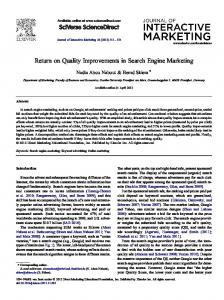
pages leading to significant improvements in the “hub” values. 10 HITS is rarely used in general web search engines since it is vulnerable to spam links (Asano, Tezuka and Nishizeki 2008); also, it is query-specific and as such has to be computed at runtime, which would in many cases prove to be too laborious. At one point, a HITS-based ranking was used by the Teoma search engine (see Davison et al. 1999). The second major link-based algorithm, PageRank (Brin and Page 1998), proved far more successful. It does not distinguish between different dimensions; instead, a single value is calculated for every page. Every link from page A to page B is considered to transfer a fraction of its own PageRank to the linked page; if a page with PageRank 10 has 5 outgoing links, it contributes 2 to the PageRank of every one of those. This process is also repeated iteratively; as it is query-independent, the PageRank values need not be calculated at runtime, which saves time. It is important to remember that these descriptions are extremely simplified versions of the actual algorithms used; that no major search engine publishes its ranking technology, though brief glimpses might be caught in patents; and that the ranking is always based on a large number of criteria. Google, for example, uses more than 200 indicators, of which the PageRank is but one (Google 2010). The leader of the Russian search engines market, Yandex, claims that the size of their ranking formula increased from 20 byte in 2006 to 120 MB in the middle of 2010 (Segalovich 2010), and to 280 MB in September 2010 (Raskovalov 2010). To put things in perspective, that is approximately 50 times the size of the complete works of William Shakespeare.11 1000000 280000
Formula size (kb)
10000
220
100 14 1
0,01
1
0,02 2006
2007
2008
2009
2010
Figure 2.1. The complication of Yandex ranking formulas (data from Raskovalov 2010; Segalovich 2010). Note that the vertical scale (formula size in kilobyte) is logarithmic.
10
To allow the results to converge and the algorithm to terminate, the hub and authority values are usually normalized after every iteration. 11 Uncompressed digital version available at Project Gutenberg (http://www.gutenberg.org/ebooks/100).
- 16 -
Many major search engines offer other types of results than the classical web page list – images, videos, news, maps and so forth. However, the present work only deals with the document lists. As far as I know, there have been no attempts to provide a single framework for evaluating all aspects of a search engine, and such an approach seems unfeasible. There are also other features I will have to ignore to present a concise case; for example, spellcheckers and query suggestions, question-answering features, relevant advertising etc. I do not attempt to discuss the usefulness of the whole output a search engine is able of; when talking of “result lists”, I will refer only to the organic document listing that is still the search engines’ stock-in-trade. This is as much depth as we need to consider search evaluation and its validity; for a real introduction to search engines, I recommend the excellent textbook “Search Engines: Information Retrieval in Practice” (Croft, Metzler and Strohman 2010).
2.2 Search Engine Usage For any evaluation of search engine performance it is crucial to understand user behavior. This is true at the experimental design stage, when it is important to formulate a study object which corresponds to something the users do out there in the real world, as well as in the evaluation process itself, when one needs to know how to interpret the gathered data. Therefore, I will present some findings that attempt to shed light on the question of actual search engine usage. This data comes mainly from two sources: log data evaluation (log data is discussed in Chapter 5) and eye-tracking studies. Most other laboratory experiment types, as well as questionnaires, interviews, and other explicit elicitations, have rarely been used in recent years. 12 Unfortunately, in the last years search engine logs have not been made available to the scientific community as often as ten years ago. The matter of privacy alone, which is at any case hotly debated by the interested public, surely is enough to make a search engine provider think twice before releasing potentially sensitive data.13 What, then, does this data show? The users’ behavior is unlike that experienced in classical information retrieval systems, where the search was mostly performed by intermediaries or other information professionals skilled at retrieval tasks and familiar with the database, query language and so forth. Web search engines aim at the average internet user, or, more precisely, at any internet user, whether new to the web or a seasoned Usenet veteran. For our purposes, a search session starts with the user submitting a query. It usually contains two to three terms (see also Figure 2.2), and has been slowly increasing during the time web search has been observed (Jansen and Spink 2006; Yandex 2008). The average query has no 12
This is probably due to multiple reasons: The availability (at least for a while) of large amounts of log data; the difficulty in inferring the behaviour of millions of users from a few test persons (who are rarely representative of the average surfer), and the realization that explicit questions may induce the test person to behave unnaturally. 13 The best-known case is probably the release by AOL for research purposes of anonymized log data from 20 million queries made by about 650.000 subscribers. Despite the anonymization, some users were identified soon (Barbaro and Zeller Jr. 2006). Its attempt at public-mindedness brought AOL not only an entry in CNN’s “101 Dumbest Moments in Business” (Horowitz et al. 2007), but also a Federal Trade Commission complaint by the Electronic Frontier Foundation (2006) and a class-action lawsuit which was settled out of court for an undisclosed amount (Berman DeValerio 2010).
- 17 -
operators; the only one used with any frequency being the phrase operator (most major engines use quotation marks for that) which occurs in under 2% of the queries, with 9% of users issuing at least one query containing operators (White and Morris 2007).14 The queries are traditionally divided into navigational (user looks for a specific web page known or supposed to exist), transactional (not surprisingly, in this case the user looks to perform a transaction like buying or downloading) and informational, which should need no further explanation (Broder 2002). While this division is by no means final, and will be modified after an encounter with the current state of affairs in Section 9.2, it is undoubtedly useful (and widely used). Broder’s estimation of query type distribution is that 20-25% are navigational, 39-48% are informational, and 30-36% are transactional. A large-scale study with automatic classifying had a much larger amount of informational queries (around 80%), while navigational and transactional queries were at about 10% each (Jansen, Booth and Spink 2007). 15 Another study with similar categories (Rose and Levinson 2004) also found informational queries to be more frequent than originally assumed by Broder (62-63%), and the other two types less frequent (navigational queries 12-15%, transactional queries 2227%).16
Figure 2.2. Query length distribution (from Yandex 2008, p. 2). Note that the data is for Russian searches.
Once the user submits his query, he is presented with the result page. Apart from advertising, “universal search” features and other elements mentioned in Section 2.1, it contains a result list with usually ten results. Each result consists of three parts: a page title taken directly from the page’s tag, a so-called “snippet” which is a query-dependant extract from the 14
For the 13 weeks during which the data was collected. A study of log data collected 7-10 years earlier had significantly higher numbers of queries using operators, though they were still under 10% (Spink and Jansen 2004). 15 While the study was published in 2007, the log data it is based is at least five years older, and partly originates in the end-90ies. 16 Note that all cited statistics are for English-speaking users. The picture may or may not be different for other languages; a study using data from 2004 showed no fundamental differences in queries originating from Greece (Efthimiadis 2008). A study of Russian log data additionally showed 4% of queries containing a full web address, which would be sufficient to reach the page via the browser’s address bar instead of the search engine. It also stated that about 15% of all queries contained some type of mistake, with about 10% being typos (Yandex 2008).
- 18 -
page, and a URL pointing to the page itself. When the result page appears, the user tends to start by scanning the first-ranked result; if this seems promising, the link is clicked and the user (at least temporarily) leaves the search engine and its hospitable result page. If the first snippet seems irrelevant, or if the user returns for more information, he proceeds to the second snippet which he processes in the same way. Generally, if the user selects a result at all, the first click falls within the first three or four results. The time before this first click is, on average, about 6.5 seconds; and in this time, the user catches at least a glimpse of about 4 results (Hotchkiss, Alston and Edwards 2005). 17 As Thomas and Hawking note, “a quick scan of part of a result set is often enough to judge its utility for the task at hand. Unlike relevance assessors, searchers very seldom read all the documents retrieved for them by a search engine” (Thomas and Hawking 2006, p. 95). There is a sharp drop in user attention after rank 6 or 7; this is caused by the fact that only these results are directly visible on the result page without scrolling.18 The remaining results up to the end of the page receive approximately equal amounts of attention (Granka, Joachims and Gay 2004; Joachims et al. 2005). If a user scrolls to the end of the result page, he has an opportunity to move to the next one which contains further results; however, this option is used very rarely – fewer than 25% of users visit more than one result page,19 the others confining themselves to the (usually ten) results on the first page (Spink and Jansen 2004).
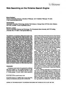
Figure 2.3. Percentage of times an abstract20 was viewed/clicked depending on the rank of the result (taken from Joachims et al. 2005, p. 156). Data is based on original and manipulated Google results, in an attempt to eliminate quality bias. Note that the study was a laboratory-based, not log-based one.
17
Turpin, Scholer et al. (2009) mention 19 seconds per snippet; however, this is to consciously judge the result and produce an explicit rating. When encountering a result list in a “natural” search process, the users tend to spend much less time deciding whether to click on a result. 18 Obviously, this might not be the case for extra high display resolutions; however, this does not invalidate the observations. 19 Given the previous numbers in this section, a quarter of all users going beyond the first result page seems like a lot. The reason probably lies in the different sources of data in the various studies; in particular, the data used by Spink and Jansen (2004) mostly stems from the 1990s. 20 “Abstract” and “snippet” have the same meaning in this case.
- 19 -
The number of pages a user actually visits is also not high. Spink and Jansen (2004) estimate them at 2 or 3 per query; and only about one in 35,000 users clicks on all ten results on the first result page (Thomas and Hawking 2006). This fact will be very important when we discuss the problems with traditional explicit measures in section 4. Most of those clicks are on results in the very highest ranks; Figure 2.3 gives an overview of fixation (that is, viewing one area of the screen for ca. 200-300 milliseconds) and click rates for top ten results. Note that the click rate falls much faster than the fixation rate. While rank 2 gets almost as much attention as rank 1, it is clicked more than three times less often.
- 20 -
3 Evaluation and What It Is About We must decide what ought to be the case. We cannot discover what ought to be the case by investigating what is the case. PAUL W. TAYLOR, “NORMATIVE DISCOURSE” The evaluation of a web search engine has the same general goal as that of any other retrieval system: to provide a measure of how good the system is at providing the user with the information he needs. This knowledge can then be used in numerous ways: to select the most suitable of available search engines, to learn about the users or the data searched upon, or – most often – to find weaknesses in the system and ways to eliminate them. However, web search engine evaluation also has the same potential pitfalls as its more general counterpart. The classical overview of an evaluation methodology was developed by TagueSutcliffe (Tague 1981; Tague-Sutcliffe 1992). The ten points made by her have been extremely influential, and we will now briefly recount them, commenting on their relevance to the present work. The first issue is “To test or not to test”, which bears more weight than it seems at a first glance. Obviously, this step includes reviewing the literature to check if the questions asked already have answers. However, before this can be done, one is forced to actually formulate the question. The task is anything but straightforward. “Is that search engine good?” is not a valid formulation; one has to be as precise as possible. If the question is “How many users with navigational queries are satisfied by their search experience?”, the whole evaluation process will be very different than if we ask “Which retrieval function is better at providing results covering multiple aspects of a legal professional’s information need?”. These questions are still not as detailed as they will need to be when the concrete evaluation methods are devised in the next steps; but they show the minimal level of precision required to even start thinking about evaluation. It is my immodest opinion that quite a few of the studies presented in this chapter would have profited from providing exact information on what it is they attempt to quantify. As it stands, neither the introduction of new nor the evaluation of existing metrics is routinely accompanied by a statement on what precisely is to be captured. There are some steps in the direction of a goal definition, but these tend to refer to behavioral observations ("in reality, the probability that a user browses to some position in the ranked list depends on many other factors other than the position alone", Chapelle et al. 2009, p. 621) or general theoretical statements ("When examining the ranked result list of a query, it is obvious that highly relevant documents are more valuable than marginally relevant", Järvelin and Kekäläinen 2002, p. 424). To be reasonably certain to find an explicit phenomenon to be measured, one needs to turn to the type of study discussed in Chapter 6, which deals precisely with the relationship of evaluation metrics and the real world. The second point mentioned by Tague-Sutcliffe concerns the decision on what kind of test is to be performed, the basic distinction being that between laboratory experiments and operational tests. In laboratory experiments, the conditions are controlled for, and the aim of
- 21 -
the experiment can be addressed more precisely. Operational tests run with real users on real systems, and thus can be said to be generally closer to “real life”. Of course, in practice the distinction is not binary but smooth, but explicit measures (Chapter 4) tend to be obtained by laboratory experiments, while implicit measures (Chapter 5) often come from operational tests. The third issue “is deciding how actually to observe or measure […] concepts – how to operationalize them” (Tague-Sutcliffe 1992, p. 469). This means deciding which variables one controls for, and which are going to be measured. The features of the database, the type of user to be modeled, the intended behavioral constraints for the assessor (e.g. “Visit at least five results”), and – directly relevant to the present work – what and how to evaluate are all questions for this step. The fourth question, what database to select, is not very relevant for us; mostly, either one of the popular web search engines is evaluated, or the researcher has a retrieval method of his own whose index is filled with web pages, of which there is no shortage. Sometimes, databases assembled by large workshops such as TREC21 or CLEF22 can be employed. More interesting is issue five, which deals with queries. One may use queries submitted by the very person who is to assess the results; in fact, this is mostly regarded as the optimal solution. However, this is not always easy to do in a laboratory experiment; also, one might want to examine a certain type of query, and so needs to be selective. As an alternative, the queries might be constructed by the researcher; or the researcher might define an information need and let the assessors pose the query themselves. As a third option, real queries might be available if the researcher has access to search engine logs (or statistics of popular queries); in this case, however, the information need can only be guessed. The question of information need versus query will be discussed in more detail in Chapter 7 which deals with the types of relevance. Step six deals with query processing; my answer to this problem is explained in Section 9.1. Step seven is about assigning treatments to experimental units; that is, balancing assessors, queries, and other experimental conditions so that the results are as reliable as possible. Step eight deals with the means and methods of collecting the data (observation, questionnaires, and so forth); steps nine and ten are about the analysis and presentation of the results. These are interesting problems, but I will not examine them in much detail in the theoretical part, while trying to pay attention to them in the actual evaluations we undertake. Tague-Sutcliffe’s paradigm was conceived for classical information retrieval systems. I have already hinted at some of the differences search engine evaluation brings with it, and more are to come when evaluation measures will be discussed. To get a better idea of the entities search engine evaluation actually deals with, I feel this is a good time to introduce our protagonists.
21 22
Text REtrieval Conference, http://trec.nist.gov Cross-Language Evaluation Forum, http://www.clef-campaign.org
- 22 -
4 Explicit Metrics Don’t pay any attention to what they write about you. Just measure it in inches. ANDY WARHOL The evaluation methods that are most popular and easiest to conceptualize tend to be explicit, or judgment-based. This is to be expected; when faced with the task of determining which option is more relevant for the user, the obvious solution is to ask him. The approach brings with it some clear advantages. By selecting appropriate test persons, one can ensure that the information obtained reflects the preferences of the target group. One can also focus on certain aspects of the retrieval system or search process, and – by carefully adjusting the experimental setting – limit the significance of the answers to the questions at hand. The main alternative will be discussed in Chapter 5 which deals with implicit metrics. Section Group Metrics 4.1 Recall/Precision and their Precision direct descendants Recall Recall-precision Graph F-Measure F1-Measure Mean Average Precision (MAP) 4.2 Other system-based Reciprocal Rank (RR) metrics Mean Reciprocal Rank (MRR) Quality of result ranking (QRR) Bpref Sliding Ratio (SR) Cumulative Gain (CG) Discounted Cumulative Gain /DCG) Normalized Discounted Cumulative Gain (NDCG) Average Distance Measure (ADM) 4.3 User-based metrics Expected Search Length (ESL) Expected Search Time (EST) Maximal Marginal Relevance (MMR) α–Normalized Discounted Cumulative Gain (α-NDCG) Expected Reciprocal Rank (ERR) 4.4 General problems of explicit metrics Table 4.1. Overview of evaluation metrics described in this section.
We will first recapitulate the well-known concept of recall and precision and consider the measures derived from it (Section 4.1). Then we will describe some further measures which focus on the system being evaluated (Section 4.2), before turning to more user-based measures (Section 4.3). Finally, we will discuss problems common to all explicit measures and ways suggested to overcome them (Section 4.4). An overview of all described metrics can be found in Table 4.1.
- 23 -
4.1 Recall, Precision and Their Direct Descendants Precision, probably the earliest of formally stated IR evaluation measures, has been proposed in 1966 as part of the Cranfield Project (Cleverdon and Keen 1968). The basic idea is very simple: the precision of a retrieval system for a certain query is the proportion of results that are relevant. A second proposed and widely used metric was recall, defined as the proportion of relevant results that have been retrieved.
Formula 4.1. Precision
Formula 4.2. Recall
The recall and precision measures are generally inversely proportional: if a retrieval system returns more results, the recall can only increase (as the number of relevant results in the database does not change), but precision is likely to fall. This is often captured in the so-called recall-precision-graphs (see Figure 4.1).
Figure 4.1. Example of a recall-precision graph showing the performances of different retrieval systems (from Voorhees and Harman 2000, p. 14). The graph visualizes the typical trade-off between recall and precision faced by any IR system. When the recall reaches 1, that is, when every document is retrieved, the precision is at its lowest; when precision is highest, it is recall that plummets. Every system has to find a balance reflecting the expected needs of its users.
- 24 -
To combine these two aspects of retrieval, the F-Measure was introduced (Van Rijsbergen 1979). It is an indicator for both recall and precision, with the relative importance set by the weighting constant β. In the special but frequent case of recall and precision being equally important (β=1) the formula reduces to the so-called F1 score. In this case (or with any β close to 1), either low precision or low recall leads to a low overall rating. With a β closer to 0, precision has a larger influence on the F-Measure, while a β higher than 1 means recall is more important.
Formula 4.3. F-Measure for precision P and recall R. β is a constant which can be used to influence the relative importance of recall and precision.
Formula 4.4. F1-Measure for precision P and recall R; it corresponds to the F-Measure with β set to 1.
As has often been noted, “since the 1950’s the adequacy of traditional measures, precision and recall, has been a topic of heated debates […], and at the same time of very little experimentation” (Su 2003, p. 1175). It was argued that these measures might work well for a relatively small-scale IR system used by information professionals or experienced researchers. But for other uses, their practical and theoretical limitations become apparent. It stands to reason that for large databases with millions of documents recall cannot be easily determined, as it depends on knowing the precise number of relevant documents in the database. 23 Furthermore, as the quantity of returned results increases, it becomes difficult to rate the relevance of each one manually. Especially in web search engines, where there may be millions of relevant results,24 it is impossible to evaluate each one. The solution comes from studies showing that users look only at a small number of results, with most users restricting themselves to just the first result page (Jansen and Spink 2006). Thus, evaluating all returned results becomes at least unnecessary, and, if one focuses on the user experience, may even be counterproductive. One further problem remains, however. Precision treats all returned results equally; but as the user’s attention decreases, pages in the lower parts of the result list become less important, and may not be considered at all (Jansen et al. 1998). Therefore, most modern metrics, precision-based metrics among them, include some kind of damping constant that discounts the value of later results. One of the most popular measures is the Mean Average Precision (MAP). As its name suggests, it averages mean precisions 25 of multiple queries. In words,
23
This problem was at least partially alleviated by the employment of methods such as Relative Recall (Clarke and Willett 1999). As recall is not a primary issue of the present work, it will not be discussed further. 24 At least, those are the numbers estimated and displayed by major search engines. In practice, only a subset of those is actually returned in the result list, mostly under a thousand pages. This aggravates the problem, as the results are usually still too many to rate, but now precision cannot be calculated even in theory, lacking the complete list of returned results. 25 “It means average precisions” would have the words in a more appropriate order, but seems a bit ambiguous.
- 25 -
MAP considers the precision at every relevant result in the list; then, the precision is averaged by dividing the sum of discounted precisions by the total number of relevant results.26 AP
1
∑
1 | |
| |
∑rk 1 rel d r
∑
i
Formula 4.5. MAP formula with queries Q and documents D. dr is a document at rank r. rel is a relevance function assigning 1 to relevant and 0 to non-relevant results.
An example may be appropriate do demonstrate the calculation of MAP. Given the imaginary relevance judgments in Table 4.2, and supposing no further relevant documents are known to exist, the explicit calculation is given in Figure 4.2. For comparison: The precision for each of the queries is 0.6. Query 1 Query 2
Result 1 1 0
Result 2 1 0
Result 3 0 1
Result 4 1 1
Result 5 0 1
Table 4.2. Imaginary binary relevance for results of two queries.
( (
))
( (
))
Figure 4.2. MAP calculation for values in Table 4.2.
MAP is one of the most-used metrics and is employed in single studies as well as in large efforts such as TREC (Clarke, Craswell and Soboroff 2009). However, it is also not without its problems. In particular, some studies have detected a lack of correlation between MAP and actual user performance (Hersh et al. 2000; Turpin and Hersh 2001). These studies are based upon data collected in the TREC Interactive Track (see Hersh and Over 2000), which is assessed by asking users to find one or more answers to predefined questions in a given time. The number of answers or instances they collect can be used as a standard against which to rate other, more system-centered metrics. The results show that an increase in MAP need not correspond to a significant, or indeed any, increase in user performance. Turpin and Hersh have also looked in more detail at the possible reasons for this discrepancy; their finding is that, while users encounter more non-relevant results, the number of relevant results stays constant. They conclude that the users are not hindered much by a low Mean Average Precision. The two studies had a relatively small number of queries; furthermore, it could be argued that the setting of a fixed search time significantly distorts the users’ real-life behavior and cannot be transferred to other fields such as classical web search. For example, the assessors were not supposed to abandon the search ahead of time if they grew frustrated with the high number of non-relevant results. However, the user model implied by this limit is conceptually not less
26
Note that this is not the number of returned relevant results but the number of all relevant results in the database, or at least the number of relevant results known to exist.
- 26 -
realistic than MAP which does not assume a user model at all; at the very least, the studies have to be taken seriously and their claims kept in mind. The findings were also strengthened in a study concerning itself with more simple – and presumably more common – tasks (Turpin and Scholer 2006). A first task was precisionbased; it required the users to find a single relevant result for a pre-defined TREC query. The ranking algorithms were selected as to reflect a range of MAP values from 55% to 95%. For every algorithm, the average time elapsed before answer is found and the average percentage of sessions where no relevant document was found were calculated. Neither had any significant correlation to MAP, or to precision at ranks 2, 3, 4 and 10. The only (weak) correlation was observed for precision at rank 1; however, the authors note that this might be an effect of the study design. A second task was recall-based; the users were asked to identify as many relevant documents as possible in a fixed time period. Again, the different ranking algorithms were employed. The only statistically significant differences were observed between the pairs 55% vs. 75% and 65% vs. 75%. However, since the absolute improvement was very low (extra 0.3 documents per session), and the user performance fell again in the conditions featuring MAP values of 85% and 95%, the correlation does not seem impressive. Though some objections against the methodology of the study could be made – the authors mention the different user groups for the TREC-rated documents and the student-performed retrieval task – it clearly adds much doubt to MAPs appropriateness as a measure of probable user performance. Slightly better correlation between precision and user satisfaction was shown by Kelly, Fu and Shah (2007). They performed a test on four topics from TREC newspaper data. Each subject was given a topic statement and was instructed to construct a query; however, the user was presented with a result list that was fixed in advance and did not depend on the actual query but solely on the topic. There were four result lists; in one condition, they significantly differed in precision, while being similar in MAP (more scattered relevant results versus few relevant results at top ranks), while in another, the precision was equal, but the ranking different (e.g. ranks 1-5 relevant and 6-10 irrelevant, or vice versa). The users were asked to rate single documents as well as the overall performance of every “search engine”. The results showed that, with higher MAP as constructed from users’ document ratings, the rating of the result list also tend to grow. However, the correlation was only significant for less than half of all users; in fact, users with average ratings for documents as well as result lists were the only group showing this significance. Furthermore, the study has some serious methodological issues. First, there were only four topics, a very small sample. Second, the result lists were not query-specific but topic-specific; this must have lead to different search experiences and different relevance ratings among users. Finally, the result lists were constructed using expected precision values derived from TREC ratings; however, no statistics on their correlation with user assessments of result set quality are provided.
4.2 Other System-based Metrics A simple measure intended for a specific task is the Mean Reciprocal Rank (MRR). Reciprocal Rank (RR) is defined as zero if no relevant results are returned, or else one
- 27 -
through the rank of the first encountered relevant result (Formula 4.6). For MRR, the mean of RR values for single queries is taken (Voorhees 1999). MRR assumes that the user is only interested in one relevant result, and anything following that result is irrelevant to his search experience (see Formula 4.7). This seems to be an intuitive assumption for some types of queries, particularly navigational ones.
{
Formula 4.6. Reciprocal Rank (RR), with r the first rank where a relevant result is found.
| |
∑
Formula 4.7. Mean Reciprocal Rank (MRR), Q being the set of queries and RRq the Reciprocal Rank measured for query q.
A metric proposed explicitly for web search evaluation is the Quality of result ranking (QRR; Vaughan 2004). It is quite unusual among explicit measures in the way it constructs its rating. First, human judgments are obtained for the search results in the usual way. Preferably, the results will be pooled from several search engines’ lists for the same query. In the next step, however, those are used to construct an alternative result list, one that is sorted by userassigned relevance. This is compared to the original result lists provided by the search engines, and a correlation coefficient is calculated. Vaughan provides an evaluation of her metric. Vaughan applies QRR to three search engines and finds that the results are significantly different. From that, she concludes that it is “able to distinguish search engine performance” (Vaughan 2004, p. 689). This, however, seems to be an example of a vicious circle; the metric is valid because it “recognizes” a difference, which is assumed on the basis of the metric. QRR itself has not been widely used for evaluations; however, it deserves attention for its attempt to detect correlations. We will encounter more correlation-based measures when dealing with implicit measurements; in particular, the notion of Normalized Discounted Cumulated Gain later in this section follows a similar logic. A measure which has enjoyed some exposure, for example at a few of the TREC tracks, is bpref,27 so called “because it uses binary relevance judgments to define the preference relation (any relevant document is preferred over any nonrelevant document for a given topic)” (Buckley and Voorhees 2004, p. 26). This is unusual among explicit metrics, as it does not attempt to assign an absolute rating to results, but merely to find pairs where one document should be preferable to another. The metric, given in Formula 4.8, calculates the number of non-relevant documents n ranked higher than a relevant document r, and averages the number over the first R relevant results.28 Bpref was shown to correlate well (with Kendall τ>90%) 27
The authors write “bpref” with a lower-case “b” except in the beginning of a sentence, where it is capitalized. I do not see any reason not to follow their approach – after all, they should know best. 28 To ensure that the values fall into the [1..0] interval, n is also restricted to the first R occurrences.
- 28 -
with MAP, while being more stable when fewer judgments are available. Also, increases in bpref were correlated to lower times for task completion and higher instance recall in a passage retrieval task, although the connections are not linear, and may not apply to other retrieval tasks (Allan, Carterette and Lewis 2005). ∑
|
|
Formula 4.8. Bpref (Buckley and Voorhees 2004). Its distinguishing characteristic is the comparison of results within a result list. For each relevant result r (up to a predetermined number of relevant results R), the number of nonrelevant results n above it in the list is calculated, and the results average over the different r’s. Thus, every nonrelevant result ranked higher than a relevant one causes bpref to decrease from its maximum value of 1.
There has also been the rpref metric, introduced mainly to allow for graded instead of binary relevance (De Beer and Moens 2006). However, neither bpref nor its modification will play a significant role in the current evaluation. The reason is that these metrics are explicitly designed for situations where relevance judgments are incomplete. In the study presented in Part II, this problem does not occur, for reasons that will be discussed in the methodological Section 9.1. Additionally, it has been suggested that even in the very circumstances it has been conceived for, bpref performs worse than traditional metrics. When non-judged results are simply disregarded, metrics like Average Precision or NDCG show more robustness and discriminatory power than bpref or rpref (Sakai 2007a). An early measure comparing a system’s actual result list to an idealized output is the Sliding Ratio (Pollock 1968). It is calculated as the ratio of the actual retrieval system’s score to an ideal ranking of the same documents for every rank up to a certain threshold; hence the name. In Formula 4.9, c is the cut-off value (the number of results considered), rel(dr) the relevance (or weight) of the document at rank r, and rel(drideal) the relevance of the r-th result in an ideally ranked result list. The simple sample shown in Table 4.3 illustrates that since only the retrieved documents are considered for the construction of the ideal ranking, the SR at rank n is always 1. ∑ ∑ Formula 4.9. Sliding Ratio (Korfhage 1997)
Rank 1 2 3 4 5
Relevance 1 2 3 4 5
Ideal relevance at rank 5 4 3 2 1
Sliding Ratio 0.2 0.33 0.5 0.71 1
Table 4.3. Example of Sliding Ratio calculation
A measure which has enjoyed wide popularity since its introduction is Discounted Cumulated Gain or DCG for short (Järvelin and Kekäläinen 2000). The more basic measure upon which it is constructed is the Cumulated Gain, which is a simple sum of the relevance judgments of
- 29 -
all results up to a certain rank. DCG enhances this rather simple method by introducing “[a] discounting function [...] that progressively reduces the document score as its rank increases but not too steeply (e.g., as division by rank) to allow for user persistence in examining further documents” (Järvelin and Kekäläinen 2002, p. 425). In practice, the authors suggest a logarithmic function, which can be adjusted (by selecting its base) to provide a more or less strong discount, depending on the expectations of users’ persistence. { Formula 4.10. DCG with logarithm base b (based on Järvelin and Kekäläinen 2002). CGr is the Cumulated Gain at rank r, and rel(r) a a relevance function assigning 1 to relevant and 0 to non-relevant results.
Query 1 CQ DCQ log2 Query 2 CQ DCQ log2
Result 1 1 1 1 0 0 0
Result 2 1 2 2 1 1 1
Result 3 0 2 2 1 2 1,63
Result 4 1 3 2,5 1 3 2,13
Result 5 0 3 2,5 0 3 2,13
Table 4.4. CG and DCG calculation for values from Table 4.2.
One weak point of DCG is the missing comparability to other metrics as well as between different DCG-evaluated queries. Should one query be “easy” and have more possible relevant hits than another, its DCG would be expected to be higher; the difference, however, would not signify any difference in the general retrieval performance. A measure which indicates retrieval quality independent from the quality of available results (that is, from the “difficulty” of the search task) would be more helpful. To remedy the situation, Normalized DCG (NDCG) can be employed. NDCG works by pooling the results from multiple search engines’ lists and sorting them by relevance. This provides an “ideal result list” under the assumption that all the most relevant results have been retrieved by at least one of the search engines. The DCG values of the single search engines can then be divided by the ideal DCG to put them into the [0..1] interval, with 0 meaning no relevant results and 1 the ideal result list.29 Note, however, that NDCG is quite similar to a version of Sliding Ratio with added discount for results at later ranks. The authors evaluated the different CG measures (Järvelin and Kekäläinen 2000; Järvelin and Kekäläinen 2002). However, this was not done by comparing the new measure with a standard, or with established measures; instead, it was used to evaluate different IR systems, where one was hypothesized to outperform the others. The CG measures indeed showed a significant difference between the systems, and were considered to have been validated. I think this methodology is not quite satisfactory. It seems that evaluating the hypothesis with 29
Obviously, if the ideal DCG is zero, the calculation is not possible. However, this is not a large problem, since this value would mean no relevant pages are known, and such a query would probably best be excluded from the evaluation altogether. Alternatively, if relevant documents are supposed to exist, they can be explicitly added into the ideal ranking, either on a per-query basis or as a default baseline across all queries.
- 30 -
the new measure while at the same time evaluating the new measure against the hypothesis may produce a positive correlation without necessarily signifying a meaningful connection to any outside entity. However, a more stringent evaluation of DCG was performed by AlMaskari, Sanderson and Clough (2007). In the study, Precision, CG, DCG and NDCG were compared to three explicit measures of user satisfaction with the search session called “accuracy”, “coverage” and “ranking”. The results were mixed. From the overall 12 relations between metric and user satisfaction, only two showed a significant correlation, namely, Precision and CG with the ranking of results. Unfortunately, the authors provide no details as to what the assessors were instructed to rate by their satisfaction measures; it seems possible that, say, a user’s perception of accuracy may well be influenced by the result ranking. Still, the study is the only one I know of that directly compares the CG family to user satisfaction, and its results are only partly satisfactory. These results notwithstanding, (N)DCG is conceptually sound, and provides more flexibility than MAP. Since its introduction in 2000, it has become one of the most popular search engine evaluation measures; and we definitely do not mean to suggest throwing it overboard as soon as some initial doubt is cast on its correlation to real-world results. ∑
|
| | |
Formula 4.11. ADM for retrieved documents D, System Relevance Score SRS and User Relevance Score URS
A measure which is rarely used for actual evaluation but provides some interesting aspects for the current study is the Average Distance Measure (ADM). It has been introduced explicitly to replace existing measures which were considered to rely too heavily on binary distinctions. The distinction between relevant and non-relevant documents is opposed to documents lying along a scaled or continuous relevance axis, and that between retrieved and non-retrieved documents is to be smoothed by considering the rank of the retrieved result (Mizzaro 2001; Della Mea et al. 2006). The ADM measure is, in short, the average difference between a system’s and a user’s relevance scores for the documents returned for a query. The interesting characteristic of ADM is that, while it attempts to distinguish itself from precision in some aspects, it is similar in that it is an extremely system-based measure, focusing on single system ratings rather than on user experience. To provide a simple example, a retrieval system providing a bad result list but recognizing it as such can get an ideal ADM (since its evaluation of the results’ quality is perfect); one that provides ideal results but regards them as mediocre them performs worse (since it underestimates the result quality). 30 Evaluation results calculated using ADM have been compared to those produced by Average Precision, and found not to correlate with it (Della Mea, Di Gaspero and Mizzaro 2004); however, this merely means that the two measures do not evaluate the same aspects of search engines. Both still may be good at specified but distinctly different tasks.
30
Also, AD
obviously depends on a system’s relevance scores for documents, which are not readily available.
- 31 -
4.3 User-based Metrics Another class of metrics goes beyond relevance by employing models of user behavior. The distinction is somewhat vague since any discounted metric such as MAP or DCG already makes some assumption about the behavior, viz. the user being more satisfied with relevant results in earlier than in later ranks. DCG even provides a method for adjusting for user persistence by modifying the logarithm base of its formula. Still, it can be argued that the measures to be presented in this section differ significantly by explicitly stating a user model and constructing a metric to reflect it. The rationale for turning away from purely systembased measures was nicely formulated by Carbonell and Goldstein: Conventional IR systems rank and assimilate documents based on maximizing relevance to the user query. In cases where relevant documents are few, or cases where very-high recall is necessary, pure relevance ranking is very appropriate. But in cases where there is a vast sea of potentially relevant documents, highly redundant with each other or (in the extreme) containing partially or fully duplicative information we must utilize means beyond pure relevance for document ranking.31 (Carbonell and Goldstein 1998, p. 335)
An early metric focusing on the user’s information need is Expected Search Length (ESL). It is defined as the number of non-relevant documents in a weakly ordered document list a user has to examine before finding n relevant ones (Cooper 1968). It may be viewed as a more general version of Mean Reciprocal Rank (MRR), which is analogous (or, rather, inversely proportional) to ESL with n=1. It should also be noted that the number of retrieved relevant documents is not the only variable; the definition of relevance can also be set so as to model a user’s information need. One problem with ESL is the underlying assumption that user satisfaction is primarily influenced by non-relevant results. This is not self-evident; indeed, some studies suggest that at least in some circumstances, the number of non-relevant results plays hardly any role (Turpin and Hersh 2001). For this and other reasons, ESL was expanded by Dunlop (1997) to an “Expected Search Time” (EST) measure. By estimating the time needed to interact with the search engine (to read an abstract, to read a document and so forth), he comprised a metric for the probable duration of a user’s search session before he finds the n relevant results he needs. However, further limitations of EST as well as ESL remain; the number of desired relevant documents may vary heavily depending on the information need as well as on the individual user. Also, a user himself probably does not know how many documents he will require; he may prefer all the information to be in a single document, but if it is scattered, he might really want all five or ten relevant documents. A measure concerned with the diversity of the result list is the Maximal Marginal Relevance, or MMR (Carbonell and Goldstein 1998). It assumes that the user wishes to encounter documents which are as similar as possible to the query, but as dissimilar as possible between 31
Here, “relevance” is taken to mean the objective relevance of a single document to a query (topicality). Relevance is discussed in more detail in Chapter 7.
- 32 -
each other so as to avoid duplicate information. In short, MMR finds, for any rank, the document for which the difference between query similarity (topicality) and similarity to already retrieved documents (repetition of information) is maximal. A parameter can be used to assign relative importance to the two concepts; if it is set to 1, the novelty factor disappears, and MMR is reduced to a standard topicality measure. If it is 0, the topicality is disregarded, and novelty remains the only factor. The concept of marginal relevance is especially interesting since it neatly encompasses the economic notion that only new information is useful (Varian 1999). MMR was conceived as a ranking function, but, it can easily be adapted for evaluation. However, since it requires a sophisticated similarity measurement, it will not be employed in the study presented in Part II (and I will spare you a complicated formula). MMR’s approach is to start from first principles; an alternative is to take existing measures and expand them by adding a novel user model. One such measure is α-NDCG, which adds to the (normalized) DCG score the concepts of users’ information needs as well as novelty and relevance rating details (Clarke et al. 2008). It employs the concept of an “information nugget” which has gained acceptance in several IR subfields (Dang, Lin and Kelly 2006). In the context of α-NDCG, “information nugget” denotes any property of the document which might be relevant to the user. Thus, a document can have no, one or multiple useful information nuggets. The metric then proceeds with some quite complex calculations, determining the probability that a user will find nuggets in the current document as well as the probability for each nugget that it has already been encountered during the search session. These two probabilities then determine the gain at the current rank, which is handled similarly to the gains in usual NDCG. Once again, it is too complex for the present evaluation, and is mentioned mainly because it shows the sophistication of user models that can be employed by current metrics. An example of a novel evaluation metric with a different agenda is the Expected Reciprocal Rank (ERR). Whereas α-NDCG pays particular attention to the diversity and novelty of the information nuggets, ERR focuses on the documents’ cumulated probability of being useful enough to satisfy the user’s information need. In practice, this means examining whether the documents earlier in the result list have been useful; if so, the value of a new document is discounted accordingly (Chapelle et al. 2009). ∑ ∏ Formula 4.12. ERR formula. For each rank r, the probabilities of a relevant result at each earlier rank i are multiplied; the inverse probability is used as a damping factor for the gain at the current rank.
The calculation of ERR shown in Formula 4.12 shows a structure similar to those of traditional measures like MAP, with a summation over document ratings g (here as
to
indicate a slight probability that even the best-rated result might not satisfy the user
- 33 -
completely) and a rank-based discounting function 1/r. 32 The novel part is that every addend is also discounted by a factor indicating how likely it is that the user has already found enough information not to be interested in the current result; the factor is the product of previous results’ weights, each subtracted from 1 to provide higher discount for better previous results.
4.4 General Problems of Explicit Metrics There are some problems common to all the explicit ratings described above. This section provides an overview and indicates where solutions may be found. Firstly, user judgments tend to be hard to obtain, as they require considerable resources. For the quantities of judgments needed for study results to be stable and significant, these resources may surpass the capabilities of single research groups. This is less of a problem for businesses and large collective coordinated such as TREC. However, commercial research does not always find its way into public availability; and the amount of work put into every large-scale evaluation such as TREC means there is likely to be a limited number of methods for which user judgments will be provided, and those methods are likely to be wellestablished and already tested. The second issue is the one partially addressed by user-based metrics. The explicit relevance judgments are almost always collected for individual results, and then combined in a certain way to deduce a measure of user satisfaction. The raters do answer the questions asked of them; but it is important to know whether those questions really relate to the point at stake. It is the downside of the precision advantage offered by explicit user judgments: The results are focused, but the focus may be too narrow. It has been argued, for example, that the concentration on individual results is counterproductive and should be replaced or at least supplanted by methods taking into account the user’s interaction with the result list as a whole (e.g. Spink 2002; for an overview, see Mandl 2008). Indeed, there are studies that suggest that discounting for rank and even for previously encountered relevant documents does not always alleviate the problems. One such study tested four models of user behavior as related to position bias of search engines (Craswell et al. 2008). Among them are a baseline model (no positional bias at all; clicks are based only on the snippet quality), an examination model (the probability of a click is based on position-based chance of snippet examination and snippet quality), and a cascade model (clicks are based on the attractiveness of previous snippets and the snippet of the examined document). The models were trained on data acquired from “a major search engine” (the study has been performed at Microsoft), where the results were manipulated as follows: for a subset of users, adjacent results from the first result page were swapped (e.g., the first result with the second or the 9th with the 10th). The difference in click occurrence was measured, and used to train the individual models. The predictions of these models were then compared to the actual click data.
32
As the authors note, “there is nothing particular about that choice” (Chapelle et al. 2009, p. 624); another function can be easily employed if it promises closer correspondence with the assumed user model.
- 34 -
Figure 4.3. Entropy evaluation for different position bias models (Craswell et al. 2008). A value of 0 means a perfect method; 1 is set to the baseline level.
The results, based on over 100,000 data sets, are very interesting. In short, the cascade model performs better than all the others, while the examination model produces results barely above the baseline (see Figure 4.3). This is remarkable, especially given that the cascade model used here was deliberately kept very simplistic and used some crude assumptions (such as there always being one and only one click per query). The obvious conclusion would be that a measure comprised of ratings for single results does not lead to a coherent representation of a user’s probable behavior, even if position bias is taken into account. However, the results also show that the strength of the cascade model lies in predicting the user behavior for the very first ranks. At the first rank,33 its performance is superb; at the second, good; at the third, unremarkable. From the fourth result on, the cascade model actually performs worse than the baseline model, which assumes no positional bias at all. The authors “take this to mean that there is a small amount of presentation bias at lower ranks, and a large amount of variability because clicks are rare” (Craswell et al. 2008, p. 93). This is not the only possible interpretation. Another is that the difference is not primarily one of rank, but of query type. In this reading, the model performs very well on navigational queries, which indeed contain only one result that the user is interested in, as assumed by the model. Furthermore, these results are usually near the top of the result list, in the positions where the cascade model is strongest. Broad informational queries, in contrast, tend to require multiple documents to satisfy the information need. Also, the results for non-navigational queries are considered to be more difficult to rank (Dupret and Liao 2010), so that the ranking list might be worse to begin with, allowing a relatively good performance of the baseline model. If this interpretation is correct, different metrics would be required in order to adequately assess different query types. 33
That is, when the first result is switched with the second; the rank indicates the first of two consecutive swapped results.
- 35 -
Whatever the precise reasons for the cascade model’s performance, the overall results of the study seem to indicate that the methods for using explicit relevance ratings to construct result list evaluations, as they are mostly applied today, do not correspond well with real-life user behavior. There have been further studies indicating the need for more holistic ratings. Ali, Chang et al. (2005) have shown that the correlation between result-based DCG scores and result list scores (on a tertiary scale) is 0.54 for image and 0.29 for news search. While the fields were more specific than general web search, the numbers clearly do not indicate a reliable link between the scores. Instead, the low correlation indicates that a result list might be larger or smaller than the sum of its parts; that is, good individual results might combine into a bad result list, and a result list judged to be of high quality might consist of results which are, on average, considered individually to be low-grade. A further study examined the correlation between average precision and user success (AlMaskari et al. 2008). For a number of TREC topics, test runs were performed on three search engines to determine their average precision. Then, users were presented with the best or the worst of the search engines for each topic, and were instructed to find as many relevant documents as possible in 7 minutes. The results showed a strong correlation between average precision and user success metrics (such as the number of retrieved documents) as well as user satisfaction. However, a number of conceptual issues might be raised. The correlation values are significant; but the increase in average precision that they correlate with is fourfold, which is quite an extraordinary difference. Compared with this distinction, the increase in user success and especially user satisfaction is quite low. When the (absolute or relative) difference between the systems’ average precision was reduced, the significance of correlations promptly dropped and all but disappeared when the increase in average precision was at 30%. The topics were taken from TREC, and the “title” and “description” fields were used as queries for precision calculation; however, the users searched with queries of their own, so that the correlation was actually between the precision of one query and the output and user satisfaction of another query. The average precision was very low (0.09 to 0.16 for the three search engines tested); this might be a consequence of measuring it for all results, without a cut-off value.34 This makes the “good” systems not very good, and the average precision not very realistic with regard to actual user behavior. Furthermore, the interface used by the study does not have much resemblance to the interface of most search engines, providing less transferrable results, and also aggravating possible effects an artificial setting has on user behavior. Perhaps most significantly, the task itself, with its fixed time frame and requirement of relevant document recall independent of the actual novelty or usefulness of documents, seems to be more of a task one would like to measure with average precision than a typical information need of a web searcher. This would also explain why precision@200 was found to correlate better with user’s effectiveness than average precision; since the users were 34
The authors, at least, do not mention a cut-off value, so we assume the average precision was that of all returned results.
- 36 -
instructed to gather as many relevant documents as possible, and given a fixed (and not very small) amount of time, rank effects probably did not play a major role in this evaluation. This long list of possible error sources stresses the necessity of careful consideration of study setups. One other possible explanation of the different correlations is provided by Smith and Kantor (2008). They studied the influence of degraded search quality on user performance. The degrading was achieved by returning standard Google results for the control group, and Google results starting at rank 300 for the treatment group.35 The lower quality was confirmed by significantly lower precision and (relative) recall numbers. The users were asked to find as many good sources for the topics as they could. There was no significant difference between the numbers of good results marked by the users, neither in absolute nor in relative terms. The authors conjecture that the users adapt their behavior to the change in result quality; an assumption supported by collected implicit metrics (for example, users working on “bad” result lists tended to pose significantly more queries per topic). Regrettably, the study provides no user satisfaction measures. Those would be quite interesting, as the results seem to suggest that if the correlation between precision and user performance is high, and correlation between precision and user satisfaction is low, as suggested by other studies (e.g. Turpin and Scholer 2006), there might not be any direct relationship between user performance and user satisfaction. Instead, the difference between performance and satisfaction may be caused by user effort (in this case, issuing more queries, and perhaps spending more time considering non-relevant abstracts and documents in search for relevant ones). One more study which examined the relationship between explicit relevance ratings and user satisfaction has been conducted at Google (Huffman and Hochster 2007). It used 200 random queries from those posed to the search engine, asking raters to infer probable information needs and to provide further information on the query (e.g. navigational versus informational versus transactional). Then, one set of raters was presented with the information need and the Google result list for the query, and asked to perform a normal search. After the user indicated he was done, an explicit satisfaction rating was solicited. A second group of raters was asked to give relevance ratings for the first three documents of each result list. A simple average precision at rank 3 had a very strong Pearson correlation of 0.73 with user satisfaction, which is quite a high number for so simple a metric. A higher correlation was observed for highly relevant results; this means that with really good results in the top 3 ranks, the user will not be unsatisfied. This is not really surprising; however, we have seen that studies do not always support intuitions, so the results are valuable. By manipulating the metric (in ways not precisely specified), the authors managed to increase correlation to over 0.82. The important adjustments were for navigational queries (where the relevance of the first result was given a more important role, and further results were discounted stronger), and for the number of events (such as clicks) during the session.
35
There was also an intermediate condition providing, for different topics, results starting at different ranks, from 1 to 300; the findings for this treatment were mixed, and will not be detailed here.
- 37 -
There might be multiple reasons for the fact that the Huffman and Hochster study (2007) provides a strong correlation between precision and user satisfaction while most other studies do not. First, the queries used and the tasks posed were those of real search engine users, something that other studies rarely featured. Second, the relevance considered was only that of the first three results. Studies have shown that on the web, and especially at Google, the first three or four results are the most often viewed and consequently the most important ones (Hotchkiss, Alston and Edwards 2005). This might mean that the relevance ratings of lowerranked results do not play an important role for many queries, and as such only complicate the overall picture. It would have been interesting to see how the correlation changed for average precision at, say, 10 results; that is something that will be addressed in the evaluation performed in Part II.
Figure 4.4. Session satisfaction vs. first-query relevance (modified from Huffman and Hochster 2007, p. 568). Crosses mark misspellings. The red circles indicate data points which do not have any further points with higher relevance and lower satisfaction; for all other points, a positive change in relevance might, even within the data set of that study, come with a decline in satisfaction.
Perhaps more importantly, one has to keep in mind that correlation is not everything. The models described by Huffman and Hochster may help to provide an answer to the question “Will the user be satisfied with his search session, given certain relevance rankings?”. But they are probably significantly worse at another task: judging whether a certain change in indexing or ranking procedures improves performance. The authors write: “Relevance metrics are useful in part because they enable repeated measurement. Once results for an appropriate sample of queries are graded, relevance metrics can be easily computed for multiple ranking algorithms” (Huffman and Hochster 2007, p. 571). However, if we look at the relevancesatisfaction-plot (Figure 4.4), we see that there are at most 14 data points (circled in red) which do not have further results right and down from them; that is, where increased relevance might not correspond to decreased satisfaction. If we discard misspellings, this means that only less than 10% of all data points in this sample cannot be actually worsened by - 38 -
a result set with a higher relevance score. Without access to the raw data of the study, it is difficult to tell how well these models predict exact satisfaction values given a relevance rating and – related to that and important in a practical sense – the direction of change in satisfaction given a certain (usually relatively small) change in the relevance ranking. These questions will also be followed up in Part II, where they will be answered based on new data. Similar results were also produced in a Yahoo study aimed mainly at goal success determination from user behavior (Hassan, Jones and Klinkner 2010). The average precision of the top 3 results had an 80% accuracy in predicting goal success, while DCG offered 79% (here, the considered rank was not disclosed). A Markov Model trained on query reformulation and click data provided 85% accuracy. However, one has to note that this study differed from most others in that it considered success as a function of sessions instead of the more usual queries. Also, success was estimated not by the originators of the information need but by company-internal editors.
- 39 -
5 Implicit Metrics The character of the logger’s admiration is betrayed by his very mode of expressing it... He admires the log. HENRY DAVID THOREAU, “THE ALLEGASH AND EAST BRANCH” The measures described in this section are not acquired by asking the user, as was the case with explicit ones. Instead, they are calculated using search engine logs. Logs are documents automatically created by the search engine’s servers which record user actions. Typical contents of a log are a user ID, a session ID, the query, the result list and a timestamp. The user ID is an identifier which allows tracking the user’s progress through different sessions. In the log’s original state, this is normally the user’s IP address. The session ID is a limited form of a user ID; its precise form depends on the definition of “session” used. This may range from a single query to a timeframe of many hours, during which the user submits multiple queries. The query is just the query in the form submitted by the user; it is paired with the result list. The result lists contains not just the URLs of the results offered to the user; it also shows which of the results have been clicked on. Finally, the timestamp provides information on the exact moment of the query, and – if available – the time of each individual click (Croft, Metzler and Strohman 2010). It is also important to note what the logs of a search engine do not usually contain, not least because much of the research on implicit metrics has used features not readily available. Some of these features are viewing time for a document (“How long did the user stay on a web page he found through his search?”), the amount of scrolling (“How far down the document did the user go?”), or the bookmarking or printing of a document (Kelly and Teevan 2003). Also, the logs do not provide any information as to the users’ information needs, a topic that will be discussed in Chapter 7. It is especially the click data from the result list that provides the basis for analysis. Different explanations have been proposed as to how exactly the click data corresponds to user preferences, and some of those explanations will be presented in this section. As clicks and other log data reflect user behavior, a user model is indispensable in analyzing the data; therefore, those measures lean towards the user-based camp. Some relatively straightforward metrics are being used for internal evaluations at Google. While not much is known about the details, at least two metrics have been mentioned in interviews: average click rank and average search time (Google 2011d). The smaller (that is, higher up in the result list) the average click rank, and the less time a user spends on the search session, the better the result list is assumed to be. However, the company stops short of providing any clues on how exactly the evaluation is conducted or any evidence they have that these metrics, intuitive as they are, actually represent user preferences. A general difficulty with interpreting click data as relevance judgments is the absence of any non-click data. While a click on a result can intuitively be interpreted as a positive judgment on the quality of the document, a non-click has little informative value. The user may not
- 40 -
have liked the result, or just not seen it. One solution is to relinquish absolute relevance judgments in favor of relative ones (Joachims 2002). The most common way is assuming that a user tends to scan the result list from top to bottom.36 In this case, all results up to the lowest-ranked click he makes can be considered to have been examined. The logical next step is to assume that every examined but not selected result has been judged by the user to be less relevant than any later result that has been clicked. This model, called “click > skip above” by Joachims, does not make any statements about the relative relevance of clicked results among themselves, or between the non-clicked results among themselves. The preference of selected documents over non-selected but presumably considered ones is the only assertion it makes. This is not the only possible interpretation of click data. Joachims, Granka et al. (2005) also test further evaluation (or re-ranking) strategies. Assuming that the user learns from results he sees, later clicks would be made on the basis of more available information and thus more meaningful. A possible expression of this is the “last click > skip above” measure, which considers the result last clicked on 37 to be more relevant than all higher-ranked unclicked results. A stronger version of the same assumption is “click > earlier click”, interpreting the second of any two clicks as the more relevant (the rationale is that if a highly relevant result has been encountered, it does not pay to click on a less relevant result afterwards). Lastly, noticing that eye-tracking results show the users are likely to examine the abstracts directly above or below a click, they introduce the “click > skip previous” and the “click > no-click next” measures. The authors also compared their measures to explicit ratings collected for the same data. The results are mixed; the correlations for the “click > skipped above”, “last click > skip above” and “click > skip previous” range from 80% to 90% compared to explicit ratings of the descriptions in the result list, and from 78% to 81% for the ratings of the pages themselves. The values for “click > earlier click” and “click > no-click next” are about 15% lower. On the one hand, the values are quite high, especially considering that the inter-judge agreement (and with it the reasonable upper border for possible correlation) was at just 83% to 90%. On the other hand, the variances were very large, from 5% up to 25%. Also, the correlation of the implicit measures with explicit abstract ratings varied strongly between two phases of the study, suggesting a worrying lack of result stability. All of the described metrics are based on the comparison between clicked and unclicked results. They assume that a click reflects a high quality of the document, while a non-click on a supposedly considered document reflects low or at least lower quality. This approach has, apart from being once again focused on individual results, two main conceptual problems. First, all described methods – apart from “click > no-click next” which has a relatively low correlation with explicit ratings – can only indicate a preference of a lower-ranked result over a higher-ranked one, and “such relevance judgments are all satisfied if the ranking is reversed, 36
Though some studies reported a significant minority (up to 15% of users in a test group) employing “an extreme breadth-first strategy, looking through the entire list [of 25 results] before opening any document” (Klöckner, Wirschum and Jameson 2004, p. 1539), and another group preferring a mixed strategy, looking at a few results before selecting one. 37 As it is determined by the timestamp, this is not necessarily the lowest-ranked clicked result.
- 41 -
making the preferences difficult to use as training data” (Radlinski and Joachims 2006, p. 1407). Thus, the ranking of a result list is never vindicated, and a reversal of a result list can only result in an improved (or at least equally good) result list, as measured by those metrics. Secondly, clicks are not based on document quality, but at best on the quality of document presentations shown in the result list. The document itself may be irrelevant or even spam, but if the title, snippet or URL is attractive enough to induce a click, it is still considered to be an endorsement. Dupret and Liao (2010) suggest a metric which does not compare clicked to non-clicked results. Instead, the question the method addresses is whether, after clicking on a result, the user returns to the result list to proceed with his search. If he does not, the document is assumed to have satisfied (together with previously clicked documents) the user’s information need. This assumption, as the authors point out, is unrealistic (the user could have abandoned his search effort) – but it provides some practical benefits. The method is not used for creating explicit relevance predictions; but if a function maximizing a posteriori likelihood is added as a feature to the ranking system of “a leading commercial search engine”,38 the NDCG – as compared to explicit relevance judgments – grows by 0,06% to 0,76%, depending on the cutoff value and type of query. This seems to be an improvement over a presumably already sophisticated effort; however, the order of magnitude is not large, and there is a notion that “a gain of a few percent in mean average precision is not likely to be detectable by the typical user” (Allan, Carterette and Lewis 2005, p. 433) which presumably also applies to NDCG.
38
The authors work for Yahoo.
- 42 -
6 Implicit and Explicit Metrics Just because your ratings are bigger doesn’t mean you’re better. TED TURNER A major problem with the cited experimental confirmations of log data evaluation is that the confirmation comes from their correlation with measures based on explicit document relevance rankings, whose significance, in turn, is often based on not very persuasive evidence; indeed, sometimes their vindication comes from log data evaluations. Strictly speaking, this would imply only that explicit and log-based ratings correlate with each other, but not necessary with any satisfaction levels on the user side. The claim that implicit and explicit measures do not reflect any user preferences is disproportionate; but the point that there is hardly any validation of their significance outside this vicious circle remains. Another strategy is to compare explicit metrics among each other (e.g. Kekäläinen 2005; Della Mea et al. 2006; Sakai 2007b); I consider this to be valuable, once the validity of the primary metric has been established. There have been some attempts to break this circle. One interesting method is to create two result lists so that one of them is deemed to be better than the other “by construction” (Radlinski, Kurup and Joachims 2008). In one of the conditions of this study, the authors implemented the “good” result list by calculating the cosine similarity between the query and multiple fields (e.g. title, abstract and full text) of the arxiv.org database of scientific articles. A “worse” result list was created by removing from the score the content of record fields considered to be important, such as title and abstract. Those were still included in the full text and thus matched; but in the “better” list, the inclusion of further fields increased the match count for every word in title and abstract. A “worst” list was created by randomizing the top 11 results of the “worse” list. In a second condition, the “worse” list was constructed from the same “good” list by randomly swapping two of the results in positions 2-6 with two in the positions 7-11. In the “worst” list, four instead of two results were swapped. One of those lists were randomly shown to users of a search engine implemented for the very purpose, and the data from their interaction with it recorded. The data was evaluated using “absolute metrics”, that is, metrics attempting to put a concrete number on a user’s satisfaction with the result list. Among this metrics were e.g. the Abandonment Rate (queries without clicks on any result), Clicks per Query, and the Mean Reciprocal Rank (one over the mean rank of clicked results). The authors formulated expectations for the measures’ behavior when confronted with a worse result list; for example, the Clicks per Query and the Mean Reciprocal Rank were expected to decline. In each of the two conditions, there are three result lists which can be compared to each other; thus, the overall number of comparisons is six. The results are given in Table 6.1; it is obvious that, while the metrics tend to agree with the hypothesized quality difference more than contradict them, the results are by no means conclusive. This is especially true if only statistically significant differences (right column) are considered; of 48 comparisons, only 10 do significantly correlate with the assumed difference, while one contradicts it. The authors draw the conclusion that, while the problems may be “due to
- 43 -
measurement noise”, the most that can be said for absolute metrics is that the amount of data (from the graphs in the paper, ca. 1400 unique users can be induced) is insufficient for them to reliably measure retrieval quality.
Table 6.1. Absolute metric results and their significance with check mark meaning agreement and danger symbol disagreement with hypothesized quality (Radlinski, Kurup and Joachims 2008).
In the next step, the three result lists of a condition were shuffled into one using a novel method (which, ingenious as it is, does not directly concern us here) so that the resulting result list contains at any point almost an equal number of results from each list in the original order. If we assume that the three lists were completely different (which they were not) and call them A, B and C, than the combined result list might look like A1, B1, C1, C2, B2, A2, A3, B3, C3… As we further assume that users scan the list progressively from top to bottom, a click on C1 without one on A1 or B1 would indicate that the user has seen the first two results but has not found them relevant, in contrast to the third. From this we can in turn follow that the first result of list C is more relevant than those of the other lists. This combined list was also shown to users of the same search engine, with results which were much more encouraging. Without delving too deep into the methodology, the results from better-conceived results lists were preferred in every statistic, and this preference was statistically significant in over 80% of evaluations. The authors conclude that, in contrast to absolute metrics, this so-called “paired comparison tests” deliver stable results and are well suitable for establishing the preferences even of relatively small user groups. I have described this study in some detail because it addresses a central question of the present work, namely, the validity of evaluation metrics, and, furthermore, it does so in a novel and promising way. Despite, or, perhaps, precisely because of that, it is important to realize that the study is not as conclusive as it seems, and at almost every step objections can be made to the interpretation of its findings. The problems start at the very onset, when two result list triples are constructed. In each triple, there is supposed to be a significant difference in retrieval quality. But does this really follow from the construction of the result lists? The “good” list is the result of a relatively simple cosine similarity measure. We do not know much about the usual retrieval behavior of users who made up the test group; but for many queries, such a ranking algorithm that does not include, for example, any citation data (which a major academic search engine like Google Scholar does quite heavily), may provide a result list where the average decline of result quality from rank to rank may be very shallow. If the relevance of the 10th-ranked result is, on average, indeed not much lower than that of the first
- 44 -
one, then a slight decrease of the importance of some record fields like title and abstract might not lead to a significant decline in perceived retrieval quality. And even a completely random re-scrambling of the first 11 results might not produce large distortions if they are of close enough quality to start with.39 Of course, that would also hold for the “swap 2” and “swap 4” lists of the second triple. If we consider what might be termed the bibliographic equivalent of navigational queries, that is, search for a concrete document, the situation becomes still more complicated. If the query is not precise enough, the document may land anywhere in the result list, and the “worsening” of the list (which, as we recall, consists of shuffling some or all of the results) may move it up or down. If, on the other hand, the query does precisely identify the document, it is likely to land on top of the “good” result list. It is also likely to land on top of the “worse” result list in the first condition, and of both “worse” and “worst” lists in the second condition, as the top result is never shuffled. Of course, there can be queries which are somewhere between those two states. The point is that the quality difference between the lists might not be as self-evidently significant as suggested by the authors. The statement that “[i]n fact, our subjective impression is that these three ranking functions deliver substantially different retrieval quality […] and any suitable evaluation method should be able to detect this difference” (Radlinski, Kurup and Joachims 2008, p. 44) stands, and, indeed, falls with its first part. More doubt awaits us at the evaluation of absolute measures. One issue follows directly from the above argument; if the differences in ranking quality are insignificant, than insignificant metric differences may still reflect the situation correctly. The evaluation might also be taken to support the thesis that the “good” result lists are not that good to begin with. The Abandonment Rate for these result lists lies at 68 to 70%; that is, over two thirds of searches with the retrieval quality assumed to be superior do not lead the user to any useful results.40 A second problem is that once again, the assumptions made by the authors may, but need not be correct. The hypothesized metric changes from one result list to another are founded in sensible logical arguments; but sensible logical arguments could also be made for changes in the other direction. Indeed, the authors inadvertently illustrate this ambiguity in the brief motivations they provide for their hypotheses. For Clicks per Query, the prediction is “Decrease (fewer relevant results)”; for Mean Reciprocal Rank, it is “Decrease (more need for many clicks)” (Radlinski, Kurup and Joachims 2008, p. 46), which, of course, implies an increase in Clicks per Query. These problems should make us view the final evaluation, that involving “paired comparison tests”, with caution. Again, one issue stems from the study’s difficulties in creating result lists which significantly differ in retrieval quality a priori. The evaluation undoubtedly shows 39
Note that the result quality at any rank is always meant to be averaged over all queries; if a ranking algorithm is not very effective, the relevance of results at any rank will be virtually unpredictable for any single query. 40 There seems to be some error in the data, which may or may not weaken this line of reasoning. The authors state that the search engine received ca. 700 queries per day, with about 600 clicks on results; this would imply an overall click rate of ca. 0.86. The tables, however, give us an Abandonment Rate of 0.68 to 0.70; and the remaining queries where at least one result was selected (ca. 250 of them) had a click rate of about 0.72. Now, 0.72 is by itself significantly lower than 0.86; but if the queries with no clicks were indeed excluded as stated by the authors, the Clicks per Query metric cannot be lower than 1. Furthermore, 250 queries with a click rate of 0.72 would mean around 180 clicks overall, not 600.
- 45 -
significant correlation of the measure with result list types; but we cannot be certain this correlation is with retrieval quality. Instead, it might correlate with one of a number of other properties, such as the appearance of search keywords in the title. 41 A further problem is the method of assembling a joint result list. As the results from two separate lists are rearranged, de-duplicated, and re-joined, the original ordering and half of the results are lost for every result page. Thus, even if the comparison tests can be used to judge which list has more relevant results,42 they may well be unable to compare the usefulness of the two original result lists as cohesive, interrelated units. By neglecting the structure of the result list, the evaluation method turns away from user models which can be seen as one of main advantages of log data evaluation. It should be stated once more that the study by Radlinski, Kurup et al. is a promising contribution, and I do not intend to claim its results are wrong. They are, however, based on premises that are less self-evident than the authors assume, and therefore may be not very conclusive. Another study that addresses, albeit indirectly, the connection between explicit and implicit measures, has been conducted at Microsoft (Dou et al. 2008). The authors once again try to determine relative judgments from click-through data, but their method is slightly different. Instead of calculating the preferences for every session, the clicks on every document are aggregated for every query, and only then the preference is established. That is, if a query q is encountered 10 times in the log data, and document d1 is clicked 4 times, while document d2 is clicked once, a preference for d1 over d2 is assumed. In a first step, the authors compare such preferences derived from click data with explicit judgments. The latter are graded ratings on a 0..4 scale. However, the prediction accuracy of the implicit judgments is determined by comparing simple preferences, without regard to the actual difference in rating. Still, the results are not very encouraging; the Kendall tau-b measure (Kendall and Smith 1938) shows a correlation of 0.36 in the test condition. This includes pairs where one document received some clicks, while the other was not clicked at all; if those are excluded, the correlation drops to 0.19. Neither condition includes statistics for pairs where none of the documents receive clicks; those obviously do not provide means for determining preferences, and would lower the correlation still further. There are multiple possible reasons for the results. As the authors note, their method is very simple and disregards many known issues such as position bias (Joachims et al. 2005). A more sophisticated approach might bring better results. Another explanation might be a generally low predictive power of click data; a third is that implicit judgments are relevant, but the explicit judgments they are compared to are not.
41
Remember that clicks on a result mean not positive feedback on the document but positive feedback on its representation in the result list. The “good” retrieval function with its focus on matching query keywords with title and abstract can be seen as increasing not necessary the quality of retrieved documents, but the attractiveness of the result list. 42 That is, either more results which are relevant or results which are more relevant. Clicks provide a binary distinction at best, so we don’t know which of these are being measured.
- 46 -
Figure 6.1. The correlation between preferences as determined by CT-Gn and explicitly stated preferences for different values of n (from Dou et al. 2008).
To improve the results, the authors introduce a more discriminating measure they call CT-Gn (for Click-Through Greater than n). The first evaluation considers only cases where the number of clicks on a pair of results differs by more than a certain number n. The correlation statistics for different values of n are given in Figure 6.1. The numbers look significantly better; but, as always, there is a trade-off. The higher n (and the prediction confidence), the less document pairs with a sufficient click difference there are. Unfortunately, the authors do not provide any numbers; but they may be roughly estimated using the size of the data samples used for training and testing. The training sample consisted of 10,000 queries with ca. 580,000 documents, of which ca. 70,000 have been clicked. 43 The easiest way to get a document pair with n≥100 is for one document to have no clicks while the other has 100.44 This, in turn, means that a query must comprise at least 1% of all stated queries, and in every of this cases a document d1 must be clicked on while a document d2 must not. Obviously, this can produce results for at most 100 queries, and realistically viewed for considerably less. The problem can be mitigated by using significantly larger amounts of data, which are surely available for company researchers. But those logs will probably not be open to the scientific community for scrutiny; and besides, the problem of proportions will emerge. If the amount of log data is significantly higher so that a larger number of queries reach the n≥100 level, 43
This proportion of over 7 clicks per query is extremely high. The usual number given in the literature varies, but generally lies between 0,8 (Joachims et al. 2005) and 2 (Baeza-Yates 2004; Baeza-Yates, Hurtado and Mendoza 2005). However, the 58 documents considered for each query are also a very high number. 44 To be precise, this would be n=101.
- 47 -
some queries will have very high frequencies, with tens or perhaps hundreds of thousands of occurrences. For those queries, the n≥100 border might be too low if considered in proportion to much larger click numbers. The solution to that might be a border line which combines the total number of clicks with the frequency of a query; but that remains to be implemented and tested in detail. There also have been attempts to derive more general connections between log data and explicit measures. One such study looked at the correspondence between a result list’s MAP rating and the number and rank of clicked results (Scholer et al. 2008). The result lists were constructed in advance so as to deliver certain levels of MAP, ranging from 55% to 95% (the method previously used by Turpin and Scholer 2006). Then, users were given a recall-based search task and five minutes to complete it by finding as many relevant documents as possible. The results were unambiguous; there was no significant correlation between MAP (or precision at rank 10), whether calculated based on TREC assessments or ratings by users doing the searching, and the average number of clicks or the mean rank of clicked results. Again, there are some methodical issues which can be raised, such as the unrealistic fixed session time; also, the results lists were not directly related to the queries users entered, but rather to the TREC topics from which the task statements were taken. However, the tendency still points to a discrepancy between explicit measures and log data. This may or may not be a problem for web evaluation using click-through measures. With more realistic tasks, which do not have fixed time limits or the goal of finding as many documents as possible, 45 click frequency would not necessarily be expected to be an indicator of retrieval quality. Indeed, for search engines which deliver highly relevant results at the top ranks, the number of required clicks might be expected to drop. One more Microsoft study has busied itself with the implicit-explicit-measure problem (Fox et al. 2005). The authors collected a variety of data from the company’s employees using web search engines; the session measures included data on clicks, time spent on the result page, scrolling data etc., while document measures included time spent viewing a document, the document’s position in the result list, the number of images in the document and so forth. Also, during and after each search session explicit feedback was collected on individual results as well as on the satisfaction with the complete session; it was given on a tertiary scale, where the result or session were classified as satisfying, partially satisfying or not satisfying. The collected implicit measures were submitted to a Bayesian model which was used to predict the user satisfaction with individual results or sessions. The results this model produced were twofold. For explicit measures, the overall prediction accuracy was 57%, which is significantly higher than the baseline method of assigning the most frequent category (“satisfied”) to all results (which would provide 40% accuracy). If only results with high prediction confidence are taken into account (those constitute about 60% of all results), the prediction accuracy rises to 66%. The most powerful predictors were the time spent viewing a document (that is, from clicking on a result in the result list to 45
Even an informational query has a certain, limited amount of required information; this holds all the more for transactional and especially navigational queries.
- 48 -
leaving the page) and exit type (whether the user left the document returning to the result page, following a link, entering a new address, closing the browser window etc.). Just these two features provided an overall prediction accuracy of 56%, as compared to the 57% accuracy when using all features; thus, it may be concluded that they carry the main burden of providing evidence for the quality of documents. These findings are highly significant; but it should be noted that they do not provide as much help for search engine evaluation as the numbers suggest. The two main features can be obtained through a search engine log only if the user returns from a document to the search list; for other exit types, the type as well as the time spent viewing the document can only judged if further software is installed on the test persons’ computers.46 Furthermore, if the user does return to the result list, this was found to be an indication of dissatisfaction with the viewed document. Thus, if this feature is available in the logs, it is only in cases where the prediction accuracy is lower than average (ca. 50%, as compared to 57% overall prediction accuracy and 40% baseline). As there are multiple other ways of leaving a document than returning to the result page, the absence of this feature in the logs seems not to be an indicator of user satisfaction. To summarize, the most important features are either not available through the search engine logs, or are available but have lower than usual predictive power. This means that the logs’ main advantage, that is, their ready availability and large size, all but disappear for most researchers. A second part of the study concerned itself with the evaluation of complete sessions. Here, the overall prediction accuracy was 70%, as compared to a 56% baseline (again assuming that all sessions produced satisfying experiences). However, the features considered for this model included the explicit relevance judgments collected during the study; if those were excluded to construct a model based entirely on implicit metrics, the accuracy sank to 60% – better, but not much better, than the baseline. On the one hand, this obviously means that the study could not show a sizable improvement of predictive power over a baseline method when using implicit metrics on sessions, even if those metrics included much more than what is usually available from search engine logs.47 On the other hand, and perhaps more importantly, it gives us two very important results on the relation between explicit measures, which have not been addressed by the authors. Firstly, the impact of result ratings on the precision of session evaluation suggests that there is indeed a connection between explicit single-result ratings and user satisfaction as measured by the explicit session ratings collected in this study. This is a rare case where result- and session-based measures have been indeed collected side by side, and where an attempt has been made to incorporate the first into a model predicting the second. The “secondly”, however, goes in the opposite direction. If we consider that they were aided by other log data as well as usage data not usually available to researchers, and a complex model, the prediction power of explicit result ratings is remarkably low – 70% as compared to a baseline of 56%. Given that the ratings were obtained from the same user who also rated the query, and the 46
Fox, Karnawat et al. used a plug-in for the Internet Explorer browser. As the authors rightly notice, this problem could be mitigated by using the implicit result ratings constructed in the first part of the study. However, it remains to be seen whether this less reliable input can provide the same level of improvement in session-based evaluation. 47
- 49 -
result rating was in relation to this query, we can hardly hope for more or better data. This means that either the Bayesian model employed was very far from ideal, or that the correlation of result ratings with user satisfaction with a search session is quite low. Together, the results suggest that, while the perceived quality of individual results has a noticeable influence on the perceived quality of the search experience, this influence is not as high as to be, at least on its own, an accurate predictor of user satisfaction. The concentration of some of the studies presented in this chapter on user satisfaction (or sometimes user success in executing a task) merits a separate discussion. For studies performed within the Cranfield paradigm, the “gold standard” against which a system’s performance is measured is the rating for a single document provided by a judge. More concretely, in most studies using TREC data, “gold standard” is associated with a rating made by an expert who is, at the same time, the originator of the query (e.g. Bailey et al. 2008; Saracevic 2008). However, this is only a meaningful standard if one is interested in the relevance to a query of one isolated document. If, instead, the question one wants to ask is about the quality of a result list as a whole (and that is what popular measures like MAP and DCG attempt to answer), it seems prudent to ask the rater for his opinion on the same subject. User ratings of single documents might or might not be combinable into a meaningful rating of the whole; but this is a question to be asked and answered, not an axiom to start from. An evaluation measure is not logically deduced from some uncontroversial first principles; instead, it is constructed by an author who has some empirical knowledge and some gut feelings about what should be a good indicator of search engine quality. If we probe further and ask what constitutes high search engine quality, or what an evaluation standard for evaluation methods should be, we unavoidably arrive at a quite simple conclusion: “By definition, whatever a user says is relevant, is relevant, and that is about all that can be said” (Harter 1992, p. 603).
- 50 -
Part II: Meta-Evaluation Are you happy? Are you satisfied? QUEEN, “ANOTHER ONE BITES THE DUST” “While many different evaluation measures have been defined and used, differences among measures have almost always been discussed based on their principles. That is, there has been very little empirical examination of the measures themselves” (Buckley and Voorhees 2000, p. 34). Since the writing of that statement, things have changed; the previous chapter contains a number of studies concerning themselves with empirical examination of search engine evaluation measures. However, it also shows that the results of this empirical work are not ones that would allow us to carry on with the methods we have. For most measures examined, no correlation with user satisfaction has been found; for a few, brief glimpses of correlation have been caught, but the results are far too fragile to build upon. What, then, do the search engine evaluation measures measure? This is where the present work enters the stage.
- 51 -
7 The Issue of Relevance Some of the jury wrote it down “important”, and some “unimportant”. LEWIS CARROLL, “ALICE IN WONDERLAND” As I already remarked, it is important to make sure the metric one uses measures the intended quality of the search engine. So, after considering the various evaluation types, it is time for us to ponder one of the central issues of information retrieval evaluation: the concept of relevance. I do not intend to give a complete overview over the history or width of the field; instead, I will concentrate on concepts which are promising for clarifying the issues at hand. This is all the more appropriate since for most of the history of the “relevance” concept, it was applied to classical IR systems, and thus featured such elements as intermediaries or the query language, which do not play a major role in modern-day web search engines. The approach I am going to embrace is a modification of a framework by Mizzaro (1998). He proposed a four-dimensional relevance space; I shall discuss his dimensions, consider their appropriateness for web search evaluation, and modify his model to fit my requirements. The first category, adopted from earlier work (Lancaster 1979), is that of the information resource. Three types are distinguished. The most basic is the surrogate; this is a representation of a document as provided by the IR system, such as bibliographical data for a book. The next level is the document itself, “the physical entity that the user of an IR system will obtain after his seeking of information” (Mizzaro 1998, p. 308).48 The third level, the most user-centered one, is the information the user obtains by examining the provided document. The second category is the representation of the user’s problem; again, it is based on earlier research (Taylor 1967). The original form is called the Real Information Need (RIN). This means, broadly speaking, the real world problem which the user attempts to solve by his search. The user transforms this into a Personal Information Need (PIN); this is his perception of his information need. Then, he formulates his PIN in a request (a verbal formulation of the PIN), before formalizing it into a query (a form that can be processed by the information retrieval system). The third category is time. The user’s requirements may change over time, whether as a result of changes in the world and therefore in the RIN, or because of the progress of the user’s search itself. For example, the user may hit upon a promising branch of information and then wish to encounter more documents from this area. The fourth category is constituted by what Mizzaro calls components. He identifies three of those; topic – “the subject area interesting for the user”, task – “the activity that the user will execute with the retrieved documents”, and context – “everything not pertaining to topic and
48
Obviously, “physical entities” include electronic entities.
- 52 -
task, but however affecting the way the search takes place and the evaluation of results” (Mizzaro 1998, p. 312). The model (without the time category) is shown in Figure 7.1.
Figure 7.1. Mizzaro’s relevance model without the temporal dimension (Mizzaro 1998, p. 314).
For the purposes of this study, I propose some changes to this model. First, as mentioned above, some of its aspects are not appropriate for modern web search. Second, the present work concerns itself only with a certain part of web search evaluation, making it possible to omit parts of the model, while acknowledging their importance for other aspects of evaluation. To distinguish my model from others, I will call it the Web Evaluation Relevance model, or WER model for short. First, let us address the question of representation. The possibility of differences between RIN and PIN is undeniable; as an extreme example, the user can just misunderstand the task at hand. But, while “find what I mean not what I say” has been mentioned quite often49 (it refers to inducing the PIN from the query), “find what I need not what I want”, its equivalent for the RIN-PIN-distinction, does not seem to be very relevant to the field of Information Retrieval.50 Granted, there are cases when a user learns during his search session, and recognizes that his information needs are different from what he assumed. But most of them lie outside the scope of this work. The easy cases might be caught by a spell checker or another suggestion system. In difficult cases, the user might need to see the “wrong” results to realize his error, and thus those results will still be “right” for his RIN as well as PIN. All in all, it seems justifiable in these circumstances to drop the distinction and to speak, quite generally, of a user’s information need (IN). The request, on the contrary, has its place in search evaluation. If the raters are not initiators of the query, they might be provided with an explicit statement of the 49
It has even been the title of at least two articles (Feldman 2000; Lewandowski 2001). Although Google, for one, has had a vacancy for an autocompleter position, with a “certificate in psychic reading strongly preferred” (Google 2011a; Google 2011b). 50
- 53 -
information need. This is obviously more close to a user’s situation than a rater provided with just a query. Thus, the query is on the system-based end of the scale, while IN is user-based, with the request in between. Next, let us consider the information resources. Surrogates and documents are obviously the most frequently used evaluation objects. Lately, however, there has been another type: the result set (studies directly measuring absolute or relative result set quality include Fox et al. 2005; Radlinski, Kurup and Joachims 2008). Different definitions of “result set” are possible; we shall use it to mean those surrogates and documents provided by a search engine in response to a query that have been examined, clicked or otherwise interacted with by the user. Usually, that means all surrogates up to the one viewed last,51 and all visited documents. The evaluation of a result set as a whole might be modeled as the aggregated evaluation of surrogates as well as documents within their appropriate contexts; but, given the number of often quite different methods to obtain set judgments from individual results, the process is nothing like straightforward. Thus, for our purposes, we shall view set evaluation as separate from that of other resources, while keeping in mind the prospect of equating it with a surrogate/document metric, should one be shown to measure the same qualities. It is clear that the user is interested in his overall search experience, meaning that set evaluation is the most user-centered type. Surrogates and documents, however, cannot be easily ordered as to the closeness to the actual user interest. While the user usually derives the information he needs from documents, for simple, fact-based informational queries (such as “length of Nile”) all the required data may be available in the snippet. Furthermore, the user only views documents where he already examined the surrogate and found it promising. Therefore, I will regard surrogates and documents as equidistant from the user’s interests. I do not distinguish between components. Topic and task are parts of the user’s information need, and as such already covered by the model. 52 I also do not use context in the way Mizzaro did. Instead, I combine it with the time dimension to produce quite another context, which I will use meaning any change in the user’s searching behavior as a result of his interaction with the search engine. In the simplest form, this might just mean the lesser usefulness of results on later ranks, or of information already encountered during the session. On a more complex level, it can signify anything from the user finding an interesting subtopic and desiring to learn more about it, to a re-formulation of the query, to better surrogate evaluation by the user caused by an increased acquaintance with the topic or with the search engine’s summarization technique.
51
The result list being normally examined from the top down in a linear fashion (Joachims et al. 2005). One might reverse the reasoning and define the information need as the complex of all conceivable components. There may be many of those, such as the desired file type of the document, its language, and so forth. These are all considered to be part of the user’s information need. 52
- 54 -
Representatio n Query
Request
Information Need Surrogate
Set
Docume nt
Maximal context
Resource
No context Context Figure 7.2. The Web Evaluation Relevance (WER) model. The point at the intersection of the three axis indicates maximal user-centricity.
Using this model, we now can return to the metrics described above and categorize them. Precision, for example, is document-based (though a surrogate precision is also conceivable) and context-free; the representation type may be anything from a query to the information need, depending on whether the originator of the query is identical with the assessor. MAP is similar, but allows for a small amount of context – it discounts later results, reflecting the findings that the users find those less useful, if they find them at all. Click-based measures, on the other hand, are based on the information need and incorporate the entire context, but regard the surrogate (since the relevance of the document itself is not assessed). What is the WER model good for? We can postulate that the more user-centric metrics are better at discerning a user’s actual search experience. For me, it stands to reason that a user’s satisfaction with a result list as a whole provides a more appropriate view of his web search session than his satisfaction with individual results; or that a result list should be, if possible, evaluated with regard to the information need rather than the query itself.53 Similarly, metrics that are considering more aspects of context might be supposed to be better. However, this last assertion is more problematic. We can hypothesize about the superiority of some context53
Of course, there are cases when a query is obviously and blatantly inappropriate for an information need (e.g. a “me” search to find information about yourself . But these queries do occur, and all search algorithms are in the same situation with regard to them.
- 55 -
sensitive user model, but, as the variety of user models employed in evaluations suggests, they cannot all be appropriate in all circumstances. Therefore, this is another issue awaiting testing: do metrics which employ a more user-centric model of relevance generally perform better than those that do not? The discussions in the earlier sections indicate that user-based measures can generally be expected to be closer to the users’ real satisfaction than system-based ones. It is not very hard to obtain very user-centered measures; all one has to do is to ask the user about his satisfaction after a search session. However, this metric has one very important disadvantage: it is hard to use to improve the search engine, which, after all, is what evaluation should be about. If a user states he is unsatisfied or hardly satisfied with a search session, nothing is learned about the reasons of this dissatisfaction. One possible way to overcome this problem is to submit the ratings, along with a list of features for every rated result list, to an algorithm (e.g. a Bayesian model) which will try to discern the key features connected to the user’s satisfaction. However, this seems too complex a task, given the amount of data that can possibly influence the results; and we do not know of any attempts to derive concrete proposals for improvement from explicit set-based results alone. Document-based measures have, in some ways, the opposite problems. They are “recomposable under ranking function changes” (Ali, Chang and Juan 2005, p. 365), that is, it can be directly calculated how the metric results will change if the retrieval mechanism is adjusted in a certain way. However, this comes at a price. As factors like already encountered information or, for that matter, any distinction on the context dimension, are generally not accounted for in a document-based metric, its correlation with user satisfaction is by no means self-evident. Of course, the distinction is not binary but smooth; as metrics become less usercentered, they become more usable for practical purposes, but presumably less reliably correlated to actual user satisfaction, and vice versa. This is one of the reasons why understanding the connections between different measures is so important; if we had a usercentered and a system-centered measure with a high correlation, we could use them to predict, with high confidence, the effect of changes made to a retrieval algorithm. An additional complication is introduced by the abstracts provided by the search engines on the result page. The user obviously only clicks on a result if he considers the abstract to indicate a useful document. Therefore, even the best document-based metric is useless if we do not know whether the user will see the document at all. This might suggest that, for a complete evaluation of a search engine to be both strongly related to real user satisfaction and helpful for practical purposes, all types should be used. The evaluation of user behavior confirms this notion. “User data […] shows that 14% of highly relevant and 31% of relevant documents are never examined because their summary is judged irrelevant. Given that most modern search engines display some sort of summary to the user, it seems unrealistic to judge system performance based on experiments using document relevance judgments alone. Our re-evaluation of TREC data confirms that systems rankings alter when summary relevance judgments are added” (Turpin et al. 2009, p. 513).
- 56 -
8 A Framework for Web Search Meta-Evaluation Create your own method. Don’t depend slavishly on mine. Make up something that will work for you! CONSTANTIN STANISLAVSKI
8.1 Evaluation Criteria As discussed in the beginning of this work, how to judge evaluation metrics is an intricate question which is nevertheless (or rather: precisely for that reason) vital to the whole process of evaluation. To get a meaningful and quantifiable answer, one has to ask the question with more precision. Mostly, studies are not interested in an absolute quality value of a result list. Rather, the relevant question tends to be whether one result list has a higher quality than another. It can be asked to compare different search engines; or to see whether a new algorithm actually improves the user experience; or to compare a new development with a baseline. The common feature is the comparison of the quality of two result lists. But how to get such a judgment? I opted for the direct approach of asking the users. This has some disadvantages; for example, the user might not know what he is missing, or might misjudge the quality of the results. These problems reflect the difference between real and perceived information need (as discussed in detail by Mizzaro (1998)). However, as discussed in Chapter 7, a judgment based on a real information need (RIN) would be more problematic. There is no obvious way to assess RIN. Expert judgments, which are often used as part of the Cranfield paradigm, are not just laborious. They may work if the information needs are carefully selected to be judged by certain specialists; if the study goes for real-life information needs, this becomes unfeasible, even if descriptions of the personal information needs are available. For some queries, like the one looking for the definition of the term “panic attack”, expert judgment can be expected to work. But even for science-based queries like the one looking for information about language acquisition, they would be problematic, as linguists passionately disagree about which answers are correct. More obviously, a potential visitor looking for information about a city might not notice a web site’s omission of an attractive sight, but he is surely a better judge of whether the information he sees is interesting and useful to him than any expert. The argument is similar for transactional queries, where an expert might know whether the price is too high, but probably not the searcher’s exact requirements and preferences. In short, to provide “good” assessments, an expert would have to interview the searcher extensively, and then – at least in the case of web search, where noone is likely to be aware of all potentially useful sites – to conduct research of his own before rating results provided by the search engine under review. And even then, the judgments will not reflect real usefulness if, say, the searcher would not have come to grips with a site’s interface, or failed to find the relevant information on a page.54 54
And, of course, expert evaluations tend to be on the expensive side. Still, even when the resources are available, one has to carefully consider whether experts are the best solution.
- 57 -
While the question of user versus expert evaluation might be debatable, the goals which one attempts to reach by doing an evaluation have to be clearly defined. Thus, the question the following evaluation is meant to answer is: Mission Statement If real web users with real information needs could be presented with one of two possible result lists, how well is a particular metric suited to determine which result list would be preferred by this particular user, given explicit relevance judgments for the individual results?
8.2 Evaluation Methods Some of the main decisions when evaluating a metric’s relationship to user judgments concern the input, the metric parameters and the threshold and cut-off values. Some metrics (like precision) were constructed for use with binary relevance, and this is the judgment input they are mostly provided with. However, it has been suggested that scaled ratings might be more useful (Järvelin and Kekäläinen 2002; Zhou and Yao 2008). In the present study, scaled ratings have been used for the simple reason that they can be easily reduced to binary, while the opposite process is not yet within the reach of mathematicians. The complications arise when one considers the different possibilities of conflating the ratings; the two probably most obvious are mapping the lowest rating to “irrelevant” and all others to relevant, or the mapping of the lower half of the ratings to “irrelevant” and the higher half to “relevant”. I approach this issue in the way which we consider to be least assuming (or rather to make as little assumptions as possible); I use multiple methods separately, and look at which provide better results, that is, which are closer to the users’ real assessments. { Formula 8.1, alias Formula 4.10. DCG with logarithm base b (based on Järvelin and Kekäläinen 2002).
The second issue are metric parameters. 55 Some metrics, DCG perhaps most prominently among them, have elements that are supposed to be changed to reflect the assumptions about user behavior or user aims. To illustrate that, we will reproduce the DCG formula as Formula 8.1, and quote once more, now more extensively, from the authors of DCG: A discounting function is needed which progressively reduces the document value as its rank increases but not too steeply (e.g., as division by rank) to allow for user persistence in examining further documents. A simple way of discounting with this requirement is to divide the document value by the log of its rank. For example log2 2 = 1 and log2 1024 = 10, thus a document at the position 1024 would still get one
55
That is, the parameters of metrics; this has nothing to do with the conversion of pints into liters.
- 58 -
tenth of it face value. By selecting the base of the logarithm, sharper or smoother discounts can be computed to model varying user behavior. (Järvelin and Kekäläinen 2000, p. 42)
I see two problems with this excerpt. The first is the authors’ statement that a division by rank would be too steep a discount. The question not explicitly considered is: Too steep for what? It seems logical to assume that the benchmark is user behavior, or user preference. But, as the authors indicate in the last sentence quoted above, user behavior varies. To make a point: as described in Section 2.2, hardly any users of web search engines go beyond the first result page, that is, the first 10 results. Surely, for them a good result at rank 1 is more useful than ten good results soon after rank 1000 – though the authors’ example suggests they would be equal for the purposes of DCG.56 The authors themselves do not provide any information on which users they mean, and whether there has been any research into what would be the most appropriate discounting function for those users. It is at least conceivable that division by rank, dismissed by Järvelin and Kekäläinen, might yet work well; or that some more complex function, reflecting the viewing and clicking patterns measured for real people, might work better. The second problem is that, though the authors bring up base 2 as an example, and call for adjustments wherever necessary, b is routinely set to 2 in studies. Thus, even the adjustments actually suggested are not made, and I am not aware of any work looking either at the appropriateness of different discounting functions, or even different logarithm bases, for any scenario. I do not claim that the widely used parameters are inappropriate in all or even any particular circumstances; I just point out that, as far as I know, no-one has tried to find that out. Again, my own approach is trying to preselect as little as possible. Obviously, one cannot test every function and base; however, I will attempt to cover a variety of both. Which discount functions should one examine? Obviously, there is an indefinite number of them, so I will concentrate on a small sample which attempts to cover the possible assumptions one can make about user behavior. It should not be forgotten that user behavior is the raison d’être of discount functions; they are supposed to reflect the waning perseverance of the user, whether from declining attention, increasing retrieval effort, or any other influence that causes the marginal utility 57 of results to decline. The question relevant to discounting is: How steep does the discount have to be to correctly account for this behavior? Therefore, the considered discount functions have to cover a wide range of steepness rates. The ones I consider are, in approximate order of increasing steepness:
No discount. The results on all ranks are considered to be of equal value. This is a special case since the absence of a discount in NDCG makes it analogous to classical precision. Both metrics consist of a normalized total sum of individual result ratings.
56
The definition of a “good result” is, in this case, not important, since the argument holds regardless of what is considered “good” or “relevant”. 57 Defined as “the additional satisfaction or benefit (utility) that a consumer derives from buying an additional unit of a commodity or service. The concept implies that the utility or benefit to a consumer of an additional unit of a product is inversely related to the number of units of that product he already owns” (Encyclopædia Britannica 2011). In the case of IR, it is almost universally assumed that the user gains less and less after each additional result, at least after some rank.
- 59 -
A small disparity in absolute scores results from different normalizing, which leads to different absolute numbers and thus to different performances at different thresholds. This similarity will be discussed in more detail in Section 10.2. log5. A shallow function. The logarithm is not defined mathematically for ranks less than the base (five, in this case); taking the lead from standard DCG usage, results up to and including rank 5 are not discounted at all. log2. The standard discount function of DCG. Starts discounting at rank 3. Square root. Division by rank. A function used – among others – by MAP. Square rank. A very steep discounting function; the third result carries just one ninth of the first result’s weight. Click-based discount. The data for this function comes from Hotchkiss, Alston and Edwards (2005), who have looked at the click frequencies for different result ranks. They found click rates for the second result are only a small fraction of those for the first result. This function is unusual in that it does not decreasing monotonically; instead, the click rates rise e.g. from rank 2 to 3 and from 6 to 7. The authors explain the result with certain user and layout properties; for example, most display resolutions allow the user to see the first six results on the screen, and after scrolling the seventh result can become first. For a more detailed discussion, I refer to the original study. This function was chosen to represent a more user-centered approach not just to evaluation, but also to the calculation of the metric itself.58
Figure 8.1 gives a graphic overview of the different discount functions. For rank one, all functions offer the same discount (or rather no discount at all). 1 0,9 0,8 0,7 0,6 0,5 0,4 0,3 0,2 0,1 0 1
2
no discount
3 log5
4
5 log2
6 root
7 rank
8 square
9
10
click-based
Figure 8.1. The discount rates of different functions. The Y-axis shows the weights assigned to the ranks shown on the X-axis. 58
Of course, the data from the (Hotchkiss, Alston and Edwards) is not perfect, and might not be representative for general click behavior (if such a generalization exists at all); I use it as an example of a log-based discount function.
- 60 -
The third question concerns threshold values. When considering the relationship between individual metrics and explicit preference judgments, we want to look at whether, for a pair of result lists, both methods pick the same “preferable” result list. However, result lists can also be equally good (or bad). With explicit preference judgments, there are no problems; users can just indicate such a situation. For classical metrics, however, one has to decide when the quality of two result lists is to be considered similar. Are, for example, result lists with a MAP of 0.42 and 0.43 equally good? It can be argued that a user is unlikely to recognize such a minute difference. Where, then, to draw a line? Once more, I do not make any a priori judgments; instead, we will try out different thresholds and evaluate their suitability. The forth problem are cut-off values. It is a commonplace that more data is better, but one cannot possibly hope to evaluate all the estimated 59 thousand results for “why a duck?”,59 and even the 774 results actually returned will be more than any but the most determined (and well-paid) rater can manage. On the other hand, research has shown that people would not be likely to go to result №775 even if they could (see Section 2.2). And even if they would, the marginal gain from evaluating the additional results would not necessarily justify the extra effort. Thus, there might be multiple points of interest between the extremes of evaluating only the first result and evaluating everything out there. There might be a minimal number of evaluated results for a study to have any validity; there probably is a point beyond which nothing at all will be gained by evaluating more results; and there can also be multiple points where the marginal gain from rating the next result does not warrant the pains. I speak of multiple points, as different studies have different objectives, for which different cut-off values might be more or less appropriate; but at the very least, there should be a span in which this “usefulness peak” falls for most studies. The four problems outlined above are aggravated by the fact that they might be interconnected. Perhaps a dual logarithm-based calculation of DCG works well with binary judgments, while other judgment scales require different discount functions. While it is possible to conduct all of the necessary evaluations in one study, I will not attempt to do that. The amount of data would probably need to be larger than that which the current study could muster to provide robust results; and the interpretation and presentation would be a challenge in itself. Such an evaluation would have to consider scale versus discount versus threshold versus cut-off value versus the metric itself versus the actual main criterion of the present study, user preference or satisfaction. This six-dimensional matrix is something I happily leave to the researchers to come, content with smugly pointing out that the method introduced in this study seems well suited for the task. Nevertheless, the issues cannot be completely ignored; for this reason, I attempt to combine evaluations of these features on a smaller scale whenever it seems possible and appropriate. To evaluate the different metrics and their possible parameters, two different methods are possible. The first is statistical correlation in its various forms. In short, they indicate how strong the link between different data sets is. This method would bring with it some methodological problems. For example, most popular correlations measure the connections 59
For Google (http://www.google.com/search?q=%22why+a+duck%22) on July 8th 2011.
- 61 -
between two data sets; however, for the preference evaluation, we have three (preference judgments and the metric values for two different result lists). For example, the user might have indicated a preference for result list 1 over result list 2, with the former’s precision at 0.6 and the latter’s at 0.3. Of course, the two metrics might be conflated into a single number; however, it is unclear how best to do that. Do we take the difference, the ratio, or some other measure of discrepancy? Another problem is that statistical correlation are significant only in a mathematical sense. 8.2.1 The Preference Identification Ratio The second method of evaluating metrics against preference judgments is based on the notion that correlation, while well-tested and statistically meaningful, does not necessarily provide an immediate grasp of what the results actually mean for the algorithm or the user. Let us assume we have a Pearson correlation of 0.73 between average precision at rank 3 and user satisfaction (as was the case in Huffman and Hochster 2007). What does it tell us? What do we gain if we use this particular metric? What if we can increase the correlation to 0.82 (as Huffman and Hochster did)? How much good does it do to the end user? The answers to these questions are far from clear. The most we can say is whether the correlation is statistically significant, and that a higher correlation is, all other things being equal, generally preferable. To provide a better grasp of metric evaluation, I propose a meta-evaluation metric. “Metaevaluation” means that it is not a metric for testing the performance of a search engine, or any other retrieval system; rather, its aim and proper use is to offer an intuitive but well-defined60 indicator of the usefulness of a metric which is directly concerned with a search engine’s performance. This metric, which I called the Preference Identification Ratio (or PIR for short), is concerned with the following situation: Imagine that we have two different result lists that we could present to the user for his query (as a result of different index sizes, ranking algorithms, or any other reasons). We also have explicit relevance judgments for the individual results which appear in the result lists. If we use a certain metric (say, Precision) to calculate the quality of the two result lists, and present the users with the one scoring higher, how likely is it, on average, that the user would really prefer it to the lower-scoring one? To put it more simply: How good is a metric at picking out the result list the user would have preferred? The formula is probably more complex than the concept itself, so here is an example. Let us assume five queries with the characteristics shown in Table 8.1. The preliminary step is to identify the set of queries Q for which a user preference judgment between the result lists actually exists. In the sample data, this excludes q2 and leaves us with q1, q3, q4, and q5. The reason for excluding non-discriminating queries is that, whatever metric we use and whichever result list scores higher, the user is no better or worse off since he regards both result lists as equally good. It may be argued that not recognizing the similarity of the result lists’ quality is detrimental since it would suggest a change of algorithm which would not provide a better experience to the user. This may indeed lead a search engine operator to 60
It is unfortunate that there is a “but” rather than an “and” between “intuitive” and “well-defined”; but after some thought, I concluded that the overlap of the two attributes cannot be taken for granted.
- 62 -
waste resources unnecessary; however, PIR focuses on the user, and since he is indifferent to which result list he sees, the non-discriminating queries are disregarded.61 ∑
(
) | |
Formula 8.2. The Preference Identification Ratio (PIR) indicates which percentage of users will enjoy an improved experience if the choice between two result lists is made based on their score according to a certain metric (mq1 and mq2 for the two result lists). prefuser is the actual user preference with pq=1 if the first result list is preferred, and -1 if the second is. Q is the set and |Q| the number of all queries where the user has judged to be one result list better than the other. The division by twice the number of queries and the addition of 0.5 bring the score into the 0..1 range.
{
| |
Formula 8.3. This is an auxiliary formula which defines a preference value as 0 if a variable does not exceed a certain threshold t, and as 1 or -1 if it is larger than t or smaller than -t, accordingly. pref(x) is similar to the sign function.
Query q1 q2 q3 q4 q5
Precision of Result List 1 0.4 0.5 0.5 0.8 0.6
Precision of Result List 2 0.7 0.4 0.4 0.4 0.4
User Preference RL2 RL2 RL1 RL1
Table 8.1. Sample data for a PIR calculation
Query Precision difference (mq1-mq2 ) -0.3 q1 0.1 q3 0.4 q4 0.2 q5
pref(mq1-mq2 )
prefuser sgn(mq1-mq2 )*pq
-1 1 1 1
-1 -1 1 1
1 -1 1 1
PIR addend (t=0.15) 1 0 1 1
PIR addend (t=0.35) 0 0 1 0
Table 8.2. Sample PIR calculation
Now that we have cleansed our data set, the first step is to calculate the difference between the metric scores (which are precision scores in this case). This exercise of figuring out how to perform this task is left to the reader, though the results are provided in Table 8.2. The next step is determining the preference indicated by these scores; this is done by the pref function, which is calculated according to Formula 8.3. Basically, it is defined as 1 if the argument is positive (that is, the first result list has a higher metric score), -1 if it is negative (the second result list having the higher score), and 0 in case it is zero (or lies below a certain threshold t; more on that below). Then, the user preferences are converted into a similar format, with prefuser set to 1 if the first result list was judged to be better, and to -1 in the opposite case.62 After that, the two numbers calculated last (the metric preference pref and user preference prefuser) are multiplied. The result of all those difficult manipulations is a 1 if the metric scores 61
Section 12.2.2.1 has more to say on this topic. If you are asking yourself whether prefuser is set to 0 if there is no preference, you might want to re-read the previous paragraph. 62
- 63 -
come to the same conclusion as the user, that is, if they pick out the same result list as being better; a -1 if they pick different result lists; and a 0 if the metric scores are similar for both result lists. We can now proceed with the final step by adding together the numbers (1+(-1)+1+1=2), dividing the result by double the number of our queries (2*4=8), and adding 0.5, which gives us a PIR of 0.75. Since three of four queries where the user actually has a preference would deliver the preferred result list when using precision to choose, the PIR value of 3/4 might not come as a shock. Indeed, that is what PIR does – indicating what ratio of queries will get the preferred result list. Generally, if a metric picks out the wrong result lists in most cases, its PIR would be below 0.5. However, as guessing randomly (or assigning all result lists the same score) would provide a PIR of 0.5, this can be considered the baseline. To sum up, the PIR scale goes from 0 to +1, but any metric with a PIR lower than 0.5 is doing something really wrong; so, for all practical purposes, a PIR value of 0.5 is as low as it gets. The division by 2|Q| instead of Q and the subsequent addition of 0.5 to the result serve only to put the PIR results from the conceivable but unintuitive -1..+1 to an immediately understandable and common 0..1 scale. ∑
(
) | |
Formula 8.4. The simplified version of the PIR calculation given in Formula 8.2, with the threshold t set to 0. sgn is the sign function which returns 1 if the input is positive, -1 if it is negative, and zero if it is zero.
There is one additional consideration that has been left out. It can be argued that not all result lists with different precision scores should be regarded as different in quality. One might think, for example, that the user does not really distinguish between results with precision scores of 0.48 and 0.51. To account for that, the preference calculation contains the threshold t. If t is set to zero, any difference between result list scores is considered significant; this is the route that has been taken when discussing the example up to now (the official form for this simplified metric I call PIRt=0 is given in Formula 8.4). But what happens if any difference of less than, say, 0.15 between the precision scores of the two result lists is considered not significant? In this case, the calculation has one additional step. After arriving in the same way as before at the data presented in Table 8.2, we compare the absolute value of the precision difference with the chosen threshold. If the difference does not exceed the threshold, the query’s addend value for the final calculation is set to zero; this is the case with q3. The PIR for t=0.15 is, then, (1+0+1+1)/8+0.5, or 0.875. In words, there was one result where the difference in precision scores was rather small and pointed to the wrong result list; by requiring any score difference to meet a minimal threshold, the risk of making the wrong judgment is reduced for the close calls. The higher the threshold is set, the less probable both wrong and correct predictions become, as the number of disregarded queries increases; for t=0.35, our example’s PIR drops to 0.625, and if the threshold is higher than the full span of possible metric scores (in most cases this would be t≥1), PIR would always be 0.5, regardless of the input.
- 64 -
So, once more: What does PIR tell us? One interpretation is that it shows how much a metric can help improve user experience. It is a commonplace that one cannot improve the experience for all users, at least if the system is as large as most web search engines; Google “could make 500 [queries] great, and only one worse, but you are never gonna make all of them better” (Google 2011d). If the PIR of a metric is 0.75, it means that for 75% of users who actually have a preference that preference can be correctly determined. The other 25% would get the result list they consider to be worse. Alternatively, a PIR of 0.75 could mean that the preference can be determined correctly for 50% of users, while for the other 50%, the metric (wrongly) indicates that the result lists are equally good. In this case, the users might get any of the result lists. The numbers could also be different, as long as the sum of “good” preference prediction and half the “equal” predictions totals add up to the PIR. Put another way, the PIR, as its full name (Preference Identification Ratio, in case you already forgot) suggests, shows how well a metric can identify user preferences. PIR, as most other measures, is more useful in comparisons. If viewed for just one metric, it can be considered a comparison with the baseline of 0.5 (which might be achieved, for example, by guessing at the better result list randomly). Then, it would show to what extent the metric closes the knowledge gap between guessing and knowing the user’s preferences. If PIR is used for inter-metric comparison, it shows which metric will give users more of their preferred result lists, and how often.
- 65 -
8.2.2 PIR Graphs In order to provide as much information as possible, I have used graphs that might be considered to be a bit on the crammed side. However, I think that with a proper explanation, they are quite readable. Here, then, is the explanation. I will not provide any interpretations of the results at this point since those will be given in more detail in the next section. The aim of this graph and the next one is only to provide a guide on how to read them.
Figure 8.2. Precision PIR (on Y-axis) depending on threshold value (X-axis) and cut-off value (coloured lines). Note that the Y scale does not start with zero and does not end with 1; rather, it is dynamic and graph-specific. This means different graphs can be compared directly as to the form of single plot lines, but a comparison in absolute PIR terms requires a careful look at the numbers on the Y-axis rather than just a glance on two graphs side-by-side.
Figure 8.2 shows a Precision PIR graph. Let us first consider the blue line. From the legend at the bottom you can see that it is the curve (or perhaps jagged straight) for precision at the cutoff value of 3. That is, for the purposes of this evaluation, the judgments for any result beyond the third rank are ignored; the retrieval systems might just as well have returned only three results each. On the horizontal axis, the threshold values are given. If we look up the PIR value at zero threshold, we see that it is 0.835. This means that if we consider only the first three results of every result list, and if we regard any difference in Precision, however small, to be significant, for about five of six queries Precision will correctly pick out the result list preferred by the user, while once every six queries, it will pick out the less preferred. If we move right to the threshold of 0.05, we will consider only result lists where the precision scores differ by at least 0.05 to be of significantly unequal quality. This reduces the risk of accidentally regarding a close call as marking a preference and getting it wrong; but it also reduces the chance of getting it right. The larger the threshold value, the more cases are considered to be “close”, and the less material the metric uses. Thus, when the threshold value - 66 -
is high enough (1 is the extreme), the PIR will always be 0.5, as no judgments will be made, and whether the better or the worse result list will be returned will be a matter of chance. The black line, indicating a cut-off value of one (only the first result is considered), is straight; that is, the threshold values up to 0.30 do not change the PIR. The reason is that we have only one judgment on what is in this case a six-point scale between 0 and 1 (0.0, 0.2, 0.4, 0.6, 0.8, 1.0), and the likelihood of just the two first-rank results being that one rating step apart is relatively small. With even larger thresholds, there would be differences; also, other ratings or other metrics might well provide for a different graph. I have two final remarks on this graph. One concerns the threshold scale itself; the highest value you will find displayed on graphs is always 0.30, as there was no single evaluation where the PIR improved in any way when the threshold exceeded this value. The second is to inform that in the evaluation proper, all cut-off values from 1 to 10 will be displayed;63 in the sample graph, simplicity rather than completeness was called for.
Figure 8.3. PIR comparison graph. The PIR values are again displayed on the Y-axis. Here, the thresholds are used on a “best-for-cut-off” basis; for each cut-off value, the best-performing threshold is chosen.
Figure 8.3 shows a graph comparing two PIR plots. Here, the cut-off values are displayed on the X-axis. The graph does not show any threshold information; the threshold values used will be declared with each graph. If we again consider the Precision plot, we can see that it starts with a PIR of 0.695; that is, if only one judgment is used for each result list, Precision will correctly identify the better list seven times out of ten. If you compare this to Figure 8.2, you 63
The reasons for choosing 10 as the cut-off value will be explained in Section 9.1; basically, the reason lies in the limited availability of resources.
- 67 -
will see that the value comes directly from the horizontal line showing the stable PIR value for Precision@1 there. If you follow the Precision plot to the right, you will see that the PIR slowly rises, peaking at 0.90 at a cut-off value of 6, and then declines again.64 The source of values for cut-offs greater than one is probably not quite self-explanatory. While the Precision PIR at cut-off one was stable (at least, up to 0.30) with regard to threshold values, this is not the case for other cut-offs. The question that arises is: Which threshold do we use to represent Precision in this inter-metric comparison? There are two answers that will be used in the evaluation. One is to use the best possible threshold values for each cut-off; this is the method employed in Figure 8.3. For a cut-off value of 3, for example, we look at Figure 8.2 and see that the PIR is highest (0.835) when the threshold is zero; so 0.835 is the value we use for the metric comparison. For a cut-off value of 5, precision peaks (or rather plateaus) at thresholds 0.01 to 0.04, also with a value of 0.835; so in the current graph, Precision PIR returns to 0.835 at cut-off 5. This method has two disadvantages; firstly, the threshold values used cannot be deduced from the graph;65 and secondly, it almost certainly overestimates the metrics’ success. Consider that in order to be realistic, we have to have enough data to reliably discern the most successful threshold value for each metric and cut-off value. The finer the threshold steps, the less significant any difference found is likely to be. In Figure 8.2, you can see that for the cut-off value of 5, the 0.01 steps might be just about fine enough to capture the ups and downs of the PIR; but at the same time, most differences between neighbouring data points are not statistically significant. While PIR with the threshold set at 0.2 is significantly lower than that for t=0.1, the PIR rise from 0.785 to 0.795 between t=0.08 and t=0.09 is not, at least in this study. If we make the steps larger, we will, in most cases, see the same picture – the PIR tends to be largest with the lowest thresholds, and to decline as the threshold increases. Therefore, the second method of determining which threshold values to use for inter-metric PIR comparison is using t=0. As you will see for yourself on the evaluation graphs, this is the most obvious candidate if you are looking for a constant threshold value; it has the maximal PIR in most of the cases (see the discussion in Section 12.2.2). Those two methods constitute convenient upper and lower boundaries for the PIR estimate since the former relies too much on threshold “quality” for individual metrics and cut-off values, while the latter does not make any use of it at all.
64
Why this happens will be the topic of much discussion in the evaluation section itself. Unless an additional threshold value is given for each data point, which would make the graphs harder to read than Joyce’s Ulysses. 65
- 68 -
9 Proof of Concept: A Study A good definition of fundamental research will certainly be welcomed: let us see whether we can invent one. We have to begin, of course, by defining research. Unfortunately the concept of research contains a negative element. Research is searching without knowing what you are going to find: if you know what you are going to find you have already found it, and your activity is not research. Now, since the outcome of your research is unknown, how can you know whether it will be fundamental or not? K. K. DARROW, “PHYSICS AS A SCIENCE AND AN ART” In this section, the layout of the study will be explained. After that, some results will be provided which do not directly concern the main questions of the present study, but are interesting in themselves or may provide useful information for other issues in evaluation or IR studies. Furthermore, many of these findings will help to put the main result into the proper context.
9.1 Gathering the Data The study was conducted in July 2010. 31 Information Science undergraduates from Düsseldorf University participated in the study. The users were between 19 and 29 years old; the average age was 23 years. 18 participants (58%) were female, while 13 (42%) were male. The raters were also asked to estimate their experience with the web in general and with search engines in particular on a scale from 1 to 6, 1 signifying the largest possible amount of experience, and 6 the lowest.66 The overwhelming majority considered themselves to be quite to very experienced (Figure 9.1); this should not be surprising since their age and choice of study indicate them to be “digital natives” (Prensky 2001). 20 15 Web experience
10
Search engine experience 5 0 1
2
3
4
5
6
Figure 9.1. Self-reported user experience, 1 being highest and 6 lowest
66
The scale is familiar to German students as it is the standard grading system in German education. The scale is explained in more detail later in this section.
- 69 -
The study was conducted entirely online using a web-based application designed and implemented by the author for this very purpose. Each user logged on to the system using a unique ID. Both the front-end and back-end were written in PHP, with data stored in a MySQL database. The present section contains screenshots of the front-end (web interface used by the participants) to help the gentle reader visualize the procedures (apropos visualization: some of the visualizations in this work have been created directly from the back-end using the JpGraph PHP library; others were prepared and created using Microsoft Excel). As a result of this set-up, the raters could participate in the study from any computer with internet access. After a supervised introductory and practice session, they were instructed to proceed with the study on their own schedule; the only constraint was that all tasks were to be finished within one week. If any questions or other issues arose, the participants were encouraged to use the contact form, the link to which was provided on every page. The raters were asked to submit queries for information needs they had at the time or in the recent past, together with a description of the information need itself 67. They also were to indicate the language they would prefer the results to be in; the choice was only between English and German. Queries aimed at other languages were not accepted; as all students, through their background, could be expected to be proficient in German and English, queries issued by a rater could be understood (at least insofar the language is concerned) by another.
Figure 9.2. Query/information need entry form
The query was then forwarded, via the BOSS (“Build your Own Search Service”) API,68 to the now-defunct Yahoo search index.69 The top 50 results were fetched; in particular, the result URL, the page title, and the query-specific snippet constructed by Yahoo were obtained. The snippet and URL contained formatting which was also query-specific and mostly highlighted terms contained in the query. Then, the source code of every document
67
Of course, if the user had already attempted to satisfy the information his information need before the study; this would influence the judgments. This would not make a large difference, as most students stated they provided a current information need; furthermore, as will become clear later in this section, every result set was rated by the originator as well as by others. Still, this constitutes one of possible methodological problems with the present evaluation. 68 http://developer.yahoo.com/search/boss/ 69 http://www.yahoo.com; the Yahoo portal and the search engine obviously still exist, but now they use Bing technology and index.
- 70 -
was downloaded; this was later used to ensure the documents had not changed unduly between evaluations.70 As one of criteria for evaluation was to be user preferences, multiple result lists were needed for each query to provide the user with a choice. From the 50 results obtained for each query (no query had fewer than 50 hits), two result lists were constructed. One contained the results in the original order; for the other, they were completely randomized. Thus, the second result list could theoretically contain the results in the original order (though this never happened). After this, the evaluation proper began. After logging into the system, the raters were presented with a User Center, where they could see whether and how many queries they needed to submit, how many evaluations they had already performed, what the total number of evaluations to be performed was, and what the next evaluation task type would be (Figure 9.3). With a click on the relevant link, the rater could then commence the next evaluation task.
Figure 9.3. User Center.
The first type of evaluation was preference evaluation. The user was presented with a query as well as an information need statement and desired language on top of the page. The main part of the page consisted of two columns, each containing one version of the result list for the current query. The left-right-ordering of the result lists was randomized to exclude a bias for one side. Also, the result lists were anonymized, so that it was not discernible that they were provided by Yahoo, to exclude potential search engine bias (Jansen, Zhang and Zhang 2007). Instead, the design of each column was based on that used by Google for the presentation of its result list.71 This did not include any branding or advanced search features, but rather the then-current styling and colors of the result presentation. Each result column contained 10 results (consisting of title, snippet and URL with term highlighting as provided by Yahoo); below the last results, the raters were provided with a link to navigate to the next result page containing results ranked 11-20 on the corresponding result lists.72 At the bottom of the page the users were provided with a box. It contained the question “Session completed?” and three links, the left to indicate that the left-side result list was considered better, the right to indicate the preference for the right-side result list, and the central link to signal that the result lists 70
A small content variation (up to 5% of characters) was tolerated, as many documents contained advertisements or other changeable information not crucial to the main content. 71 http://www.google.com/search?name=f&hl=en&q=the+actual+query+we+pose+is+not+important%2C+rather %2C+the+aim+of+this+reference+is+to+demonstrate+the+design+of+a+Google+result+page 72 Obviously, if the user was on page 2 to 5, he could also return to a previous page. The number of pages was limited to five.
- 71 -
were considered to be of similar quality. This box did not scroll with the page, but was always visible on the bottom of it, so that the rater could at any moment complete the session by clicking on one of the links (the page layout can be seen in Figure 9.4).
Figure 9.4. Preference evaluation.
The raters were instructed to use the result page as they liked, attempting to satisfy the given information need. They were also told to end the session when they felt continuing would not be worthwhile, either because they already found what they sought for or because they thought it unlikely that the rest of the results contained good documents. Simplifying somewhat, the session was to end when the results were thought to be good enough or else too bad. The end of the session was marked by a click on one of the three options described above, marking the user’s preference or the lack thereof. This click took the rater back to the User Center. There have been reports of search engines using such side-by-side result lists for their internal evaluations; later, this was confirmed, at least for Google (see Figure 9.5).
Figure 9.5. A side-by-side evaluation screen used by Google (Google 2011c). Unfortunately, the screenshot is only available from an online video, hence the poor image quality.
- 72 -
In the second type of evaluation, the aim was to get an assessment of user satisfaction. The procedure was similar to that employed for preference evaluation, but the raters were provided with just one result list, as is usual for search engines. The list could be either the “original” or the “random” one; the distribution of different result list types was randomized here as well. A user only evaluated one result list type for a query (if he had already worked with a side-by-side evaluation for a certain query, his satisfaction evaluation would surely not be realistic any more, as he knew the result list and individual results already). The only other difference to the preference evaluation was the feedback box which featured only two links, one indicating satisfaction with the search session and one stating dissatisfaction. The users were instructed to judge satisfaction on a purely subjective level. The layout can be seen in Figure 9.6. Again, a click on one of the “Session end” links redirected the rater to the User Center.
Figure 9.6. Satisfaction evaluation.
For both preference and satisfaction evaluation, log data was recorded. It included the session start timestamp (the time when the result page was first shown to the user), the clicks the user performed (in particular, result clicked on and the time of the click), and the session end timestamp (the time when the user clicked on a link in the “session finished” box) as well as the user ID. Also, for every session the query and information need and the display mode of the result lists were included. The third type of evaluation was result evaluation. Here, the rater was presented with the query and information need and just one result description, again consisting of title, snippet and URL with the appropriate highlighting and kept in the Google layout. After the result description, the user was confronted with two questions. The first, which he was to ponder before actually clicking on the result link, was whether the result seemed relevant for the query under consideration, or, put in another way, whether he would click on this result given - 73 -
the query and information need. After that, the user was to click on the result and examine the actual document. The pertinence of the document to the query was then to be rated on a scale from 1 to 6, with 1 being the best imaginable result and 6 a result not providing any value to the rater. This scale, while unusual in web search evaluation, has the advantage of being very well-established in Germany, as it is the standard academic grading scale for education in schools as well as at universities. Users generally have problems in differentiating between neighboring grades; the employment of a scale they already know how to use and interpret was meant to reduce the uncertainty and the decrease of judgment quality associated with it. For evaluation purposes, the scale was internally converted into the usual 0..1 range (with a rating of 1 corresponding to 1.0, 2 to 0.8, and so forth). After selecting a grade, the user submitted the form and was automatically provided with the next result to judge.
Figure 9.7. Result evaluation.
After all the required evaluations have been performed, the raters received the message that they had completed the evaluation. The requirements included 6 preference evaluation judgments, 12 satisfaction evaluation judgments and up to 350 result evaluation judgments. Overall, the 31 users contributed 42 queries, which they evaluated by providing 147 preference judgments, 169 satisfaction judgments, and 2403 individual result ratings.
9.2 The Queries The raters contributed a total of 42 queries. There were no restrictions placed on the kind of query to be entered since the intention was to gather queries that were as close to possible to those employed for real-life information needs. In particular, this means no query type was predetermined. However, the detailed information need statements allowed for an unequivocal identification of the original intent behind the queries. 31 queries were informational, 6 were transactional and 2 were navigational, according to Broder’s widely
- 74 -
employed classification (Broder 2002). Three further queries do not fit easily into any of the traditional categories (see Table 9.1). Information need73
Query korrellation Fussballweltmeisterschaft 2014 Flughafen Düsseldorf
Query type Answer to the question how to spell the German word Factual for “correlation” Looking for the country hosting the 2014 Football Factual World Cup I wanted to see at which rank the site Meta www.clickundflieg.com will appear
Table 9.1. Queries not covered by the traditional categories
Two queries are similar to what has been described as “closed directed informational queries” (Rose and Levinson 2004), and commonly called “factual”, as they are generally geared towards finding a specific fact (Spink and Ozmultu 2002). This indicates a query aimed at finding not as much information as possible on a certain topic, but rather a (presumably definitive and singular) answer to a well-defined question. Another example would be a query like “How long is the Nile”. I would like to further narrow down the definition of such queries to distinguish them from informational ones and highlighting special features particular to them. These features are:
The query can easily be reformulated as a question starting with “who”, “when”, or “where”.74 The originator of the query knows exactly what kind of information he is looking for. The answer is expected to be short and concise. The answer can be found in a snippet, eliminating the need to examine the actual results. One authoritative result is enough to cover the information need. There are many pages providing the needed information.
The last three properties can be used to derive some interesting predictions for this type of queries. If all the needed information can (and, ideally, would) be found on the result page of the search engine, the sessions with the highest user satisfaction will tend to have low durations and no clicks – features also typical of “abandoned sessions”. In other words, sessions without any clicks are typically assumed to have been worthless for the user (Radlinski, Kurup and Joachims 2008), while for factual queries, the opposite might be true: the absence of a click can indicate a top result list. Furthermore, the last two points indicate that, while factual queries resemble navigational ones in that a single result will satisfy the
73
Here and further, information needs are translated from German where needed. “What” and “how” are more complex cases. Obviously, my own example (“How long is the Nile”) starts with “how”. Mostly, questions aiming for a concise answer (“how long”, “how big”, “how old” etc.) are quite typical for factual queries, whereas open-ended, general questions (“how do you ...”) are not. A similar division holds for “what”, with “What is the capital of Madagascar” being a prototypical factual query, but not “What is the meaning of life”. In general, the factuality of a query is more meaningfully defined by the next two points of expected preciseness and brevity of the answer, with the question word being, at best, a shortcut. 74
- 75 -
user’s information need, they are unlike navigational queries in that there are many possible results which might provide the fact the user is looking for. Another type of information need not covered by traditional classifications is represented by what I will call “meta-queries”. The single example is provided by a query intended to check the position of a certain page in the result list. The exceptional property of these queries is that a result list cannot be “good” or “bad”. Whether the result sought in that example is in first position, somewhere in the tail or not in the result list at all – the information need is satisfied equally well. Another example would be the searches done for the comic shown in Figure 9.8. Here, the user was looking for the number of Google hits for a particular query. The number of returned results and the results themselves do not have any effect on user satisfaction; more than that, it is unclear how any single result can be relevant or non-relevant to that query. The information the user is looking for is not found on any web page except for the search engine’s result page; it is either exclusively a result of the search algorithm (as in the case of the query aiming to find out the rank of a certain page in Google), or else a service provided by the search engine which can be described as “added value” compared to the information found on the web itself (as with submitting a query to determine the popularity of a certain phrase). The search, in short, is not a web search about real life; it is a search engine search about the web.75
Figure 9.8. The queries submitted to research this xkcd comic (Munroe 2008) fall in the meta-query category.
There is only one meta-query in the present study, so that it will not play a major role. However, it would be interesting to determine how frequent this type of query is in real life, and particularly whether it occurs often enough to warrant a special consideration in further studies. 75
It is also interesting to note that the web comic shown in Figure 9.8 explicitly states that the relevant information is the number of Google hits, not the number of web pages it is supposed to represent, and not the popularity of the phrases implied by the number of web pages, and also not the general attitudes of the population to be derived from the popularity. This is in no way to criticize the xkcd comic, which is generally very much in tune with the general attitudes of the population (at least, to judge from what can be seen online), but rather to point out the extent to which this population is relying on the notion that Google is an accurate reflection of the web, or even of a large part of the modern world.
- 76 -
Query type Transactional Informational Factual Navigational Meta-query Overall
Number of queries 6 31 2 2 1 42
Average terms per query 2,67 2,45 1,5 1,5 2 2,38
Table 9.2. Average query length. Only the first two types were present in significant numbers
Table 9.2 shows the average query length for the different kinds of queries. Leaving aside the small amount of queries that leaves factual, navigational and meta-queries a statistically insignificant minority, we see that the numbers are well in accord with the two to three term average found in other studies (Jansen and Spink 2006; Yandex 2008). Also in accord with other studies (White and Morris 2007), there were no operators used, which was to be expected for a relatively small number of queries. There are surely not enough factual, navigational and meta-queries to allow for their meaningful evaluation on their own, and probably also not enough transactional queries. 76 For this reason, in considering the study’s results, I will evaluate two sets: the informational queries on their own, and all the queries taken together.
9.3 User Behavior Another set of data concerns user behavior during the search sessions. An interesting question is how long it takes for the raters to conduct a session in a single result list or side-by-side condition, and decide upon their satisfaction or preference judgment. Figure 9.9 shows the session length for single result list evaluation. Almost half of all sessions were concluded in less than 30 seconds, and around 80% took up to 90 seconds. Less than 5% of queries took more than 5 minutes. The situation is somewhat different in the side-by-side evaluation (Figure 9.10); here, about 50% of all sessions were completed in up to a minute, and about 75% in up to three and a half minutes. Here, 10% of sessions took more than 6 minutes; it has to be noted, however, that a number of sessions have extremely long durations of up to 24 hours. These are cases where the raters started a session, but seem to have temporarily abandoned the task. These sessions are included in the evaluation, as all of them were later correctly finished with a satisfaction or preference judgment.77 Also, this might well be in line with actual user behavior since a user can start a search session but be distracted and come back to an open result list page on the next day. However, these outliers greatly distort the average session time, so that median numbers are more meaningful in these cases. Those are 32 seconds for single result lists and 52 seconds for side-by-side result lists. While the raters – understandably – needed more time to conduct a query with two result lists, the session duration does not seem so high as to indicate an excessive cognitive burden.
76
Although there have been studies published with less than six different queries. These might be considered to consist of multiple sub-sessions, with significantly lower overall durations. However, since in this study there was no clear way of determining the end of the first sub-sessions and the start of the last ones (and since these sessions were rare), I opted to keeping them with their full duration. 77
- 77 -
240 sec. 1%
210 sec. 4%
180 sec. 2%
270 sec. 330360 sec.sec. 2% 2%1%
>390 sec. 1%
150 sec. 3% 120 sec. 4% 30 sec. 47%
90 sec. 11%
60 sec. 22%
Figure 9.9. Session duration for single result list evaluation (from 169 sessions).
300 sec. 3%
330 sec. 1%
270 sec. 240 sec. 2% 3%
>390 sec. 10% 30 sec. 30%
210 sec. 2% 180 sec. 2% 150 sec. 4% 120 sec. 7%
90 sec. 14%
60 sec. 22%
Figure 9.10. Session duration for side-by-side result list evaluation (from 147 sessions).
- 78 -
Another question concerns the click behavior. While I will evaluate some possible correlations between user behavior and explicit judgments in Chapter 11, some aspects are once again interesting enough for a general discussion. The first notable result is the large number of sessions where no results are clicked on. As Figure 9.11 indicates, in both single and side-by-side evaluations, almost half of all sessions end without any result being selected. Of the sessions that did have clicks, most had a very small number, and the sessions with one to three clicks made up 75% and 63% respectively (of those with any clicks at all). The graph for non-zero click sessions can be seen in Figure 9.12. Side-by-side evaluations had generally more clicks than single ones, with the average being 2.4 and 1.9 clicks, respectively. With usual click numbers per session given in the literature ranging from 0.3-1.5 (Dupret and Liao 2010) to 2-3 (Spink and Jansen 2004), these results seem to fall within the expected intervals.
Side-by-side Sessions
Single Sessions
>0 clicks 53%
0 clicks 47%
>0 clicks 55%
0 clicks 45%
Figure 9.11. Zero click sessions.
30
Side-by-side Sessions
25 20 15 10 5 0 1
2
3
4
5
6
7
8
9
10 11 12 13 14 15 16 17 18 19 20 Clicks
Figure 9.12. Clicks per session. No session had more than 20 clicks.
- 79 -
These numbers indicate that, while raters click more often in side-by-side settings, the click frequency is not as high as to suggest a total change of search habits. With more results to choose from, it is only to be expected that more results are chosen for closer inspection; but since the users have been instructed to abandon the session whenever they felt probable improvements weren’t worth the extra effort, they had more chances of seeing good results and satisfying their information needs early on, causing the increase in clicks to be a moderate 0.5 per session. Another question which can be approached with the help of click data is whether the raters came to grips with the – admittedly unusual – concept of side-by-side evaluation of result lists. As Figure 9.13 clearly shows, the click rates for result lists presented on the left and on the right are very similar; the overall click number is 183 for the left result lists and 166 for the right; the average click rank is 3.4 versus 3.5; and the statistical difference between the result lists is notable, but not significant (p>0.1, W=19, Wilcoxon signed-rank test). Moreover, the random presentation order of the result lists ensured the lack of any systematic bias towards result lists on either side. Figure 9.14 shows three sample click patterns for the side-by-side condition. 50 Left-side result list 45 Right-side result list 40 35 30 25 20 15 10 5 0 1
6
11
16
Figure 9.13. Click distribution for left-presented and right-presented result lists.
- 80 -
21
26
Left – original 1 2 3 4 5 6 7 8 9 10
Right – randomized 1 2 3 4 5 6 7 8 9 10
Left – randomized 1 2 3 4 5 6 7 8 9 10
Right – original 1 2 3 4 5 6 7 8 9 10
Left – randomized 1 2 3 4 5 6 7 8 9 10
Right – original 1 2 3 4 5 6 7 8 9 10
Figure 9.14. Sample click trajectories. The arrow coming from the left shows the first click, further arrows indicate later clicks.
9.4 Ranking Algorithm Comparison Apart from evaluating user behavior, it seems interesting to evaluate the performance of the two result list types. Obviously, the original ranking would be expected to perform much better than the randomized list in preference as well as satisfaction. When I submitted a preliminary paper on this topic (Sirotkin 2011) to a conference, an anonymous reviewer raised a logical issue: “It seems obvious that users always prefer the ranked lists. I would be interested in knowing whether this was indeed the case, and if so, whether this ‘easy guess’ could have an influence on the evaluation conducted.” We can approach the matter of rankings coming from the log statistics; namely, with an evaluation of clicks depending on the
- 81 -
ranking type. As Figure 9.15 shows, the proportions of clicks (as indicated by the curve shapes) are quite similar. While the randomized ranking receives fewer clicks (247 versus 350) and has a slightly lower mean clicked rank (3.5 versus 3.1), its inferiority as expressed in the click behavior is by no means overwhelming. However, the data does support the notion of positional bias (see e.g. Craswell et al. 2008; Keane, O'Brien and Smyth 2008) since randomizing result order means there is no quality advantage for earlier ranks.78 100
Original ranking
90
Randomized ranking
80 70 60 50 40 30 20 10 0 0
2
4
6
8
10
12
14
16
18
20
22
24
26
28
30
32
34
36
38
40
Figure 9.15. Click ranks for original and randomized rankings.
Obviously, clicks are not the best indication of the raters’ evaluation of the two result list types – especially if we actually asked them to explicitly state their satisfaction and preference levels. Figure 9.16 shows the user preference for the original and randomized result lists; and the results are not what was expected by the reviewer (and myself). Of course, the original result list is preferred most of the time; but in over a quarter of all cases, the lists were deemed to be of comparable quality and in almost 15% of judgments, the randomized result list was actually preferred to the original. The reasons for this are not quite easy to fathom. One simple explanation would be that the quality of the original list was just not good enough, so that a randomization might create a better sequence of results about one in six times. However, a detailed examination of queries where the randomized result list is preferred at least by some users shows another pattern. Almost all of those queries are informational and transactional and stated quite broadly, so that the number of possibly interesting hits can go into the thousands or tens of thousands; some examples are shown in Table 9.3. The case of the query “korrellation”, though not representative statistically, may nevertheless be typical. It is a factual query, for which any web site with an authoritative feel mentioning the word will probably be not only highly relevant, but also sufficient. The result list preference might be
78
Not that this notion needs much support, mind you; it is universally accepted.
- 82 -
down to which of the two first-rank results has a more authoritative feel to it, or displays better context in its snippet.
Randomized preferred 14%
Original preferred 58%
No preference 28%
Figure 9.16. Result list preferences
Query
Information need
Query type
sony vx1000
Finding offers for a DV camcorder not manufactured any more Information on NRW federal student loans Answer to the question how to spell the German word for “correlation” 79 Cheap mobile phone offers
Transactional
NRW-Kredit Student korrellation
günstige mobiltelefone
Original result list preferred 0%
Result lists similar 50%
Randomized result list preferred 50%
Informational 50%
0%
50%
Factual
25%
25%
50%
Transactional
25%
50%
25%
Table 9.3. Sample queries with randomized result list preference.
The difference between result list types becomes smaller still if we switch from preference to satisfaction (shown in Figure 9.17). While the original result lists had a higher proportion of queries which satisfied most raters (average satisfaction of over 0.5 was 80% versus 64%), the randomized option had a higher proportion of average-quality result lists. Result lists which entirely failed to satisfy the users were equally uncommon (17% and 18%, respectively). This can be taken to mean that, while the original result list is indeed more satisfactory, many (or, 79
In case you wonder: it’s spelled “Korrelation”.
- 83 -
rather, most) users will find satisfactory results even if they have to look longer for them in a randomized list; the average user satisfaction was 0.79 for the original and 0.65 for the randomized lists. We take this to be a result of the same kind as that found by researchers who observed that “searchers using […] degraded systems are as successful as those using the standard system, but that, in achieving this success, they alter their behavior” (Smith and Kantor 2008, p. 147). The results might also be connected to the fact that binary satisfaction was used for the evaluation; as is the case with other measures like relevance, the threshold for a good rating is probably quite low when the user is presented with only two options. This, in its turn, suggests that retrieval system operators might want to concentrate on improving the weak points in their systems rather than try to further enhance their strong sides, as users seem to be satisfied with a relatively low standard. Of course, this is only one possible interpretation which needs to be thoroughly tested in larger studies before any real practical recommendations can be made on its basis.
Original satisfaction
0 17%
Randomized satisfaction 0 18%
0,5 3%
0,25 4%
0,75 14%
1 57%
1 66%
0,5 14% 0,75 7%
Figure 9.17. User satisfaction with the original and randomized result list. The numbers indicate the percentage of queries for which mean user satisfaction lies in the bands 0, 0.01-0.25, 0.26-0.50, 0.51-0.75 and 0.75-1.
Finally, I want to look at the relevance distributions for the two result list types. Figure 9.18 shows the macro-relevance; that is, the relevance ratings for individual results are averaged, and then these average ratings are averaged again for each rank. The first thing to catch the beholder’s eye is the narrow range of relevance scores. The best score (original result lists at rank one) is just below 3; all other ratings fall in the strip between just below 3.5 and just below 4.5. That is, all positions but one have relevance scores lower than the theoretical average of 3.5. This fits well with the notion described above, namely, that it does not require top-relevance results (or even a top-relevance result) to make a user’s search experience satisfactory. The second issue with this graph regards the shapes of the two lines. The randomized result list has values in the range from 4.2 to 4.6, which do not seem to depend in any meaningful way on the rank. This is entirely expected since the results have been
- 84 -
randomized. It can be also reasoned that since the randomized ratings stem from results anywhere in the original top 50, the score of 4.2 to 4.6 is also the average relevance of those first fifty results. The relevance ratings for the original result lists do show a clear direction; they start off (relatively) high and decline towards the later ranks. However, from rank 5 on, when the average relevance falls below 4, the decline is not very pronounced, and the values behave similar to those for randomized result lists. The simplest interpretation of this data is that the ranking algorithm is really effective only for the first four or five ranks, and after that does no better than chance. 1
1,5
(Macro-)Relevance
2 2,5 3 3,5
Original Result List
4
Randomized Result List
4,5 5 5,5 6 1
2
3
4
5 6 Rank
7
8
9
10
Figure 9.18. Macro-Relevance at individual ranks for the original and randomized result list. The randomized list relevance stays fairly stable, with fluctuations which can be attributed to chance.
Figure 9.19 and Figure 9.20 provide a more detailed view of the original and randomized result list, accordingly. They show the precise distribution of relevance rankings by rank. In the original result list, we see that the share of high-relevance results declines towards the end. However, there are some details that need to be kept in mind. Firstly, the decline in highestrelevance results (relevance score 1) more or less ends at rank 7, staying much the same after that. Secondly, it is mostly that relevance band (and to a lesser extent relevance score 2) that declines in frequency. The relative frequencies of average-relevance scores (3 and 4) stay more or less the same, while the lower scores’ frequencies increase, as the counterpart to the decline of high-relevance ratings. These tendencies correspond well to the macro-relevance evaluation described in the previous paragraph. The relevance evaluation for the randomized result lists are, as could be expected, less telling. There are no obvious trends depending on the rank. It is perhaps worth noting that here, even more than when evaluating the original result lists, we see stable relative frequencies for midway relevance ratings. Almost all the changes occur in the highest and lowest ratings.
- 85 -
Relevance frequency
100% 90% 80% 70% 60% 50% 40% 30% 20% 10% 0%
1 2 3 4 5 6 1
2
3
4
5
6
7
8
9
10
Rank Figure 9.19. Micro-relevance for the original result list.
100%
Relevance frequency
90% 80% 70%
1
60%
2
50%
3
40%
4
30% 20%
5
10%
6
0% 1
2
3
4
5
6 Rank
Figure 9.20. Micro-relevance for the randomized result list.
- 86 -
7
8
9
10
10 Explicit Metrics The average man’s judgment is so poor he runs a risk every time he uses it. EDGAR WATSON HOWE, “ROSICRUCIAN DIGEST” In this section, I will describe how well many of the different explicit metrics described in Section 4 perform. We will start with considering the effect of different thresholds and discounting functions (combined with cut-off value changes) on a metric’s performance (Sections 10.1-10.4). Then we will compare the different metrics themselves (Section 10.5). After that, the influence of using different raters for different judgments will be considered (Section 10.6). Finally, we will look at the effects of choosing different judgment scales, bearing in mind the previous findings (Section 10.7).
10.1 (N)DCG I shall start with (N)DCG, which provides a somewhat unusual standard discount rating; while most other metrics normally discount by rank, the authors of DCG use the dual logarithm as their denominator of choice, while indicating that it might not always be the best option. I will use NDCG instead of DCG. As the PIR is always concerned with aggregating individual queries, both metrics offer the same relative scores; however, NDCG falls into the more familiar and uniform 0..1 range, while DCG scores can potentially be arbitrarily high. Figure 10.1 to Figure 10.7 show our first real PIR graphs. Each Y-axis shows the PIR scores, and is scaled from 0.5 (the baseline, equivalent to guessing) to 1 (every single user preference can be correctly induced from the metric in question). The figures show PIR values for NDCG using the seven discount functions listed above. There are quite a few interesting observations to be made about the differences between as well as the similarities among the graphs; however, most of those are better viewed on a comparison graph, which is presented later. I will start with the discussion of the properties of Figure 10.1 (showing NDCG PIR scores without any discounting), and work down from there; this will hopefully make for a more clear picture. Probably the first thing an observer sees is that the graph is not very intuitive. However, concentrating on specific questions, one can read quite a lot. My primary objective in this particular evaluation was to see what threshold value performed best for each NDCG discount function. This means we should look at all lines to see whether we can find regularities in their runs. The first impression is that, while the lines go up and down a bit, in general the PIR values for smaller thresholds tend to be higher, and those for the largest threshold (0.30) are almost universally the lowest of all. 80 Table 10.1 makes this situation immediately comprehensible; it shows different average measures for the thresholds which have the highest PIR scores. Five out of seven median values and six out of seven mode values have a threshold of 0 as the best-performing one; and four out of seven average scores are below the
80
Keep in mind that values larger than 0.30 are not pictured, since they failed to produce any increase in PIR.
- 87 -
lowest non-zero threshold, 0.01. 81 While the 0.01 threshold itself might perform slightly better, the zero threshold provides a useful counterpart to the best-threshold approach for PIR comparison as discussed in Section 8.2.1. It makes the evaluation simpler by leaving thresholds entirely out of the equation; and if it underestimates best possible PIR scores (which might be achieved by using, say, a threshold of 0.01, or perhaps some even smaller number), it provides a lower boundary as opposed to the best-threshold approach’s upper boundary for PIR scores. In later sections, we will see that this holds true not just for (N)DCG, but also for most other metrics. No discount Median Mode Mean
0.01 0 0.026
log5 0.01 0.01 0.024
log2 0 0 0.001
Root 0 0 0.007
Rank
Square
0 0 0.006
Click-based 0 0 0
0 0 0.013
Overall 0 0 0.011
Table 10.1. The thresholds with the highest PIR scores for NDCG with different discount functions.
The next graphs show other discounts, which get progressively steeper. You will note that the curves follow this trend and become steeper themselves; that is, larger threshold values have more rapidly declining PIR scores for steeper discounts.
Figure 10.1. NDCG PIR values without any discount for results at later ranks.
81
The numbers are on the low side since in the cases when multiple thresholds have the same PIR, the lowest one has been used for the calculation. I feel this method is acceptable since the important point is that, in this situation, lower thresholds rarely produce lower PIR scores, not that they always produce higher ones.
- 88 -
Figure 10.2. NDCG PIR values discounted by log5 of result rank.
Figure 10.3. NDCG PIR values discounted by log2 of result rank.
- 89 -
Figure 10.4. NDCG PIR values discounted by the square root of result rank.
Figure 10.5. NDCG PIR values discounted by the result rank.
- 90 -
Figure 10.6. NDCG PIR values discounted by the result rank squared.
Figure 10.7. NDCG PIR values discounted by the frequency of clicks on results of a particular rank according to Hotchkiss, Alston and Edwards (2005).
- 91 -
There are more things to be seen in the graphs; but they concern not the changes brought on by different thresholds; rather, they are about the influence of cut-off values and discount functions. Thus, they are more visible and better discussed in the context of inter-metric PIR evaluation, as shown in Figure 10.8 and Figure 10.9. The first point I would like to make about these two graphs is their similarity. On first glance, it might not even be obvious that they are indeed different. For this reason, I will discuss the best-threshold results, but everything can be equally well applied to the t=0 graph.
Figure 10.8. NDCG PIR scores for different discount functions, with the best-threshold approach. As many of the discount functions often produce identical PIR scores, a description is needed. Due to the discount function definitions, the “No discount”, “log5” and “log2” conditions produce the same results for cut-off values 1 and 2, and “No discount” and “log5” have the same values for cut-off values 1 to 5. Furthermore, the “Root” and “Rank” conditions have the same scores for cut-off ranks 1 to 8, and “Square” and “Click-based” coincide for cut-off values 3 to 4. “log2” has the same results as “Root” for cut-off values 4 to 10 and the same results as “Rank” for cut-off values 4 to 8.
- 92 -
Figure 10.9. NDCG PIR scores for different discount functions, with the threshold values set to zero. As many of the discount functions often produce identical PIR scores, a description is needed. Due to the discount function definitions, the “No discount”, “log5” and “log2” conditions produce the same results for cut-off values 1 and 2, and “No discount” and “log5” have the same values for cut-off values 1 to 5. Furthermore, the “Root” and “Rank” conditions have the same scores for cut-off ranks 3 to 8, and “Square” and “Click-based” coincide for cut-off values 3 to 9. “log2” has the same results as “Root” for cut-off values 4 to 10 and the same results as “Rank” for cut-off values 4 to 8.
The second issue concerns the overall absolute values. The best PIR scores are slightly higher than 0.92; this means that for over 92% of all sessions the user would get the result list he preferred if the result list choice is based on the NDCG scores. This is a surprisingly high value. However, there are a few factors that put the numbers in perspective. While for 92% of sessions the users get their preferred result lists, for 8% they get a result list they consider inferior. In other words, one in twelve sessions still results in a choice of a result list which the user finds worse. Furthermore, the relevance ratings on which the NDCG calculations are based come from the same user as the preference ratings with which they are compared. Having the user rate single results for the very query he is interested in is a luxury which no search system provider is likely to be able to afford. This and other interpretations will be discussed in more detail in Section 10.6. The third issue is the general shape of the different discount function curves. All curves start at the same PIR score of approximately 0.7; as no discount is ever applied at rank 1, the PIR scores for a cut-off value of 1 will always be the same for all discount functions. They rise when the cut-off value is increased; no surprises there – the amount of information on which to base NDCG ratings increases, and with it the quality of preference predictions. What
- 93 -
is surprising, however,82 is that the highest PIR scores are reached by rank six or seven by every discount function except for the click-based one. After that, the scores stay the same, and often even decline, sometimes quite significantly (for example, from a peak PIR score of 0.9 at rank 6 for the “No discount” function to just over 0.75 at rank 10). This implies that an increased amount of information can actually lead to lower-quality metric performance. We will see this trend in most other metrics as well; the possible reasons and implications will be discussed in detail in Sections 10.5 and 12.2.5. The final issue is the one which the graphs were originally intended to clarify: How do the different discount functions perform in comparison to each other? Again, one thing that catches the eye is the relative similarity of the graph lines. The PIR scores peak between 0.9 and slightly over 0.92, and up to a cut-off value of 8, there are no PIR differences larger than 0.055 (to put flesh on the numbers once again: this is equivalent to ca. 5% of sessions displaying the better result list instead of the worse one). This difference is not negligible, of course, but neither is it gaping. Only after that, when the “No discount” and “log5” functions’ PIR scores decline sharply at cut-off values 9 and 10, are the differences becoming really large. A further property of the graphs that has at first surprised me was the large number of identical data points for different discount functions (for example, NDCG Square and Clickbased coinciding at cut-offs 3, 4, and 6), necessitating the detailed verbal descriptions found in Figure 10.8 and Figure 10.9.83 However, this becomes less surprising when one considers that the discount functions start out with the same performance at cut-off 1, and then improve when for a number of sessions, the better result list can be identified correctly. The improvement in PIR score is then a multiple of one over the overall number of sessions with stated result list preferences. If, for example, we had 50 sessions where a user has indicated a preference for one of the possible result lists, the PIR would always be a multiple of 1/50 or 0.02. If we furthermore consider that the PIR baseline is 0.5, there are only 25 possible PIR scores left. Therefore, it is not really surprising that different discount functions might have the same score. Also, the functions with the same scores tend to be ones with relatively similar discounts (“Square” and “Click-based”, for example, are the two functions which discount most strongly). Overall, the “No discount”, “log5” and “Square” discounts can be said to perform worse, while “Root”, “log2” and “Rank” do better, the “Click-based” function falling in between. For the purposes of later inter-metric comparison, “log2” will be used for two reasons. It is one of the more successful functions; though it performs slightly worse that “Rank” and “Root” at cut-off 2, it is better at cut-off 3 and equally good up to cut-off 8. We will have to bear in mind, though, that its PIR scores decline at cut-offs 9 and 10, falling almost 0.08 points below “Rank” at 10. The reason to nevertheless pick it rather than “Rank” for future prominence is its role in the literature in the past and present. As discussed in Section 8.2, log2 is routinely 82
For me, at least. Perhaps you suspected all along that the results would turn out to be just like this. And in many of the upcoming graphs; though I omit them later when we get a feel for the graphs and what the course of each line is. 83
- 94 -
and universally used in (N)DCG evaluations, mostly without any thought given to the matter. As such, NDCG with log2 discount is a metric successful (in terms of PIR) as well as widely employed, and as such a good candidate to represent the NDCG family. An issue with the data requires more graphs. As stated in Section 9.2, only 31 of the 42 evaluated queries were informational, with the others classified as transactional, navigational, factual, or meta-query. While the latter categories contain too few queries to be evaluated on their own, they might have disturbed the picture if their PIR score patterns look significantly different from those of informational queries. Therefore, it is important to examine the issue. Luckily, Figure 10.10 (log2 PIR threshold graph for informational queries only) and Figure 10.11 (comparison of PIR scores for different discount functions for informational queries only) show such a strong similarity to their respective counterparts (Figure 10.3 and Figure 10.8) that it is unnecessary to reproduce all the graphs in an “informational-only” form.
Figure 10.10. NDCG PIR values for informational queries only, discounted by log2 of result rank.
- 95 -
Figure 10.11. NDCG PIR scores for informational queries only, with the best-threshold approach. As many of the discount functions often produce identical PIR scores, a description is needed. Due to the discount function definitions, the “No discount”, “log5” and “log2” conditions produce the same results for cut-off values 1 and 2, and “No discount” and “log5” have the same values for cut-off values 1 to 5. Furthermore, the “Root” and “Rank” conditions have the same scores for cut-off ranks 1 to 8, and “Square” and “Click-based” coincide for cut-off values 3 to 4. “log2” has the same results as “Root” for cut-off values 4 to 10 and the same results as “Rank” for cut-off values 4 to 8.
10.2 Precision As mentioned in Section 8.2, classical Precision has quite a lot of common with a no-discount version of NDCG (alternatively, one might say standard NDCG has a lot in common with Precision with a log2 discount function). Both metrics rely on simple addition of relevance scores, which are then normalized. The main difference is that Precision, in dividing the sum of scores by their number, has its highest possible score of one in a situation where all results are perfectly relevant; NDCG, instead, considers the situation where all known relevant results are presented in the optimal order to be the ideal. Therefore, Precision tends to have lower absolute scores than NDCG. At first glance, Figure 10.12, showing the PIR scores of classical Precision depending on cutoff and threshold values, looks significantly different from its NDCG counterpart (Figure 10.1). And the difference becomes extreme when one compares the two measures with steep discounting functions, such as the squared rank (Figure 10.13 versus Figure 10.6). While the no-discount versions appears basically similar, though with a more marked decrease in PIR scores at higher threshold values, the strongly discounted Precision graph shows not just a strong PIR decline – every line showing PIR scores for cut-off values of 5 and above hits the 0.5 baseline. This means that at this point, Precision performs no better than chance in selecting the preferred result list. However, this is easily explained by the differences in - 96 -
absolute values mentioned above. If, for example, the NDCG scores for all queries tend to lie in the interval between 0.2 and 0.9, while the Precision scores are between 0.1 and 0.5, then the maximum difference is 0.7 and 0.4 respectively. With the Precision differences spread over a shorter score span, the same threshold steps will provide less fine distinctions between result lists; in the above example, any threshold above 0.4 will fail to distinguish between any result lists. The effect is much stronger for high-discount versions, where the discounts reduce the score range even further. One could change this situation by choosing a finer threshold step for Precision, and selecting a different denominator for discounted Precision metrics to compensate; however, I think that this would combat a non-existent problem. To see why the threshold issues do not matter a lot, we will examine two Precision PIR graphs comparing different discount functions, just as we did with NDCG. Figure 10.14, using the best-threshold approach, is very similar to its NDCG counterpart (Figure 10.8). There are a few minor differences (mostly some PIR scores being slightly lower in the Precision graph), but the overall picture is clearly the same. And when we compare the graphs where threshold values of 0 are used (Figure 10.15 and Figure 10.9), we see that they are completely identical. This should not really surprise; if no threshold is used, any difference between two result lists is considered significant, and the magnitude of absolute scores does not matter anymore. For all future purposes, then, Precision and NDCG can be regarded as the same metric with different discount functions. I will still refer to them by their familiar names, but the connection should be kept in mind. For the later inter-metric comparison, I will also show classical Precision as a separate metric for the simple reason that it is an all-time favourite, and is still used in evaluations. It will be interesting and instructive to see how it performs against more modern metrics.
- 97 -
Figure 10.12. Precision PIR values without any discount for results at later ranks.
Figure 10.13. Precision PIR values discounted by the result rank squared.
- 98 -
Figure 10.14. Precision PIR scores for different discount functions, with the best-threshold approach.
Figure 10.15. Precision PIR scores for different discount functions, with the threshold values set to zero. The graph is identical to the one in Figure 10.9 (NDCG PIR scores with t=0).
- 99 -
10.3 (Mean) Average Precision With NDCG and precision dealt with for the time being, let us turn to the third of the most popular metrics: Mean Average Precision. 84 I will present it in the now familiar way by introducing threshold graphs and then following up with discount-based comparisons. AP
1
∑
1 | |
| |
∑
∑rk 1 rel d r
i
Formula 10.1. MAP formula with queries Q, relevant documents R and documents D (at rank r). rel is a relevance function assigning 1 to relevant and 0 to non-relevant results, or, in this study, one of six values in the range from 1 to 0.
Like NDCG, MAP also has a built-in discount factor. Consider the MAP calculation, presented here as Formula 10.1. The discount function is present in the AP formula as the denominator r, signifying the rank of the result. It is this denominator that we will change in order to test different discount functions; the modified Formula 10.2 shows the discount function replacing the rank as denominator. AP
1
∑
1 | |
| |
∑
∑rk 1 rel d r
i
Formula 10.2. Modified MAP formula with queries Q, relevant documents R and documents D (at rank r). rel is a relevance function assigning 1 to relevant and 0 to non-relevant results, or, in this study, one of six values in the range from 1 to 0. disc(r) is a discount function depending on the rank r.
Note that it is not the relevance of later results that is being discounted, but rather the importance of later addends. In a way, the formula is not really using Precision any more; the addends (which are later averaged) may range from a simple sum of relevance judgment sums (if no discount is used) to a sum of cumulative gains discounted, for later addends, by the square of their rank. If the function discounts by rank, it is obviously the same as standard MAP.85 Also note that for disc(r) skip above” model (see Chapter 5); instead, we have to take one result list, collect the log data, then construct a second result list, and obtain a user preference between the two lists. Obviously, there also possible research topics apart from those already mentioned in this study. Perhaps the most intriguing of them concerns result snippets. If you recall, one of the ratings required from the evaluators in the present study was whether the result descriptions they encountered in the result lists were “good”, that is, whether the user would click on this result for this query. I have not performed the evaluation (yet), as this is a large, separate task with many possibilities of its own. Snippets have been the object of some research lately; however, it mostly focused on snippet creation (e.g. Turpin et al. 2007; Teevan et al. 2009). There has also been research on snippetbased evaluation (Lewandowski 2008; Höchstötter and Lewandowski 2009), which mostly focused on the evaluation of snippets on their own, as well as comparing ratings for snippets and documents. But there is more to be done. One possibility for which the PIR framework seems well suited is combining snippet and document judgment. It is well established that the user only examines a small subset of available results, even within a cut-off rank of, say, ten. One method for determining which results will be clicked on is evaluating the snippets. It stands to reason that if a user does not regard a snippet as relevant, he will not click on it; he will not see the document itself; and he will not gain anything from the result. 113 Thus, the results with unattractive snippets will be assigned a relevance score of zero. This is an approach that has received attention (Turpin et al. 2009), although not as much as its possible impact would warrant. In the next step, there are at least two variants of dealing with unattractive snippets. We can consider them as having no influence on the user at all, and discard all documents which will 113
Except for the case where the snippet actually contains the sought-after information, as may be the case with factual queries. This case can be accounted for by using three snippet relevance categories: “unpromising”, “promising” and “useful on its own”.
- 178 -
not be seen; in this case, the rank of the following documents will move up. Or we can assume that the results do not provide any benefits to the user, and furthermore distract him from the possibly more useful results; then, we would just set the relevance scores of the documents to zero. PIR should be able to provide an answer which of these models (or perhaps some other) can better predict user preferences, and whether any of them performs better than the current model which does not consider snippets at all. There are, of course, many more open questions out there, such as different result types (e.g. image or news search). I think that the framework introduced in this thesis, combining direct, session-based user opinion as a reference point and variation of as much data as possible to assess not only one metric, but as many parameters as needed, can help answer some of them.
- 179 -
Executive Summary Let thy speech be short, comprehending much in a few words. APOCRYPHA In this thesis, I describe...
an overview of the metrics used in search engine evaluation; the theoretical issues which can be raised about them; previous studies which evaluate evaluation metrics.
I introduce...
a meta-evaluation measure, the Preference Identification Ratio (PIR), which captures a metric’s ability to correctly recognize explicitly stated user preferences; an evaluation method which varies metrics and parameters to allow to use one set of data to run dozens or hundreds of different evaluations; a new category of query, called “meta-query”, which requires information on the search engine itself and cannot produce a “good” or “bad” result list.
I find that...
randomizing the top 50 results of a leading search engine (Yahoo) leads to result lists that are regarded to be equal or superior to the original ones for over 40% of queries; after the first five ranks, further results of a leading search engine (Yahoo) are on average no better than the average of the first 50 results; a cut-off rank slightly smaller than 10 does not only reduce the data-gathering effort but in most cases actually improves the evaluation accuracy; the widely-used Mean Average Precision metric is in most cases a poor predictor of user preference, worse than Discounted Cumulated Gain and not better than Precision; the kind of discount function employed in a metric can be crucial for its ability to predict user preference; a six-point relevance scale intuitively understandable to raters produces better results than a binary or three-point scale; session duration and click count on their own are not useful in predicting user preference
I find preliminary evidence that...
(normalized) Discounted Cumulative Gain and a variety of Estimated Search Length are, with appropriate discount functions, the best predictors of user preference; if a binary or three-point relevance scale is used, certain rater instructions as to what the single ratings mean can significantly influence user preference prediction quality; depending on the metric and other evaluation parameters, cut-off ranks as low as 4 may provide the best effort-quality ratio.
- 180 -
Bibliography The surest way to make a monkey of a man is to quote him. That remark in itself wouldn’t make any sense if quoted as it stands. ROBERT BENCHLEY, “MY TEN YEARS IN A QUANDARY “ Al-Maskari, A., M. Sanderson and P. Clough (2007). The Relationship Between IR Effectiveness Measures and User Satisfaction. Proceedings of the 30th Annual International ACM SIGIR Conference on Research and Development in Information Retrieval, Amsterdam, The Netherlands, ACM: 773-774. Al-Maskari, A., M. Sanderson, P. Clough and E. Airio (2008). The Good and the Bad System: Does the Test Collection Predict Users' Effectiveness? Proceedings of the 31st Annual International ACM SIGIR Conference on Research and Development in Information Retrieval, Singapore, Singapore. New York, ACM: 59-66. Ali, K., C.-C. Chang and Y. Juan (2005). Exploring Cost-Effective Approaches to Human Evaluation of Search Engine Relevance. Advances in Information Retrieval(ed.). Berlin; Heidelberg, Springer: 360-374. Allan, J., B. Carterette and J. Lewis (2005). When Will Information Retrieval Be "Good Enough"? Proceedings of the 28th Annual International ACM SIGIR Conference on Research and Development in Information Retrieval, Salvador, Brazil. New York, ACM: 433-440. Alpert, J. and N. Hajaj (2008). We Knew the Web Was Big... Retrieved 2010-10-04, from http://googleblog.blogspot.com/2008/07/we-knew-web-was-big.html. archive.org (2006). Wayback Machine - dmoz.org 2005-06-22. Retrieved 2010-10-05, from http://web.archive.org/web/20050622050456/http://www.dmoz.org/. Asano, Y., Y. Tezuka and T. Nishizeki (2008). Improvements of HITS Algorithms for Spam Links. Proceedings of the joint 9th Asia-Pacific web and 8th international conference on web-age information management conference on Advances in data and web management, Huang Shan, China, Springer-Verlag: 200-208. Baeza-Yates, R. (2004). Query Usage Mining in Search Engines. Web Mining: Applications and Techniques. A. Scime (ed.). Hershey, PA, IGI Publishing: 307-321. Baeza-Yates, R., C. Hurtado and M. Mendoza (2005). Query Recommendation Using Query Logs in Search Engines. Current Trends in Database Technology - EDBT 2004 Workshops. W. Lindner, M. Mesiti, C. Türker, Y. Tzitzikas and A. Vakali (ed.). New York, Springer: 395-397. Bailey, P., N. Craswell, I. Soboroff, P. Thomas, A. P. d. Vries and E. Yilmaz (2008). Relevance Assessment: Are Judges Exchangeable and Does It Matter. Proceedings of the 31st Annual International ACM SIGIR Conference on Research and Development in Information Retrieval, Singapore, Singapore, ACM: 667-674. Barbaro, M. and T. Zeller Jr. (2006). A Face Is Exposed for AOL Searcher No. 4417749. Retrieved 31.10.2011. Barboza, D. (2010). Baidu’s Gain from Departure Could Be China’s Loss. The New York Times. New York: B1. Berman DeValerio (2010). Cases: AOL Privacy. Retrieved 31.10.2011. Breithut, J. (2011). Drei gegen Google. Retrieved 30.10.2011.
- 181 -
Brin, S. and L. Page (1998). The Anatomy of a Large-scale Hypertextual Web Search Engine. Computer Networks and ISDN Systems 30(1-7): 107-117. Broder, A. (2002). A Taxonomy of Web Search. SIGIR Forum 36(2): 3-10. Buckley, C. and E. M. Voorhees (2000). Evaluating Evaluation Measure Stability. Proceedings of the 23rd Annual International ACM SIGIR Conference on Research and Development in Information Retrieval. Athens, Greece, ACM: 33-40. Buckley, C. and E. M. Voorhees (2004). Retrieval Evaluation with Incomplete Information. Proceedings of the 27th Annual International ACM SIGIR Conference on Research and Development in Information Retrieval. Sheffield, United Kingdom, ACM: 25-32. Carbonell, J. and J. Goldstein (1998). The Use of MMR, Diversity-based Reranking for Reordering Documents and Producing Summaries. Proceedings of the 21st Annual International ACM SIGIR Conference on Research and Development in Information Retrieval. Melbourne, Australia, ACM: 335-336. Chapelle, O., D. Metzler, Y. Zhang and P. Grinspan (2009). Expected Reciprocal Rank for Graded Relevance. Proceeding of the 18th ACM Conference on Information and Knowledge Management. Hong Kong, China, ACM: 621-630. Chu, H. (2011). Factors Affecting Relevance Judgment: A Report from TREC Legal Track. Journal of Documentation 67(2): 264-278. Clarke, C. L. A., N. Craswell and I. Soboroff (2009). Overview of the TREC 2009 Web Track. TREC 2009, Gaithersburg, Maryland, NIST. Clarke, C. L. A., M. Kolla, G. V. Cormack, O. Vechtomova, A. Ashkan, S. Büttcher and I. MacKinnon (2008). Novelty and Diversity in Information Retrieval Evaluation. Proceedings of the 31st Annual International ACM SIGIR Conference on Research and Development in Information Retrieval. Singapore, Singapore, ACM: 659-666. Clarke, S. J. and P. Willett (1999). Estimating the Recall Performance of Web Search Engines. Aslib Proceedings 49(7): 184-189. Cleverdon, C. W. and M. Keen (1968). Factors Determining the Performance of Indexing Systems. Cranfield, England, Aslib Cranfield Research Project. CNET News (2006). Yahoo's Steady Home Page Transformation. Retrieved 2010-10-05, from http://news.cnet.com/2300-1032_3-6072801.html. comScore (2009). comScore Releases June 2009 U.S. Search Engine Rankings. Retrieved 23.10.2009, from http://www.comscore.com/Press_Events/Press_releases/2009/7/comScore_Releases_June_ 2009_U.S._Search_Engine_Rankings. comScore (2010). Global Search Market Draws More than 100 Billion Searches per Month. Retrieved 2010-10-05, from http://www.comscore.com/Press_Events/Press_Releases/2009/8/Global_Search_Market_Dr aws_More_than_100_Billion_Searches_per_Month. Cooper, W. S. (1968). Expected Search Length: A Single Measure of Retrieval Effectiveness Based on the Weak Ordering Action of Retrieval Systems. American Documentation 19(1): 30-41. Craswell, N., O. Zoeter, M. Taylor and B. Ramsey (2008). An Experimental Comparison of Click Position-bias Models. Proceedings of the International Conference on Web Search and Web Data Mining, Palo Alto, California, USA, ACM.
- 182 -
Croft, B., D. Metzler and T. Strohman (2010). Search Engines: Information Retrieval in Practice, Addison-Wesley Publishing Company. Dang, H. T., J. Lin and D. Kelly (2006). Overview of the TREC 2006 Question Answering Track. Proceedings of the 15th Text REtrieval Conference, Gaithersburg, Maryland. Davison, B. D., A. Gerasoulis, K. Kleisouris, Y. Lu, H.-j. Seo, W. Wang and B. Wu (1999). DiscoWeb: Applying Link Analysis to Web Search. Poster Proceedings of the Eighth International World Wide Web Conference, Elsevier: 148-149. De Beer, J. and M.-F. Moens (2006). Rpref: A Generalization of Bpref Towards Graded Relevance Judgments. Proceedings of the 29th Annual International ACM SIGIR Conference on Research and Development in Information Retrieval. Seattle, Washington, USA, ACM: 637-638. de Kunder, M. (2010). The Size of the World Wide Web. Retrieved 2010-10-04, from http://www.worldwidewebsize.com/. Della Mea, V., G. Demartini, L. Di Gaspero and S. Mizzaro (2006). Measuring Retrieval Effectiveness with Average Distance Measure (ADM). Information: Wissenschaft und Praxis 57(8): 433-443. Della Mea, V., L. Di Gaspero and S. Mizzaro (2004). Evaluating ADM on a Four-level Relevance Scale Document Set from NTCIR. Proceedings of NTCIR Workshop 4 Meeting - Supplement 2: 3038. Diaz, A. (2008). Through the Google Goggles: Sociopolitical Bias in Search Engine Design. Web Search. A. Spink and M. Zimmer (ed.). Berlin, Heidelberg, Springer. 14: 11-34. Dou, Z., R. Song, X. Yuan and J.-R. Wen (2008). Are Click-through Data Adequate for Learning Web Search Rankings? Proceeding of the 17th ACM Conference on Information and Knowledge Management. Napa Valley, California, USA, ACM: 73-82. Dunlop, M. D. (1997). Time, Relevance and Interaction Modelling for Information Retrieval. SIGIR Forum 31(SI): 206-213. Dupret, G. and C. Liao (2010). A Model to Estimate Intrinsic Document Relevance from the Clickthrough Logs of a Web Search Engine. Proceedings of the Third ACM International Conference on Web Search and Data Mining. New York, New York, USA, ACM: 181-190. Efthimiadis, E. N. (2008). How Do Greeks Search the Web?: A Query Log Analysis Study. Proceeding of the 2nd ACM Workshop on Improving Non English Web Searching. Napa Valley, California, USA, ACM: 81-84. Electronic Frontier Foundation (2006). Request for Investigation and Complaint for Injunctive Relief. Retrieved 31.10.2011. Encyclopædia Britannica (2011). marginal utility. Encyclopædia Britannica. Feldman, S. (2000). Meaning-based Search Tools: Find What I Mean, Not What I Say. Online 24(3): 49-55. Fox, S., K. Karnawat, M. Mydland, S. Dumais and T. White (2005). Evaluating Implicit Measures to Improve Web Search. ACM Transactions on Information Systems 23(2): 147-168. Gao, J., Q. Wu, C. Burges, K. Svore, Y. Su, N. Khan, S. Shah and H. Zhou (2009). Model Adaptation via Model Interpolation and Boosting for Web Search Ranking. Proceedings of the 2009 Conference on Empirical Methods in Natural Language Processing. Singapore, Association for Computational Linguistics. 2: 505-513. Google (2010). Corporate Information - Technology Overview. Retrieved 20.06.2010, from http://www.google.com/corporate/tech.html.
- 183 -
Google (2011a). Autocompleter - Mountain View - US jobs - Google. Retrieved 01.04.2011, from http://www.google.com/intl/en/jobs/uslocations/mountain-view/autocompleter/. Google
(2011b). Being a Google Autocompleter. http://www.youtube.com/watch?v=blB_X38YSxQ on 01.04.2011.
Retrieved
Google (2011c). How Google makes improvements to its search algorithm. http://www.youtube.com/watch?v=J5RZOU6vK4Q on 28.08.2011. Google
(2011d). Inside Google's Search Office. http://www.youtube.com/watch?v=pt6qj5-5kVA on 13.08.2011.
from
Retrieved from
Retrieved
from
Granka, L. A., T. Joachims and G. Gay (2004). Eye-tracking Analysis of User Behavior in WWW Search. Proceedings of the 27th Annual International ACM SIGIR Conference on Research and Development in Information Retrieval. Sheffield, United Kingdom, ACM: 478-479. Harter, S. P. (1992). Psychological Relevance and Information Science. Journal of the American Society for Information Science 43(9): 602-615. Hassan, A., R. Jones and K. L. Klinkner (2010). Beyond DCG: User Behavior as a Predictor of a Successful Search. Proceedings of the Third ACM International Conference on Web Search and Data Mining. New York, New York, USA, ACM: 221-230. Hersh, W. and P. Over (2000). TREC-8 Interactive Track Report. Proceedings of the 8th Text REtrieval Conference, Gaithersburg, MD: 57-64. Hersh, W., A. Turpin, S. Price, B. Chan, D. Kramer, L. Sacherek and D. Olson (2000). Do Batch and User Evaluations Give the Same Results? Proceedings of the 23rd Annual International ACM SIGIR Conference on Research and Development in Information Retrieval. Athens, Greece, ACM: 17-24. Hitwise
(2009a). Hitwise Data Center UK. Retrieved http://www.hitwise.com/uk/datacentre/main/dashboard-7323.html.
23.10.2009,
from
Hitwise
(2009b). Hitwise Data Center US. Retrieved 23.10.2009, http://www.hitwise.com/us/datacenter/main/dashboard-10133.html.
from
Hitwise (2010). Top Search Engine - Volume for the 4 weeks ending 10/02/2010. Retrieved 2010-1005, from http://www.hitwise.com/us/datacenter/main/dashboard-10133.html. Höchstötter, N. and D. Lewandowski (2009). What Users See – Structures in Search Engine Results Pages. Information Sciences 179(12): 1796-1812. Horowitz, A., D. Jacobson, T. McNichol and O. Thomas (2007). 101 Dumbest Moments in Business. Retrieved 31.10.2011. Hotchkiss, G., S. Alston and G. Edwards (2005). Google Eye Tracking Report, Enquiro. Huffman, S. B. and M. Hochster (2007). How Well Does Result Relevance Predict Session Satisfaction? Proceedings of the 30th Annual International ACM SIGIR Conference on Research and Development in Information Retrieval. Amsterdam, The Netherlands, ACM: 567-574. Interbrand (2010). Best Global Brands. Retrieved 2010-10-05, http://www.interbrand.com/de/knowledge/best-global-brands/best-global-brands2008/best-global-brands-2010.aspx.
from
Jansen, B. J., D. L. Booth and A. Spink (2007). Determining the User Intent of Web Search Engine Queries. Proceedings of the 16th International Conference on World Wide Web. Banff, Alberta, Canada, ACM: 1149-1150.
- 184 -
Jansen, B. J. and A. Spink (2006). How Are We Searching the World Wide Web?: A Comparison of Nine Search Engine Transaction Logs. Information Processing & Management 42(1): 248-263. Jansen, B. J., A. Spink, J. Bateman and T. Saracevic (1998). Real Life Information Retrieval: A Study of User Queries on the Web. SIGIR Forum 32(1): 5-17. Jansen, B. J., M. Zhang and Y. Zhang (2007). The Effect of Brand Awareness on the Evaluation of Search Engine Results. CHI '07 Extended Abstracts on Human Factors in Computing Systems. San Jose, CA, USA, ACM: 2471-2476. Järvelin, K. and J. Kekäläinen (2000). IR Evaluation Methods for Retrieving Highly Relevant Documents. Proceedings of the 23rd Annual International ACM SIGIR Conference on Research and Development in Information Retrieval. Athens, Greece, ACM: 41-48. Järvelin, K. and J. Kekäläinen (2002). Cumulated Gain-based Evaluation of IR Techniques. ACM Transactions on Information Systems 20(4): 422-446. Joachims, T. (2002). Optimizing Search Engines Using Clickthrough Data. Proceedings of the Eighth ACM SIGKDD International Conference on Knowledge Discovery and Data MSining. Edmonton, Alberta, Canada, ACM: 133-142. Joachims, T., L. Granka, B. Pan, H. Hembrooke and G. Gay (2005). Accurately Interpreting Clickthrough Data as Implicit Feedback. Proceedings of the 28th Annual International ACM SIGIR Conference on Research and Development in Information Retrieval. Salvador, Brazil, ACM: 154-161. Keane, M. T., M. O'Brien and B. Smyth (2008). Are People Biased in their Use of Search Engines? Communications of the ACM 51(2): 49-52. Kekäläinen, J. (2005). Binary and Graded Relevance in IR Evaluations - Comparison of the Effects on Ranking of IR Systems. Information Processing & Management 41(5): 1019-1033. Kelly, D., X. Fu and C. Shah (2007). Effects of Rank and Precision of Search Results on Users' Evaluations of System Performance, University of North Carolina. Kelly, D. and J. Teevan (2003). Implicit Feedback for Inferring User Preference: A Bibliography. SIGIR Forum 37(2): 18-28. Kendall, M. G. and B. B. Smith (1938). Randomness and Random Sampling Numbers. Journal of the Royal Statistical Society 101(1): 147-166. Kishida, K., K.-h. Chen, S. Lee, K. Kuriyama, N. Kando, H.-H. Chen, S. H. Myaeng and K. Eguchi (2004). Overview of CLIR Task at the Fourth NTCIR Workshop. NTCIR Workshop Meeting on Evaluation of Information Access Technologies Information Retrieval Question Answering and CrossLingual Information Access, Tokyo: 1-59. Kleinberg, J. M. (1999). Authoritative Sources in a Hyperlinked Environment. Journal of the ACM 46(5): 604-632. Klöckner, K., N. Wirschum and A. Jameson (2004). Depth- and Breadth-first Processing of Search Result Lists. Extended Abstracts of the 2004 Conference on Human Factors and Computing Systems. Vienna, Austria, ACM: 1539. Korfhage, R. R. (1997). Information Ыtorage and Кetrieval. New York; Chichester, Wiley. Koster, M. (1994). ALIWEB - Archie-like Шndexing in the WEB. Computer Networks and ISDN Systems 27(2): 175-182. Lamacchia, B. A. (1996). Internet Fish, Massachusetts Institute of Technology.
- 185 -
Lancaster, F. W. (1979). Information Retrieval Systems: Characteristics, Testing and Evaluation. New York, John Wiley & Sons. Lewandowski, D. (2001). "Find what I mean not what I say": Neuere Ansätze zur Qualifizierung von Suchmaschinen-Ergebnissen. BuB - Forum für Bibliothek und Information 53(6/7): 381 - 386. Lewandowski, D. (2008). The retrieval Effectiveness of Web Search Engines Considering Results Descriptions. Journal of Documentation 64(6): 915-937. Lewandowski, D. and N. Höchstötter (2007). Web Searching: A Quality Measurement Perspective. Web Searching: Interdisciplinary Perspectives(ed.). Dordrecht, Springer: 309-340. Linde, F. and W. G. Stock (2011). Information Markets: A Strategic Guideline for the I-Commerce. Berlin, New York, De Gruyter Saur. LiveInternet (2010). LiveInternet Search Statistics. http://www.liveinternet.ru/stat/ru/searches.html.
Retrieved
09.06.2010,
from
Macdonald, C., R. L. T. Santos, I. Ounis and I. Soboroff (2010). Blog Track Research at TREC. SIGIR Forum 44(1): 58-75. Mandl, T. (2008). Recent Developments in the Evaluation of Information Retrieval Systems: Moving Towards Diversity and Practical Relevance. Informatica 32(1): 27-38. McGee, M. (2010). Yahoo Closes European Directories, Says US Directory Is Safe. Retrieved 2010-1005, from http://searchengineland.com/yahoo-closes-european-directories-us-directory-safe44610. Mizzaro, S. (1998). How Many Relevances in Information Retrieval? Interacting With Computers 10(3): 305-322. Mizzaro, S. (2001). A New Measure of Retrieval Effectiveness (Or: What’s Wrong with Precision and Recall). International Workshop on Information Retrieval (IR’2001): 43–52. Munroe, R. (2008). Regrets. Retrieved 19.01.2011. NetApplications (2009). Top Search Engine Share Trend. Retrieved 23.10.2009, http://marketshare.hitslink.com/search-engine-market-share.aspx?qprid=5.
from
Nielsen (2010). Top 10 U.S. Search Providers, Home & Work - August 2010. Retrieved 2010-10-05, from http://en-us.nielsen.com/content/nielsen/en_us/insights/rankings/internet.html. Open Directory Project (2010a). About the Open Directory Project. Retrieved 2010-20-05, from http://www.dmoz.org/docs/en/about.html. Open Directory Project (2010b). Open Directory Project. http://www.dmoz.org/.
Retrieved 2010-20-05,
from
Oxford Dictionaries (2010). "google". Ask Oxford, Oxford University Press. Pollock, S. M. (1968). Measures for the Comparison of Information Retrieval Systems. American Documentation 19(4): 387-397. Prensky, M. (2001). Digital Natives, Digital Immigrants. On The Horizon 9(5): 1-6. Radlinski, F. and T. Joachims (2006). Minimally Invasive Randomization for Collecting Unbiased Preferences from Clickthrough Logs. Proceedings of the 21st National Conference on Artificial Intelligence. Boston, Massachusetts, AAAI Press. 2: 1406-1412. Radlinski, F., M. Kurup and T. Joachims (2008). How Does Clickthrough Data Reflect Retrieval Quality? Proceeding of the 17th ACM Conference on Information and Knowledge Management. Napa Valley, California, USA, ACM: 43-52.
- 186 -
Raskovalov, D. (2010). «Обнинск» — новое ранжирование для гео-независимых запросов в России. Retrieved 23.09.2010, from http://clubs.ya.ru/search/replies.xml?item_no=1769. Rose, D. E. and D. Levinson (2004). Understanding User Goals in Web Search. Proceedings of the 13th international conference on World Wide Web. New York, NY, USA, ACM: 13-19. Sakai, T. (2007a). Alternatives to Bpref. Proceedings of the 30th Annual International ACM SIGIR Conference on Research and Development in Information Retrieval. Amsterdam, The Netherlands, ACM: 71-78. Sakai, T. (2007b). On the Reliability of Information Retrieval Metrics Based on Graded Relevance. Information Processing & Management 43(2): 531-548. Salton, G. and M. J. McGill (1986). Introduction to Modern Information Retrieval. New York, McGrawHill. Salton, G., A. Wong and C. S. Yang (1975). A Vector Space Model for Automatic Indexing. Communications of the ACM 18(11): 613-620. Saracevic, T. (2008). Effects of Inconsistent Relevance Judgments on Information Retrieval Test Results: A Historical Perspective. Library Trends 56(4): 763-783. Scholer, F., M. Shokouhi, B. Billerbeck and A. Turpin (2008). Using Clicks as Implicit Judgments: Expectations Versus Observations. Proceedings of the 30th European Conference on Advances in Information Retrieval Glasgow, UK. Berlin, Heidelberg, Springer: 28-39. Search Engine Watch (2002). The Search Engine "Perfect Page" Test. Retrieved 2010-10-05, from http://searchenginewatch.com/2161121. Segalovich, I. (2010). Machine Learning In Search Quality At Yandex. 33rd International ACM SIGIR Conference on Research and Development in Information Retrieval. Geneva. Sieg, A., B. Mobasher and R. Burke (2007). Web Search Personalization with Ontological User Profiles. Proceedings of the Sixteenth ACM Conference on Information and Knowledge Management. Lisbon, Portugal, ACM: 525-534. Sirotkin, P. (2011). Predicting User Preferences. Information und Wissen: global, sozial und frei? Proceedings des 12. Internationalen Symposiums für Informationswissenschaft, Hildesheim. Boizenburg, VWH: 24-35. Smith, C. L. and P. B. Kantor (2008). User Adaptation: Good Results from Poor Systems. Proceedings of the 31st Annual International ACM SIGIR Conference on Research and Development in Information Retrieval. Singapore, Singapore, ACM: 147-154. Speretta, M. and S. Gauch (2005). Personalized Search Based on User Search Histories. Proceedings of the 2005 IEEE/WIC/ACM International Conference on Web Intelligence, Washington, DC, IEEE Computer Society: 622-628. Spink, A. (2002). A User-centered Approach to Evaluating Human Interaction with Web Search Engines: An Exploratory Study. Information Processing and Management 38(3): 401-426. Spink, A. and B. J. Jansen (2004). Web Search: Public Searching on the Web. Dordrecht; London, Kluwer Academic Publishers. Spink, A. and H. C. Ozmultu (2002). Characteristics of Question Format Web Queries: An Exploratory Study. Information Processing and Management 38(4): 453-471. Stiftung Warentest (2003). Noch liegt Google vorn. test, Stiftung Warentest. 02: 4. Stock, W. G. (2007). Information Retrieval: Informationen suchen und finden. München, Oldenbourg.
- 187 -
Su, L. T. (2003). A Comprehensive and Systematic Model of User Evaluation of Web Search Engines: I. Theory and Background. Journal of the American Society for Information Science and Technology 54(13): 1175-1192. Tague-Sutcliffe, J. (1992). The Pragmatics of Information Retrieval Experimentation, Revisited. Information Processing and Management 28(4): 467-490. Tague, J. (1981). The Pragmatics of Information Retrieval Experimentation. Information Retrieval Experiment. K. Sparck-Jones (ed.). London, Butterworth: 59-102. Tang, R., W. M. Shaw and J. L. Vevea (1999). Towards the Identification of the Optimal Number of Relevance Categories. Journal of the American Society for Information Science 50(3): 254264. Taylor, R. S. (1967). Question-negotiation and Information-seeking in Libraries. College and Research Libraries (29): 178-194. Teevan, J., E. Cutrell, D. Fisher, S. M. Drucker, G. Ramos, P. André and C. Hu (2009). Visual Snippets: Summarizing Web Pages for Search and Revisitation. Proceedings of the 27th International Conference on Human Factors in Computing Systems. Boston, MA, USA, ACM: 2023-2032. Teevan, J., S. T. Dumais and E. Horvitz (2005). Personalizing Search via Automated Analysis of Interests and Activities. Proceedings of the 28th Annual International ACM SIGIR Conference on Research and Development in Information Retrieval. Salvador, Brazil, ACM: 449-456. Thomas, P. and D. Hawking (2006). Evaluation by Comparing Result Sets in Context. Proceedings of the 15th ACM International Conference on Information and Knowledge Management, Arlington, Virginia, ACM: 94-101. Turpin, A. and F. Scholer (2006). User Performance versus Precision Measures for Simple Search Tasks. Proceedings of the 29th Annual International ACM SIGIR Conference on Research and Development in Information Retrieval. Seattle, Washington, ACM: 11-18. Turpin, A., F. Scholer, K. Jarvelin, M. Wu and J. S. Culpepper (2009). Including Summaries in System Evaluation. Proceedings of the 32nd Annual International ACM SIGIR Conference on Research and Development in Information Retrieval. Boston, MA, ACM: 508-515. Turpin, A., Y. Tsegay, D. Hawking and H. E. Williams (2007). Fast Generation of Result Snippets in Web Search. Proceedings of the 30th Annual International ACM SIGIR Conference on Research and Development in Information Retrieval. Amsterdam, The Netherlands, ACM: 127-134. Turpin, A. H. and W. Hersh (2001). Why Batch and User Evaluations do not Give the same Results. Proceedings of the 24th Annual International ACM SIGIR Conference on Research and Development in Information Retrieval. New Orleans, Louisiana, ACM: 225-231. Van Rijsbergen, C. J. (1979). Information Retrieval. London; Boston, Butterworths. Varian, H. R. (1999). Economics and Search. SIGIR Forum 33(1): 1-5. Vaughan, L. (2004). New Measurements for Search Engine Evaluation Proposed and Tested. Information Processing and Management 40(4): 677-691. Voorhees, E. M. (1999). The TREC-8 Question Answering Track Report. Proceedings of The Eighth Text REtrieval Conference (TREC 8), Gaithersburg, MA, NIST: 77-82. Voorhees, E. M. and D. Harman (2000). Overview of the Sixth Text REtrieval Conference (TREC-6). Information Processing and Management 36(1): 3-35. WebHits (2009). Web-Barometer. Retrieved http://www.webhits.de/deutsch/index.shtml?webstats.html.
- 188 -
23.10.2009,
from
White, R. W. and D. Morris (2007). Investigating the Querying and Browsing Behavior of Advanced Search Engine Users. Proceedings of the 30th Annual International ACM SIGIR Conference on Research and Development in Information Retrieval. Amsterdam, The Netherlands, ACM: 255-262. Yandex (2008). Web Search: The What and the How of Searching Online. Moscow, Yandex. Zhou, B. and Y. Yao (2008). Evaluating Information Retrieval System Performance Based on Multigrade Relevance. Proceedings of the 17th International Conference on Foundations of Intelligent Systems, Toronto, Canada, Springer: 424-433.
- 189 -
Appendix: Metrics Evaluated in Part II ERR – Expected Reciprocal Rank ∑
∏
ERR formula. For each rank r, the probabilities of a relevant result at each earlier rank i are multiplied; the inverse probability is used as a damping factor for the gain at the current rank.
ERR is a relatively new and user-centric metric. The importance of each later result is assumed to be negatively correlated with the usefulness of previous results; that is, the better earlier results, the less important the later ones. Theory: Section 4.3, page 33. Study: Section 10.4, page 104. In the evaluation, ERR showed a relatively stable discriminative performance, albeit on a below-average level. It performed best with a discount by square rank, though the differences between different discount functions were small.
ESL – Expected Search Length ∑
Expected Search Length adapted for graded relevance and discount. r is the rank at which the sum of single result relevance scores reaches a threshold n. The relevance scores are obtained by dividing the user relevance score for rank i by a discount disc(i) dependant on the same rank. c is the cut-off value used.
ESL scores depend on the number of results a user has to examine before satisfying his information need; this is to be modelled as seeing a set minimal number of relevant results. Because of non-binary relevance used in much of the present study, the satisfaction of the information need has been instead regarded to occur by having seen results with a set cumulative relevance. Theory: Section 4.3, page 32. Study: Section 10.4, page 108. In the evaluation, ESL performed quite well. The best parameters for a six-point relevance evaluation were a cumulative relevance threshold n of around 2.5 with a high-discount function (e.g. a rank-based discount).
- 190 -
MAP – Mean Average Precision AP
1
∑
1 | |
| |
∑
∑rk 1 rel d r
i
Modified MAP formula with queries Q, relevant documents R and documents D (at rank r). rel is a relevance function assigning 1 to relevant and 0 to non-relevant results, or, in this study, one of six values in the range from 1 to 0. disc(r) is a discount function depending on the rank r.
As its name suggests, MAP calculates average precision scores (at each relevant results), and then calculates the means of those over multiple queries. Usually, later addends are discounted by rank (disc(r)=r). Theory: Section 4.1, page 25. Study: Section 10.3. An important (and relatively stable) result is that the routinely used discount by rank produces results far below other metrics like (N)DCG, or even MAP without any discount at all, which performs quite well.
MRR – Mean Reciprocal Rank
{ r Reciprocal Rank (RR), with r the first rank where a relevant result is found. disc(r) is a discount function depending on the rank r.
| |
∑
Mean Reciprocal Rank (MRR), Q being the set of queries and RRq the Reciprocal Rank measured for query q.
MRR is a straightforward metric which depends solely on the rank of the first relevant result. Theory: Section 4.2, page 27. Study: Section 10.4, page 107. In the evaluation, MRR performed significantly worse than most other metrics.
- 191 -
(N)DCG – (Normalized) Discounted Cumulative Gain { DCG with logarithm base b. CGr is the Cumulated Gain at rank r, and rel(r) a a relevance function assigning 1 to relevant and 0 to non-relevant results. disc(r) is a discount function depending on the rank r.
Normalized DCG is calculated by dividing DCG at rank r by the DCG of an ideal result ranking iDCG at the same rank.
A metric derived from Discounted Cumulative Gain (DCG). It adds up the relevance scores of all documents up to a cut-off value, with each later result discounted by log2 of its rank. Then, it is normalized by dividing it by the DCG of an idealized result list (iDCG) constructed from the pool of all available results. Theory: Section 4.2, page 29. Study: Section 10.1. Results: NDCG is found to perform well in most circumstances, with the usually employed log2 discount.
Precision
One of the oldest and simplest metrics, Precision is just the share of relevant results in the retrieved list. For reasons described in the study, it is very similar to (N)DCG without a discount for later ranks. Theory: Section 4.1, page 24. Study: Section 10.2. Mostly, Precision performed acceptably; the most startling feature was a strong decline in discriminative power at later cut-off ranks.
- 192 -